Article

Built Environment Factors (BEF) and Residential Land Carbon Emissions (RLCE)

1
School of Housing, Building and Pianning, Universiti Sains Malaysia, Gelugor 11800, Malaysia
2
School of Architectural Engineering, Tongling University, Tongling 244061, China
3
School of Architecture and Urban Planning, Shandong Jianzhu University, Jinan 250101, China
4
Architectural Design First Branch, Hefei University of Technology Design Institute (Group) Co., Ltd., Hefei 230009, China
5
Zibo Urban Planning Design Institute Co., Ltd., Zibo 255025, China
6
School of Political Science and Public Administration, Huaqiao University, Quanzhou 362011, China
*
Author to whom correspondence should be addressed.
Buildings 2022, 12(5), 508; https://doi.org/10.3390/buildings12050508
Submission received: 22 March 2022 / Revised: 15 April 2022 / Accepted: 17 April 2022 / Published: 20 April 2022
(This article belongs to the Topic Climate Change and Environmental Sustainability)

Abstract

:
Evaluating the effects of built environment factors (BEF) on residential land carbon emissions (RLCE) is an effective way to reduce RLCE and promote low-carbon development from the perspective of urban planning. In this study, the Grey correlation analysis method and Universal global optimization method were proposed to explore the effects of BEF on RLCE using advanced metering infrastructure (AMI) data in Zibo, a representative resource-based city in China. The results indicated that RLCE can be significantly affected by BEF such as intensity, density, morphology, and land. The morphology is the most critical BEF in reducing RLCE. Among them, the building height (BH) and building shape coefficient (BSC) had positive effects on RLCE, while the high-rise buildings ratio (HRBR) and RLCE decreased first and then increased. The R2 of BH, BSC, and HRBR are 0.684, 0.754, and 0.699. The land had limited effects in reducing RLCE, and the R2 of the land construction time (LCT) is only 0.075, which has the least effect on RLCE. The results suggest that urban design based on BEF optimization would be effective in reducing the RLCE.

1. Introduction

Urban construction land (UCL) is not only the main spatial carrier of human living, entertainment, and industrial production, but also the main carrier of carbon emissions. Although UCL accounts for only 2.4% of the global area, it carries about 80% of the carbon emissions [1,2], while in China UCL is responsible for about 73% of the country’s total carbon emissions—and it is still rising [3]. If nothing is done, climate change will hit the threshold of 1.5 °C in the coming decades, with more serious consequences for the environment, economy, and society to follow [4,5]. Therefore, reducing UCL carbon emissions is of great significance to deal with global warming and achieve low-carbon development [6,7]. Buildings, industry, and transportation are the three main sources of UCL carbon emissions [8,9]. Among them, building energy consumption accounts for about 40% of carbon emissions, while in developed countries such as the United States, building energy consumption has exceeded 60% [10]. According to the data from the China Energy Statistics Yearbook, the total energy consumption of residential buildings has increased year by year, with an average annual growth rate of 10.12% from 2010 to 2019. Residential land is the most basic unit of residential building energy consumption, and its energy consumption and carbon emissions are closely related to built environment factors (BEF) [11]. Many studies have illustrated that residential land carbon emissions (RLCE) can be reduced by using clean energy, adjusting the proportion of green buildings, and promoting new energy-saving technologies, but these cannot completely solve carbon emissions caused by BEF such as intensity, density, morphology, and land [12,13]. By defining the relationship between BEF and RLCE and carrying out low-carbon optimization, urban planning can achieve the lock-in effect of RLCE. The optimization of BEF can reduce RLCE by 18–24%, and the overall carbon reduction potential can reach 78% [14]. Therefore, optimization of BEF is an important means to reduce RLCE from the perspective of urban planning.

2. Literature Review

During recent decades, some scholars have made preliminary explorations on BEF that affect RLCE, among which the BEF of building scale and block scale have been widely discussed [15]. For BEF of building scale, the studies were mainly based on the established statistical database of building energy consumption, combined with the energy consumption simulation method and the analyzed effects of BEF of building scale on RLCE [15,16]. For example, Kragh et al. extracted the building area and building age data of 1.60 × 10⁶ residential buildings from the Danish National Research Database, then classified the building types and simulated the classified typical building energy consumption. The results show that the error between simulated data and official statistical data was less than 4% [17]. Streltsov et al. studied the RLCE in Gainesville, Florida and San Diego, California based on the data of utility companies and high-altitude images, and considered that the building shape coefficient and building aspect ratio have more important effects [18]. Li et al. divided residential building types by building height, building aspect ratio, and building compactness ratio, and simulated the energy consumption of typical buildings. The results show that the error between simulated and true was within 3% [19]. Luana et al. selected the building construction time, building type, and building scale as the important BEF affecting building energy consumption in Sicily. The energy consumption data for 12 different building types were obtained through energy consumption simulations and compared with the measured data, with an average error of about 7.7% [20]. Ifigeneia et al. classified the stock of residential buildings in Greece by construction time, building type, building height, and other factors based on data from the Greek Bureau of Statistics and simulated the energy consumption of typical buildings of different types through Energyplus. By comparing with the measured values, the error was between 15 and 18% [21].
In contrast to the effects of BEF of building scale on RLCE, especially when buildings are arranged in groups, the RLCE is not the sum of single residential buildings’ carbon emissions, and the effects of BEF of block scale should be considered.
For BEF of block scale, the common methods include statistical methods, simulation methods, and comprehensive methods combining statistics and simulation [22,23]. For example, Wilson et al. found that BEF such as building density and land area have important and long-term effects on RLCE [24]. Garbasevschi et al. found significant differences in RLCE by comparing eight residential lands of the same type but with different construction times in Germany [25]. Wang et al. conducted a correlation analysis between carbon emissions and landscape characteristics of 6754 districts in Eindhoven based on the cluster analysis method and random forest method and found that the function, density, and building floors of different districts have a significant impact on carbon emissions [26]. Sundus used energy simulation software to analyze the effects of the ratio of high-rise buildings on RLCE and found that when floor area ratio was certain, the ratio of high-rise buildings has a significant effect on RLCE and can reduce carbon emissions by 4.6% [13]. Kamal et al. evaluated the impacts of the greening rate on urban microclimate and building energy loads by using the open weather data of the Marina district in the city of Lusail and found that the energy consumption of 250 kW h could be reduced with an increase in greening rate [27]. Leng et al. established the relationship between seven BEF and building energy consumption by using correlation analysis and multiple linear regression analysis. The results indicated that the greater building site cover, floor area ratio, building height, road height–width ratio, total wall surface area, and lower green space ratio were beneficial to the reduction of building energy consumption [12].
As shown above, the effects of BEF on RLCE have been widely explored. These studies also demonstrate that, from the perspective of urban planning, carbon emissions can be effectively reduced by regulating the range of the BEF. However, due to the different research scales, objects, and problems selected by different studies, there are still some disputes about the effects of some BEF, such as building area, building density, and land area on RLCE, and the impact mechanism is complex. Therefore, the significant correlation and influence relationship between the BEF and RLCE have not yet formed a unified conclusion, and more empirical research needs to be further carried out. Moreover, the relevant studies are mainly based on the questionnaire data or software simulation data, resulting in a certain deviation between the conclusions and the true values.
Fortunately, with the extensive installation and use of the national smart grid and smart sensing equipment, especially the popularization of advanced measurement infrastructure (AMI), power supply companies have obtained a large amount of data with geographical indications and time information. These data record the space-time information of power users in detail, including name, ownership, location, active electric energy, voltage, current, power factor, forward and reverse power, and other power grid status information. Compared with the data of questionnaires and model simulations, which are limited by manual survey costs, survey scale, sample size, and computer simulation performance, AMI data has the characteristics of large amount of data, good compatibility, and high accuracy [28,29]. Therefore, studies based on AMI data are gradually increasing, such as user behavior analysis and classification, load prediction, power network planning, distribution network operation status evaluation and early warning, etc. [30,31]. However, few studies have used AMI data to investigate the effects of BEF on RLCE.
In response to the current gaps, this study aims to quantitatively analyze the effects of BEF on RLCE based on AMI data and determine which BEF plays the greatest role in reducing RLCE. On the one hand, the empirical study on the effects of BEF on RLCE can be enriched, thus filling in the gaps of existing studies to some extent. On the other hand, it provides recommendations to carry out low-carbon-oriented urban planning in the future.
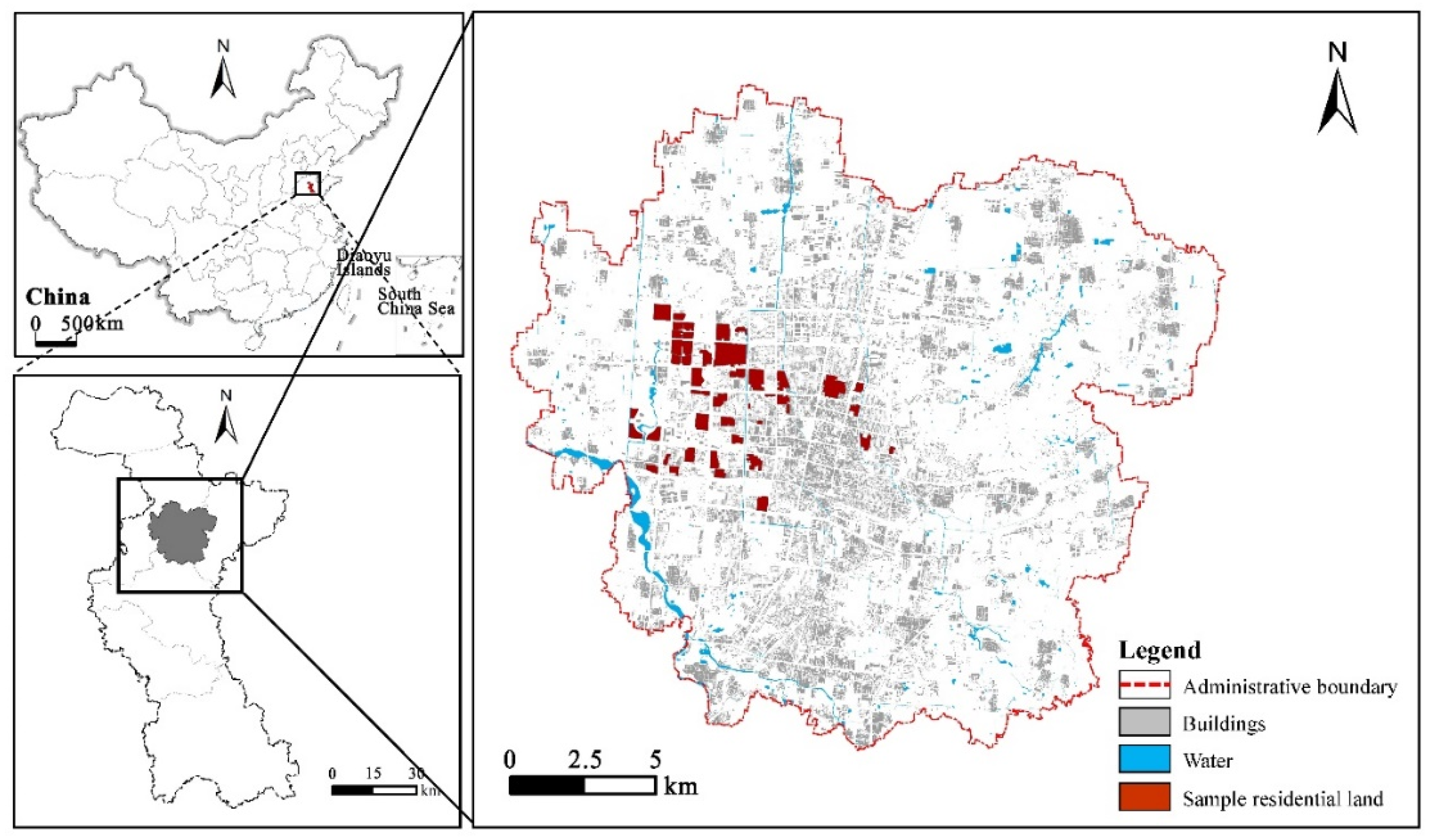
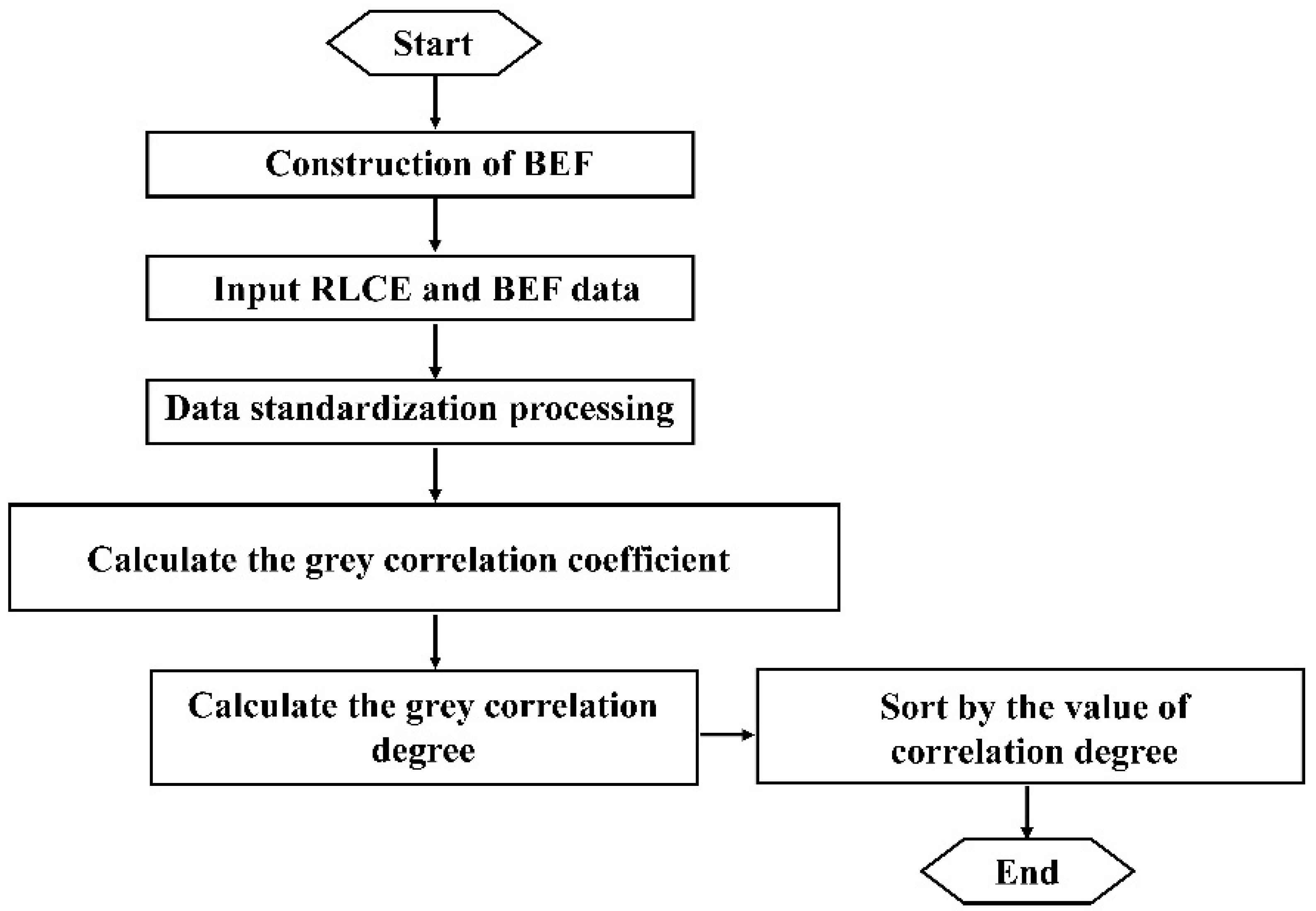
In the representative resource-based city of Zibo, China, 45 residential lands are selected as research objects. The Grey correlation analysis method and Universal global optimization method are proposed to explore the effects of BEF on RLCE using advanced metering infrastructure (AMI) data provided by the Zibo power supply company. The study starts by emphasizing the significance of the effects of BEF on RLCE. The Section 2 elaborates on prior research and the knowledge gaps in the literature. The Section 3 explains the study area, research data, and methods. In the Section 4, the study presents the results of this study in three subsections: RLCE and BEF, Correlations between BEF and RLCE, and Regression of BEF and RLCE. The Section 5 further discusses the effects of intensity, density, morphology, and land on RLCE, as well as the perspective of urban planning strategies to reduce RLCE and the detailed applications of the results. The Section 6 presents the conclusions.

3. Materials and Methods

3.1. Study Area

Zibo (35° 55′–37°17′ N, 117°32′–118°31′ E) is located in the east of China. Taking Zibo as the study area is mainly based on the following considerations:
  • Zibo has typical climate characteristics of a hot summer and cold winter, and its urban planning can better reflect the sensitivity and adaptability to climate change. In addition, to ensure the comfort of living, it is necessary to use air conditioning to cool down in summer, and the RLCE is generally high.
  • The urbanization of Zibo is high. In 2020, the permanent resident population of Zibo was 4,704,100, and the urbanization rate was 74.27%. The urbanization rate is higher than the average level of Shandong, lower than Qingdao, and ranking second in Shandong Province.
  • The development of Zibo is still rapid and more and more residential lands will be continuously developed and constructed, requiring that the heavy carbon emissions reduction task be faced. This study can provide a basis for the low-carbon design of residential lands in Zibo in the future.
  • The old and new urban areas of Zibo have typical characteristics of dual urban structure, which are manifested by rich living forms and diverse residential land types, making the selection of samples more representative.
  • Zibo is a typical resource-based city with high carbon emissions, which can provide a reference for the low-carbon development of other resource-based cities.
To ensure the diversity of BEF and the available building energy consumption data, the built-up area in Zhangdian District, the main urban area of Zibo City, was selected as the study area. According to the aim of the study on the effects of BEF on RLCE, the selection of residential land samples should control the other variables affecting RLCE as much as possible under the premise of ensuring the diversity of BEF. In the selection of residential lands samples, the study needs to cover as many types of residential land as possible and follows the principles that the residential land area are different and greater than 1 hm2, the boundaries are clearly defined, the buildings are composed of a uniform type, the housing types are consistent, the population is greater than 1000, the lands surrounding the residential lands have been completed, there are rich land use types within 500 m, the delivery time is more than 3 years, and the occupancy rate is higher than 50%, etc. Moreover, the residential land samples should cover different locations and construction times. Combined with Google images and a questionnaire survey, 45 residential land samples were selected. The study area and distribution of residential land samples are shown in Figure 1.

3.2. Research Data

The research data involved in this study included building energy consumption data and BEF data in 2021, as presented in Table 1. Among them, the building energy consumption data included the residential land’s name, location, and electricity consumption, which are provided by the Zibo power supply company. The BEF data included buildings, lands, populations, green area, and the ratio of various types of land within 500 m around the residential lands, which are provided by various government departments of Zibo (Table 1).

3.3. Methods

3.3.1. RLCE Measurement Method

The energy consumption of residential land mainly includes buildings, transportation, waste treatment, etc. Among them, building energy consumption accounts for the largest proportion [32]. The actual energy consumption of buildings includes central heating, electricity, and gas, which is mainly used for heating, cooling, lighting, equipment, etc. The heating methods are different in different climates in China. For example, central heating is mainly used in severe cold and cold areas, while electricity is mainly used in hot summer and cold winter, hot summer and warm winter, and mild climate areas. In this study, we only concentrate on electricity consumption. On the one hand, electricity consumption is an important source of RLCE, but, on the other hand, it is most closely related to the BEF. Some studies have also confirmed this. Zhang et al. collected RLCE in Changxing, Zhejiang Province, China, and found that electricity consumption carbon emissions are the main source of emissions, accounting for more than 98%, while natural gas consumption carbon emissions account for only about 1% [33]. Therefore, the RLCE is mainly characterized by electricity consumption carbon emissions in this study. According to the carbon emissions coefficient, the RLCE is calculated according to Equation (1) by using the electricity consumption of each residential land [34]. The measurement method of RLCE is defined as follows:
E = AD × EF
where E is carbon emissions (kg), AD is electricity consumption, and EF is the carbon emissions coefficient. Among them, AD is the annual electricity consumption of residential land provided by the Zibo power supply company. EF uses the average carbon emissions per unit of electricity consumption in North China and the value is 1.246 kgCO2/kW h. Additionally, residential land carbon emissions intensity (RLCEI) is the ratio of RLCE to the residential land area [35], and the measurement method of RLCEI is defined as Equation (2):
I = E/S
where I is carbon emissions intensity (kg/m2), E is carbon emissions (kg), and S is the area of residential land (m2).

3.3.2. BEF Measurement Methods

According to the national residential land planning and control standards, combined with relevant literature research, expert interviews, and comparative analysis of multiple field investigations of different residential lands, BEF are mainly divided into four categories in this study: intensity, density, morphology, and land, with a total of 16 BEF. Among them, the intensity includes building area (BA), land area (LA), floor area ratio (FAR), and greening rate (GR). The FAR is the ratio of the total floor area of residential land to the land area, reflecting the intensity and efficiency of land use, as well as the difference in the land price. The GR is the ratio between the sum of all kinds of green land area and the residential land area, reflecting the green level of residential land.
The density includes building density (BD) and population density (PD). The morphology includes the height of building height (BH), building shape coefficient (BSC), and high-rise buildings ratio (HRBR). The BSC is an architectural design term, which refers to the ratio of the external area of the building in contact with the outdoor atmosphere to the volume enclosed. Buildings with small volumes and complex shapes, as well as bungalows and low-rise buildings, have large shape coefficients that are unfavorable for energy saving. Buildings with large volumes and simple shapes, as well as multi-story and high-rise buildings, have small shape coefficients that are more beneficial to energy saving. The HRBR is the ratio of the total building area of high-rise residential buildings to the total building area of residential land, which is closely related to BD, GR, and BH. It is also an important factor affecting the RLCE.
The land includes land construction time (LCT), commercial land ratio within 500 m (CLR), industrial land ratio within 500 m (ILR), green land ratio within 500 m (GLR), cultural and sports land ratio within 500 m (CSLR), administrative land ratio within 500 m (ALR), and transportation land ratio within 500 m (TLR). Among them, the CLR is the ratio of the area of commercial land within 500 m from the boundary of residential land to all the land within 500 m, which can reflect the surrounding environmental characteristics of residential land to a certain extent.
The measurement methods of different types of BEF are shown in Table 2.

3.3.3. Grey Correlation Analysis Method

Grey theory is a system science theory put forward by Deng Julong for the first time in 1982 [48]. The Grey correlation analysis method is a system theory for the statistical analysis of uncertain systems with little data and poor information [49,50]. It is one of the important achievements in the field of uncertainty system research.
Compared with the Pearson correlation coefficient, which can only reflect the linear correlation between variables, Rank correlation is more suitable for stratified variables. The Grey correlation analysis method represents the most generalized correlation. No matter whether the two variables are nonlinear function correlations or hyperfunction correlations, this correlation can be detected and a high grey correlation value is given [51]. Therefore, relevant studies are gradually increasing [52,53]. For example, Liu et al. analyzed the temporal and spatial evolution characteristics of carbon emissions in China’s Yangtze River Delta and its relationship with economic development and ecology based on the Grey correlation analysis method and then put forward optimization suggestions [52]. Its basic idea is the geometric similarity of the time series of the two variables. The more similar the shape, the higher the correlation between the two variables. The dominant factors are determined by calculating the correlation degree between multiple factors and the same reference sequence. In this paper, the RLCE is defined as the dependent variable (y) and BEF as the independent variable (x), and the Grey correlation coefficients are calculated in Python 3.8. According to the method proposed by Wu et al. [53], they are defined as Equations (3)–(6):
C t = 1 m × l i = 1 m j l ϵ j t
where C t is the correlation degree between BEF and RLCE, m is the number of BEF, l is the number of RLCE. ϵ j t is the Grey correlation coefficient, and the data standardization method can be used to improve accuracy [8]. The Grey correlation coefficient is estimated using Equation (4):
ϵ j t = m i n i   m i n j Z i X t Z j Y t + ρ   m a x i   m a x j Z i X t Z j Y t Z i X t Z j Y t + ρ   m a x i   m a x j Z i X t Z j Y t
where Z i X t is the standard value of BEF, Z j Y t is the standard value of RLCE, and ρ is the resolution coefficient, which is 0.5. According to the method proposed by Olu-Ajayi et al. [8], the range standardization method can be used to obtain Z i X t and Z j Y t and it is defined as Equation (5):
Z i j = X i j m i n i   X i j m a x i   X i j m i n i   X i j
The Grey correlation degree of BEF and RLCE can be obtained by taking the mean value of ϵ j t according to time and the residential land samples, respectively [53], and it is defined as Equation (6):
γ i j = 1 k i = 1 k ϵ j t
where k is the number of samples, γ is the Grey correlation coefficient of BEF and RLCE, and the larger the value of γ , the stronger the correlation. The classification of Grey correlation is as follows: 0.8–1 indicates a very strong correlation, 0.6–0.8 indicates a strong correlation, 0.3–0.6 indicates a general correlation, and 0–0.3 indicates a weak correlation [54]. In this study, the Grey correlation coefficients are calculated in Python 3.8, the flowchart of the Python code is shown in Figure 2.

3.3.4. Universal Global Optimization Method

When there is a nonlinear relationship between dependent variables and independent variables, the function formula is often complex in nonlinear function fitting. Therefore, global convergence and local convergence must be fully considered in function fitting calculations [55,56]. 1stOpt is a comprehensive tool package for mathematical optimization analyses that was independently developed by 7d soft High Technology Inc. The core of its calculation is the fitting calculation based on the Universal global optimization method to find the optimal fitting function. The method supports more than 5000 functions and has been widely verified in relevant studies [57,58]. For example, Liu et al. analyzed the relationship between carbon emissions and population, cultivated land area, and vehicle ownership in Beijing and the surrounding five North China provinces through the Universal global optimization method based on 1stOpt and verified the feasibility of the method [56]. Therefore, based on 1stOpt software, the Universal global optimization method is selected to further quantitatively analyze the relative importance of BEF on RLCE and then calculate its determination coefficient, R2. Generally, the closer the R2 value is to 1, the higher the fitting degree between the variables. If the value of R2 is above 0.6, it is considered that the fitting degree of the regression equation is excellent, and if it is less than 0.3, it is considered that the fitting degree of the regression equation is poor [57].

4. Results

4.1. RLCE and BEF

The measurement is run in Arcgis10.2 and the measurement results of residential land carbon emissions (RLCE) and residential land carbon emissions intensity (RLCEI) are shown in Figure 3. As expected, in terms of RLCE, the average value of RLCE is 6,814,879.58 kgCO2. The highest RLCE is Century Garden (No.35) with carbon emissions of 27,954,195.74 kgCO2. It is located at the junction of the old urban area and the new urban area of Zhangdian District and was completed and put into use in 2007. Therefore, the occupancy rate is relatively high and it is also the residential land with the largest LA in all samples. Meanwhile, the lowest RLCE is Hengxing Garden (No.22) with carbon emissions of 168,763.22 kgCO2. It is located in the south of No.35 and was completed and put into use in 2012. In terms of RLCEI, the average value of RLCEI is 63.60 kgCO2/m2. The largest RLCEI is Prospective Garden (No.40) with a carbon emissions intensity of 168.52 kgCO2/m2. It is also located at the junction of the old urban area and the new urban area of Zhangdian District, on the north side of No.35, which includes several villas with 1–3 floors. Meanwhile, Jinshilvcheng (No.22) has the smallest RLCEI and is located in the new area of Zhangdian District. It is mainly composed of 28 floors of residential buildings and the carbon emissions intensity of No. 22 is 1.05 kgCO2/m2.
Using scatter plot analysis, it can be seen that a higher BA is often accompanied by higher LA and BSC, and a higher BH is often accompanied by lower BSC and higher FAR (Figure 4). With BA ranging from 30,800 m2 to 1,125,422 m2, LA increases from 18,501 m2 to 796,499 m2 and BSC increases from 0.50 to 5.2. With BH ranging from 5 m to 32 m, BSC decreases from 5.19 to 0.60 and FAR increases from 1 to 2.80. Additionally, LCT also correlates with BH, FAR, BSC, and HRBR.

4.2. Correlations between BEF and RLCE

Based on the collection of measurement data of BEF, this study analyzes the correlation between BEF and RLCE and obtains the correlation coefficient between BEF and RLCE (Figure 5). The results show that all the selected BEF have a strong correlation with RLCE. Among them, the correlation coefficients between BA, BSC, GA, LA, FAR, BD, and RLCE are more than 0.9600, which is 0.9713, 0.9672, 0.9663, 0.9645, 0.9621, and 0.9611, respectively. The correlation coefficients between CLR, LCT, BH, PD, CSLR, GLR, TLR, HRBR, ALR, and RLCE are more than 0.9200, which is 0.9523, 0.9520, 0.9500, 0.9491, 0.9410, 0.9355, 0.9301, 0.9290, and 0.9220, respectively. The correlation coefficient between ILR and RLCE is 0.9175. Therefore, each BEF is related to RLCE in varying degrees, but the importance of each BEF still needs to be further analyzed by using the Universal global optimization method.

4.3. Regression of BEF and RLCE

In this study, the Universal global optimization method is used to fit the optimal functional relationship equation between BEF and RLCE and the R2 is calculated. The closer the R2 value is to 1, the higher the fitting degree between BEF and RLCE. The Universal global optimization method simulation is run in 1stOpt1.5. The fitting parameters and results are shown in Table 3 and Figure 6, which can clearly show the fitting accuracy of BEF and RLCE.
Among BEF, the R2 of BSC, HRBR, BH, PD, and ILR are above 0.6 and are the key BEF. The R2 of LA, BA, FAR, and GLR are above 0.4 and are the secondary influencing BEF. The R2 of LCT is 0.075, which shows that it has the least effect on RLCE. Among different categories, the R2 of LA is 0.557, which is higher than BA and FAR, and is the main intensity factor affecting RLCE. The R2 of PD is 0.679, which is higher than that of BD—the main density factor affecting RLCE. The R2 of BSC is 0.754, which is higher than BH and HRBR and is the main morphology factor affecting RLCE. The R2 of ILR is 0.634, which is higher than LCT, CLR, CSLR, TLR, ALR, and GLR, and is the main land factor affecting RLCE (Table 4). These results can clarify the order in which the BEF affects the RLCE, distinguish the importance of different groups of BEF for reducing the RLCE, and improve the pertinence of low-carbon urban planning strategies.
To further analyze the effects of key BEF on RLCE, the relationship between BSC, HRBR, BH, PD, ILR, and RLCE are further visualized. The results show that there is a complex nonlinear functional relationship between BSC, HRBR, BH, PD, ILR, and RLCE. Among them, BSC, BH, PD, and ILR have positive effects on RLCE, while HRBR and RLCE decreased first and then increased (Figure 7).

4.4. Comparison with Existing Methods

To further compare the reliability of the methods, a Pearson correlation coefficient and multiple linear regression were used to conduct comparative tests. Detailed information on the Pearson correlation coefficient is shown in Table 5. The results show that the BEF correlation coefficients in the Pearson correlation are smaller than that in the Grey correlation analysis, and the values of some BEF are not significant, with the sig value greater than 0.05—such as FAR, GA, BD, etc. This means that the Pearson correlation coefficient has difficulty capturing the relationship between BEF and RLCE.
As shown in Table 6, the advantages of the Universal global optimization method are revealed by comparing the regression results of different methods. In the process of multiple linear regression analysis, the R2 of the method was only 0.376, which is lower than the 0.606 of the Universal global optimization method. The comparison results illustrated that the proposed method was highly reliable.

5. Discussion

The Data statistical analysis results demonstrate that different kinds of BEF lead to distinctively different carbon emissions for residential lands in Zibo. However, the mechanism of BEF that affects RLCE according to the quantitative results needs to be explored to provide effective and scientific planning suggestions at the urban design level.

5.1. Effects of Intensity

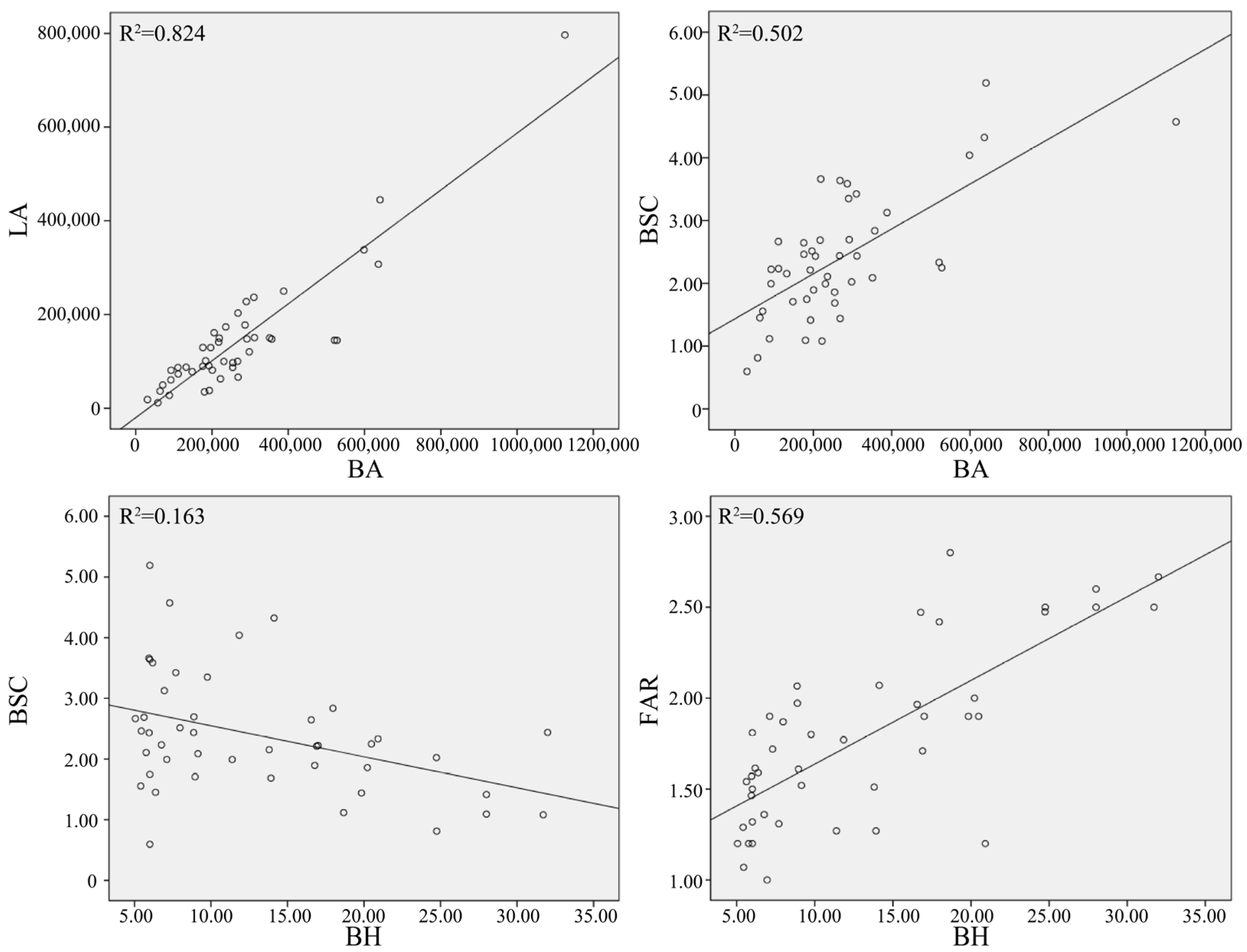
BA, LA, FAR, and GR are the four main factors to describe the intensity. Among them, the R2 of LA is 0.557, which is higher than the R2 of BA, FAR, and GR. Therefore, LA is the primary intensity factor affecting RLCE and is positively correlated with RLCE. The reason for this is due to the increase of LA, which leads to the BA of residential lands also increasing accordingly. As a symbol of urban spatial intensity, BA is usually proportional to it. Generally, residential land with a higher carbon emission combines with a larger LA, higher BA, taller FAR, and lower GR. Additionally, a lower carbon emission residential land is characterized as lower LA with sparse BA, smaller FAR, and larger GR. Although higher BA is an important indicator to measure the economy of land use, it also means higher energy consumption and carbon emissions demand and causes more users, electrical equipment, and lighting to release more heat in a building. Additionally, the high BA also has an impact on the daylighting, thermal radiation, and airflow of the land. High BA can increase the building surface area of the land to absorb solar radiation, thus affecting the microclimate of the land. It can be argued that high BA residential lands alter their thermal environment in the form of raising the ambient temperature relative to that of low BA residential lands, thereby indirectly increasing the energy consumption and carbon emissions. Some studies have also proved this. For example, Garbasevschi et al. found that the RLCE with larger LA in the United States is much higher than those with smaller LA [25]. Zhang et al. conducted an empirical study on the relationship between RLCE and LA in Nanjing, China by using the ENVI-met simulation data. The results show that in the suburbs with larger LA, the RLCE is higher, while in the central urban areas with smaller LA, the RLCE is lower [59]. A high GR means there is more green space or open space in the residential land. The green space dominated by deciduous trees has greatly weakened wind resistance in winter, which is equivalent to a square of open space. In addition, the open space as an open and well-connected wind passage provides more heat loss efficiency for buildings through a higher ventilation rate. It is evident from previous studies that a location with a lower green space ratio is warmer compared to a district with a higher GSR in winter [12]. Therefore, the conclusions also further verify the applicability of the existing research conclusions to the type of resource-based cities.
Additionally, the indicators to measure LA include block scale and road network density. In a certain area, the higher the road network density and the smaller the block scale mean the smaller the LA. Small scale lands can provide a variety of travel options, which can increase pedestrian accessibility and reduce traffic energy consumption carbon emissions.

5.2. Effects of Density

BD and PD are two main factors to describe density. Among them, the R2 of PD is 0.679, which is higher than the R2 of BD. Therefore, PD is the primary density factor affecting RLCE and is positively correlated with RLCE. PD mainly reflects the number of people on the unit land. The effects of PD on RLCE are mainly reflected in the types of energy consumption for different types of buildings, such as lighting, heating, and refrigeration in residential buildings, as well as the energy consumption of lighting, heating, refrigeration, and office equipment in public buildings. The effects occur because there is much more anthropogenic heat generated from heating buildings and other daily human activities in high PD residential lands. When the PD is high, it means that the use intensity of buildings is high and the carbon emissions are correspondingly high. Therefore, it is feasible to reduce RLCE by increasing PD when preparing for low-carbon urban planning.
As an important BEF, PD has a close relationship with other BEF. Based on the definition of PD, Timmons, et al. theoretically deduced the relationship between FAR, LA, and BA [42]. That is, PD is the product of the proportion of residential land, population per unit building area, and FAR of residential land. In addition, it has been further proved that the increase of PD can promote the increase of urban heat island intensity and the expansion of its scope, and further affect the RLCE [60]. In general, PD is positively correlated with BA and urban heat islands but negatively correlated with housing areas. The higher the PD, the greater the BA and heat island effect, the smaller the housing area, and, therefore, the RLCE increases significantly.

5.3. Effects of Morphology

The effect of morphology on RLCE is greater than that of intensity, density, and land. The results show that the R2 of BSC, HRBR, and BH are significantly higher than that of other BEF, especially intensity, which is different from other studies. The study holds that in resource-based cities such as Zibo, the intensity of residential lands is homogeneous to a certain extent and the difference in RLCE is more reflected in the difference in morphology. Therefore, compared with the optimization of BEF, which focuses on intensity in big cities, the optimization of BEF should pay more attention to morphology in the reduction of RLCE in resource-based cities.
Among morphology, BSC and BH are positively correlated with RLCE. BSC refers to the ratio of building surface area to volume. Under the same conditions, the larger the BSC, the larger the surface area of heat exchange between the unit volume building and the atmosphere, and the more heat gain or heat dissipation per unit volume through the unit surface area. On the contrary, the smaller the BSC, the less heat gain or heat dissipation per unit volume through the unit surface area, which is an important aspect affecting RLCE.
BH can change the microclimate environment around the residential lands by affecting the sunshine conditions, temperature, and wind environment. The microclimate environment is an important factor affecting building energy consumption, such as building heating and cooling, which significantly increases RLCE. Some studies have also proved this. For example, Zoulia et al. compared the air temperature data of 30 meteorological stations in Athens and found that the urban heat island caused the temperature in the urban area to rise by 10 °C. Accordingly, the energy consumption of urban buildings in summer doubled that in the suburbs [61]. Waldron et al. used virvil plugin software to conduct a simulation analysis and perform comparative research on the effects of BH on building energy consumption. The results show that the energy consumption per unit building area of high-rise, middle-rise, and low-rise buildings increases in turn, but the total building energy consumption and carbon emissions decrease in turn [62]. The reason is that the increase in BH will lead to a corresponding increase in BA and PD, and then an increase in RLCE. Additionally, BH can also affect building energy consumption in two other ways. (1) By affecting the change of air temperature, the building energy consumption in the process of heat and moisture transfer is affected. (2) By affecting the indoor and outdoor air exchange of the building, which causes the heat balance of the house to be affected. HRBR and RLCE show a changing relationship of first decreasing and then increasing.

5.4. Effects of Land

The impact of land on RLCE in resource-based cities such as Zibo is less than that in big cities. In some studies, the land is an important BEF affecting RLCE. However, in our study, except for the high R2 of ILR, the R2 of LCT, CLR, CSLR, TLR, ALR, and GLR are 0.075, 0.383, 0.371, 0.324, 0.399, and 0.416. The results show that, in terms of reducing RLCE, the carbon reduction benefit of land optimization within 500 m around residential lands in resource-based cities is less than that of the other three types of BEF. Zibo is a representative resource-based city, with a high ILR and scattered distribution, which makes this factor special. As is shown in Figure 4, ILR is positively correlated with RLCE, which means that in residential lands with high ILR, RLCE is high. The reason for this is that the more industrial land around residential lands, the more employment opportunities. Therefore, more residents choose to work nearby and spend more time at home. Although the choice of low-carbon commuter transportation can be increased, it will also increase the carbon emissions of residents’ electricity consumption to a certain extent.

5.5. Applications

In recent years, how to accurately analyze the effects of BEF on RLCE has been a great concern [63]. The results obtained in this study can be used to supplement and improve the control index system of the existing urban planning at the medium and micro scales. This is of great significance for guiding policymakers to formulate targeted emission reduction policies or helping urban planners to formulate low-carbon urban planning schemes that are more targeted to control RLCE. The detailed applications are shown in the following two aspects.
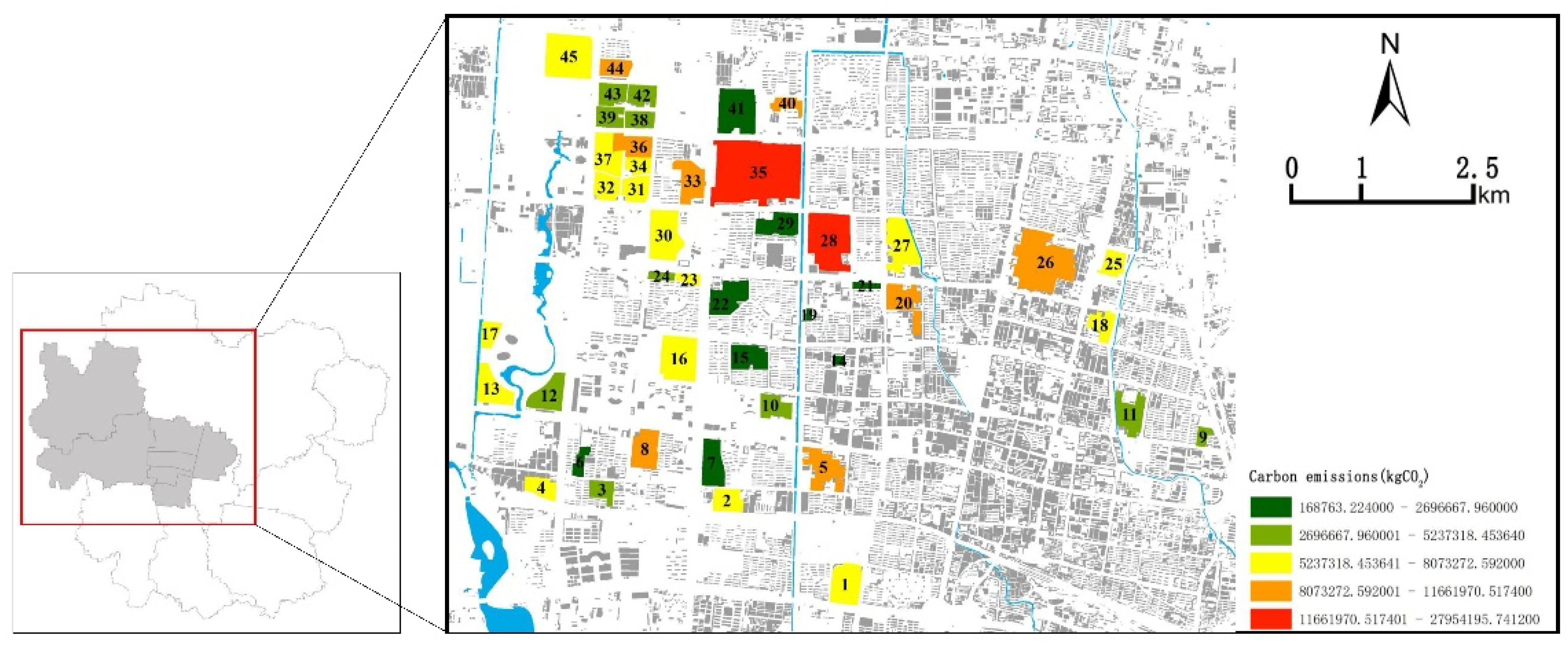
For one thing, the measurement methods of RLCE and BEF were proposed in this study and a database was established to provide the carbon emissions of each residential land with a clear geographical location and boundary, which can identify the key carbon reduction regions and provide more accurate information for the local government’s carbon emission control and management (Figure 8). This is also very essential for low-carbon urban planning as the database also provides sufficient data for our further study of the relationship between RLCE and the BEF and allows for the visualization of how and why existing residential lands affect carbon emissions due to their intensity, density, morphology, and land, which can be additional support for urban planning to achieve carbon reduction.
Another thing is to further illustrate the applicability of the analysis results, which can be used to reduce the carbon emissions of the urban planning schemes. According to the results of RLCE and BEF in Section 4.2 and 
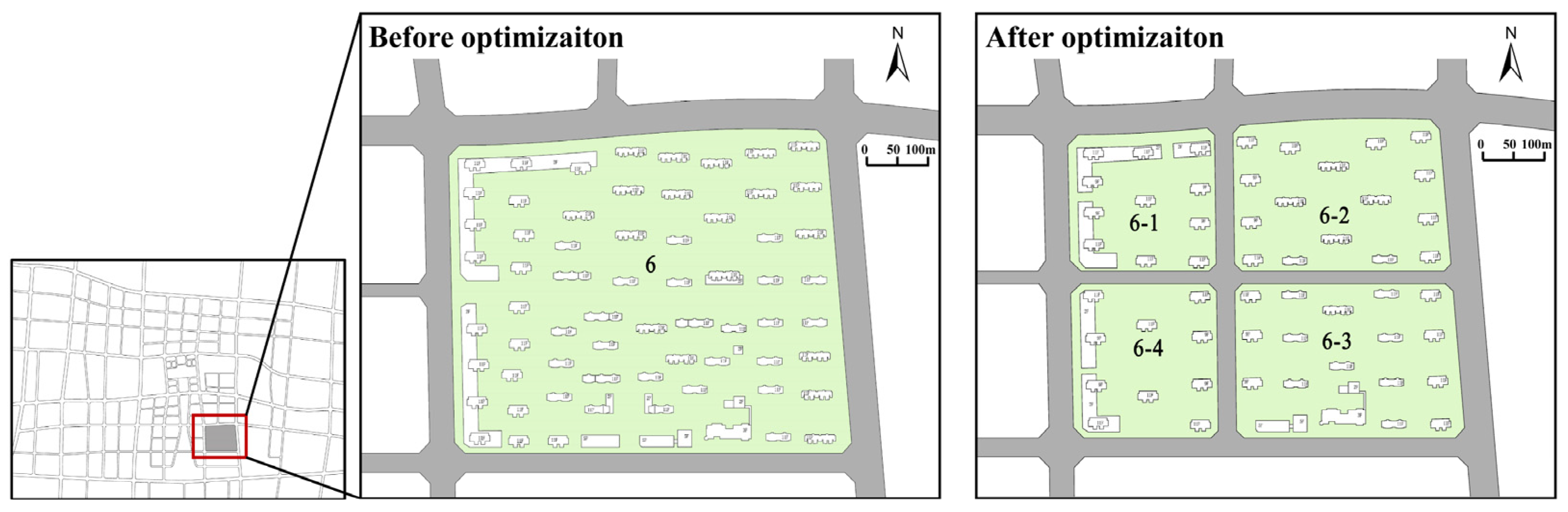
Section 4.3, the specific low-carbon optimization methods for the BEF on RLCE in the urban planning scheme can further be proposed. Then, by predicting the urban planning scheme after optimization again—and comparing it with the carbon emissions prediction results of the urban planning scheme before optimization—the carbon reduction benefits of low-carbon optimization of urban planning schemes on RLCE can be evaluated. Taking residential land 6 in the urban planning scheme as an example to illustrate in detail (Figure 9), the carbon emissions of residential land 6 before optimization was 1.1660 × 10⁴ tCO2 and the carbon emissions of residential lands 6-1, 6-2, 6-3, and 6-4 after optimization were 8.8700 × 10³ tCO2, which was a reduction of 2.7900 × 10³ tCO2 and accounted for 23.93% of the carbon emissions of residential land 6 before optimization.

5.6. Limitations and Further Improvements

There are also some uncertainties in this study. Firstly, although the research methods we proposed provide a new possibility to explore the effects of BEF on RLCE under the condition of limited statistical samples, there are only 45 residential land samples, which will affect the accuracy of the results. Secondly, compared with other studies, the RLCE is represented by electricity consumption carbon emissions in this study, without considering the gas, transportation, and waste transfer. Although it is feasible, it will also have errors. Thirdly, the time series of building energy consumption data needs to be extended. The robustness of the results of this study can be improved by analyzing changes in panel data over many years. Finally, the optimal BEF could be further studied to reduce the RLCE.

6. Conclusions

In this study, we quantitatively investigated the effects of BEF on RLCE using advanced metering infrastructure (AMI) data in Zibo, a representative resource-based city in China. Forty-five residential lands and the corresponding building energy consumption data, as well as 16 BEF surrounding these residential lands, were studied in detail through a combination approach of the Grey correlation analysis method and the Universal global optimization method. Some conclusions can be obtained as follows.
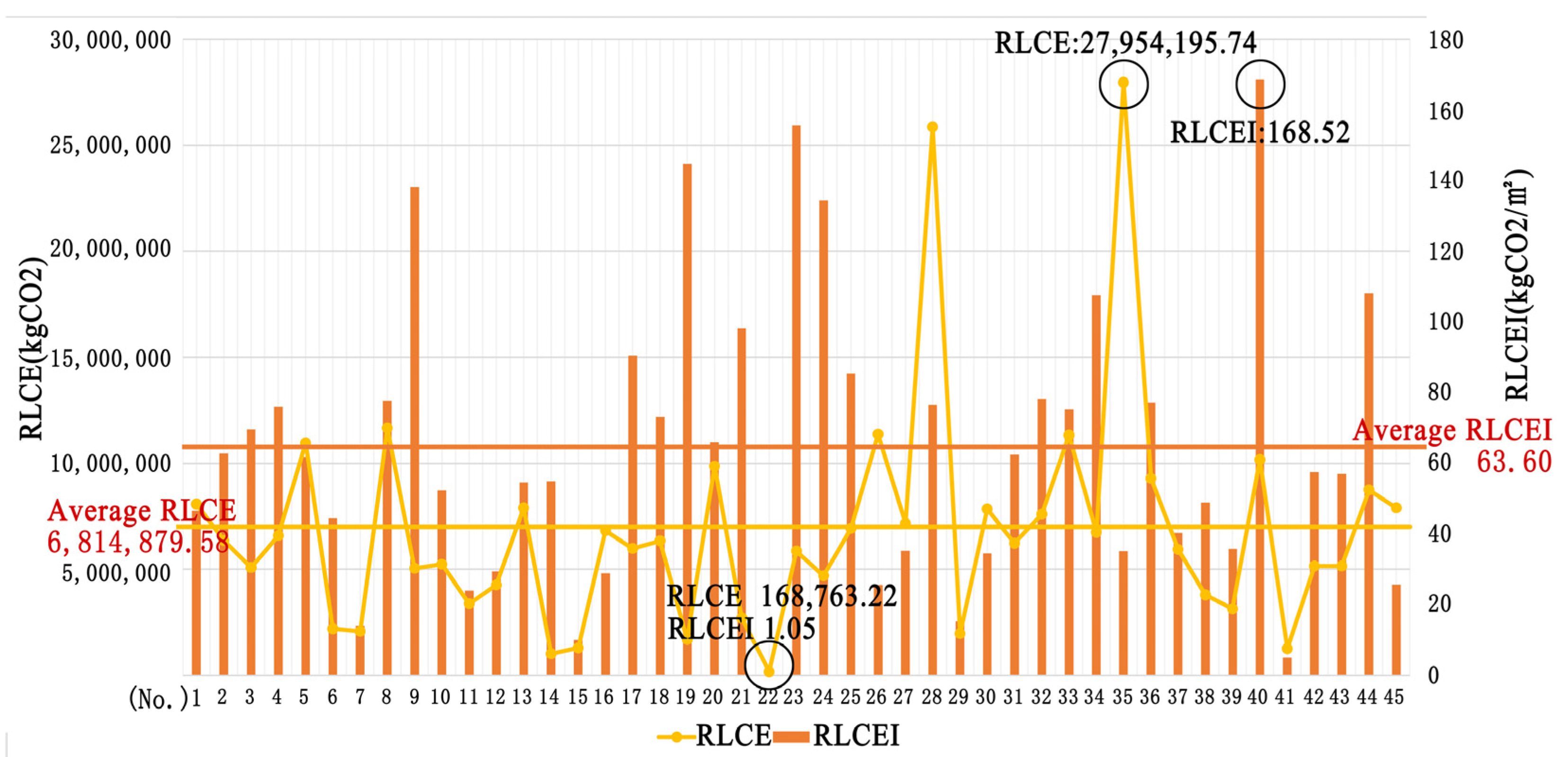
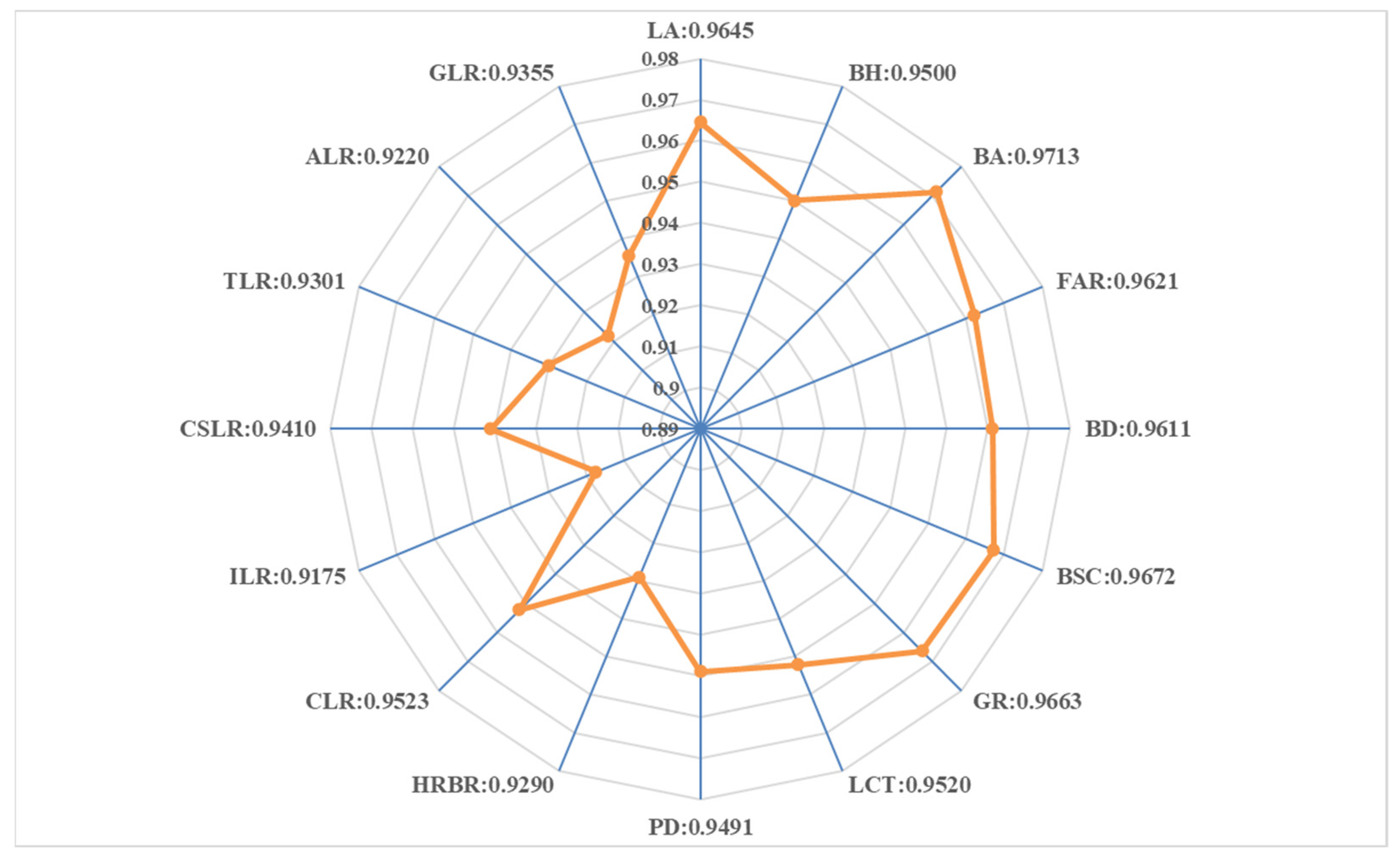
BEF have remarkable effects on RLCE. Among them, the correlation coefficients between BA, BSC, GA, LA, FAR, BD, and RLCE are 0.9713, 0.9672, 0.9663, 0.9645, 0.9621, and 0.9611; the correlation coefficients between CLR, LCT, BH, PD, CSLR, GLR, TLR, HRBR, ALR, and RLCE are 0.9523, 0.9520, 0.9500, 0.9491, 0.9410, 0.9355, 0.9301, 0.9290, and 0.9220; and the correlation coefficient between ILR and RLCE is 0.9175.
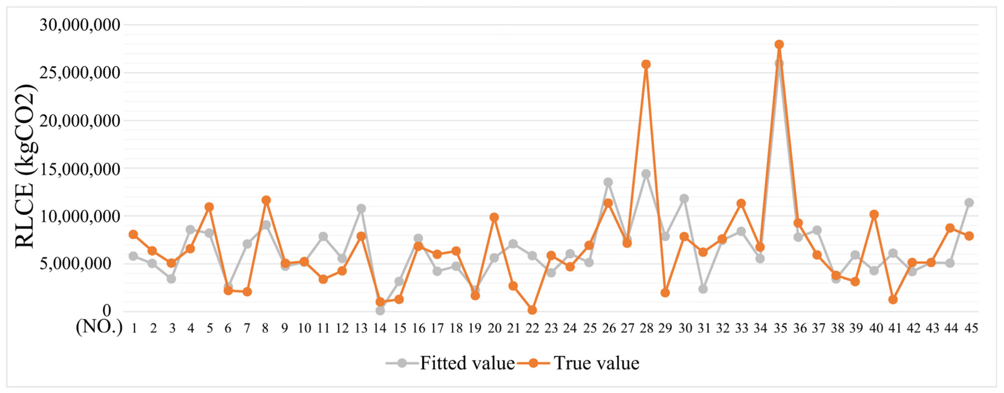
BEF are satisfactorily and nonlinearly related to RLCE, and the value of correlation coefficient R is 0.788, while R2 is 0.606. Among BEF, the R2 of BSC, HRBR, BH, PD, and ILR are 0.754, 0.699, 0.684, 0.679, and 0.634, and are the key BEF. The R2 of LA, BA, FAR, and GLR are 0.557, 0.548, 0.429, and 0.416, and are the secondary influencing BEF. The R2 of LCT is 0.075 and has the least effect on RLCE.
LA is the primary intensity factor affecting RLCE and is positively correlated with RLCE. PD is the primary density factor affecting RLCE and is positively correlated with RLCE. The effects of morphology on RLCE are greater than that of intensity, density, and land. Among morphology, BSC and BH are positively correlated with RLCE, while HRBR and RLCE show a changed relationship of first decreasing and then increasing. The effects of land on RLCE in resource-based cities such as Zibo are less than that in big cities.
For this study, after obtaining the analysis results above, the possible urban planning strategies in residential land can be proposed for carbon emissions reduction. By optimizing the density, function, form, and land, such as reducing LA, PD, BSC, BH, and increasing HRBR within a certain range, urban planning can ultimately achieve the effects of carbon emissions reduction. The results obtained in this study can be used to supplement and improve the control index system of the existing urban planning at the medium and micro scales, which can provide valuable guidance for emission reduction policies and low-carbon planning. Moreover, the results provide a basis for establishing the prediction method of RLCE and putting forward suggestions for the low-carbon optimization of BEF and can be used to predict and reduce the carbon emissions of urban planning schemes. Overall, it was discussed that the onus is on a group of people, including designers, urban planners, policymakers, and building managers, to take measures to put forward energy-saving-oriented urban planning strategies and ensure their implementation, which is of great significance to mitigate climate change and develop low-carbon cities.

Author Contributions

Conceptualization, Q.L., X.Z., H.Z., Y.L. (Yili Liao) and P.L.; data curation, Q.L., H.Z., Y.L. (Yichen Liao) and X.Z.; formal analysis, Q.L., P.L., Y.L. (Yili Liao) and P.L.; funding acquisition, Q.L. and X.Z.; investigation, Q.L., Y.L. (Yichen Liao) and Y.L. (Yili Liao); methodology, X.Z., Y.L. (Yili Liao) and H.Z.; project administration, P.L., Y.L. (Yichen Liao) and H.Z.; resources, Y.L. (Yili Liao) and Y.L. (Yichen Liao); software, X.Z. and Q.L.; supervision, P.L. and Y.L. (Yili Liao); validation, X.Z.; visualization, Q.L. and Y.L. (Yichen Liao); writing—original draft, Q.L. and Y.L. (Yichen Liao); writing—review & editing, X.Z. and P.L. All authors have read and agreed to the published version of the manuscript.

Funding

This research was funded by the National Natural Science Foundation of China, grant no. 51878393; the Youth fund of Shandong Natural Science Foundation, grant no. ZR202108090061.

Institutional Review Board Statement

Not applicable.

Informed Consent Statement

Not applicable.

Data Availability Statement

All data underlying the results are available as part of the article, and no additional source data are required.

Conflicts of Interest

The authors declare no conflict of interest.

Abbreviations

ALRAdministrative Land Ratio Within 500 m
AMIAdvanced Metering Infrastructure
BABuilding Area
BDBuilding Density
BEFBuilt Environment Factors
BHBuilding Height
BSCBuilding Shape Coefficient
CLRCommercial Land Ratio Within 500 m
CSLRCultural and Sports Land Ratio Within 500 m
FARFloor Area Ratio
GLRGreen Land Ratio Within 500 m
GRGreening Rate
HRBRHigh-Rise Buildings Ratio
ILRIndustrial Land Ratio Within 500 m
LALand Area
LCTLand Construction Time
PDPopulation Density
RLCEResidential Land Carbon Emissions
RLCEIResidential Land Carbon Emissions Intensity
TLRTransportation Land Ratio Within 500 m
UCLUrban Construction Land

References

  1. Yang, J.; Zhan, Y.; Xiao, X.; Xia, J.C.; Sun, W.; Li, X. Investigating the diversity of land surface temperature characteristics in different scale cities based on local climate zones. Urban Clim. 2020, 34, 100700. [Google Scholar] [CrossRef]
  2. Zhang, Y.; Liu, Y.; Wang, Y.; Liu, D.; Xia, C.; Wang, Z.; Wang, H.; Liu, Y. Urban expansion simulation towards low-carbon development: A case study of Wuhan, China. Sustain. Cities Soc. 2020, 63, 102455. [Google Scholar] [CrossRef]
  3. Liu, L.C.; Wu, G.; Wang, J.N.; Wei, Y.M. China’s carbon emissions from urban and rural households during 1992–2007. J. Clean. Prod. 2011, 19, 1754–1762. [Google Scholar] [CrossRef]
  4. He, B.J.; Zhao, D.; Dong, X.; Xiong, K.; Feng, C.; Qi, Q.; Darko, A.; Sharifi, A.; Pathak, M. Perception, physiological and psychological impacts, adaptive awareness and knowledge, and climate justice under urban heat: A study in extremely hot-humid Chongqing, China. Sustain. Cities Soc. 2022, 79, 103685. [Google Scholar] [CrossRef]
  5. Yang, J.; Wang, Y.; Xue, B.; Li, Y.; Xiao, X.; Xia, J.; He, B. Contribution of urban ventilation to the thermal environment and urban energy demand: Different climate background perspectives. Sci. Total Environ. 2021, 795, 148791. [Google Scholar] [CrossRef]
  6. Yang, J.; Jin, S.; Xiao, X.; Jin, C.; Xia, J.; Li, X.; Wang, S. Local climate zone ventilation and urban land surface temperatures: Towards a performance-based and wind-sensitive planning proposal in megacities. Sustain. Cities Soc. 2019, 47, 101487. [Google Scholar] [CrossRef]
  7. He, B.J. Potentials of meteorological characteristics and synoptic conditions to mitigate urban heat island effects. Urban Clim. 2018, 24, 26–33. [Google Scholar] [CrossRef]
  8. Olu-Ajayi, R.; Alaka, H.; Sulaimon, I.; Sunmola, F.; Ajayi, S. Building energy consumption prediction for residential buildings using deep learning and other machine learning techniques. J. Build. Eng. 2022, 45, 103406. [Google Scholar] [CrossRef]
  9. He, B.J. Towards the next generation of green building for urban heat island mitigation: Zero UHI impact building. Sustain. Cities Soc. 2019, 50, 101647. [Google Scholar] [CrossRef]
  10. Duan, H.; Chen, S.; Song, J. Characterizing regional building energy consumption under joint climatic and socioeconomic impacts. Energy 2022, 12, 3290. [Google Scholar] [CrossRef]
  11. Ren, J.; Yang, J.; Zhang, Y.; Xiao, X.; Xia, J.C.; Li, X.; Wang, S. Exploring thermal comfort of urban buildings based on local climate zones. J. Clean. Prod. 2022, 340, 130744. [Google Scholar] [CrossRef]
  12. Leng, H.; Chen, X.; Ma, Y.; Wong, N.H.; Ming, T. Urban morphology and building heating energy consumption: Evidence from Harbin, a severe cold region city. Energy Build. 2020, 224, 110143. [Google Scholar] [CrossRef]
  13. Shareef, S. The impact of urban morphology and building’s height diversity on energy consumption at urban scale. The case study of Dubai. Build. Environ. 2021, 194, 107675. [Google Scholar] [CrossRef]
  14. Hukkalainen, M.; Virtanen, M.; Paiho, S.; Airaksinen, M. Energy planning of low carbon urban areas-Examples from Finland. Sustain. Cities Soc. 2017, 35, 715–728. [Google Scholar] [CrossRef]
  15. Wong, C.H.H.; Cai, M.; Ren, C.; Huang, Y.; Liao, C.; Yin, S. Modelling building energy use at urban scale: A review on their account for the urban environment. Build. Environ. 2021, 205, 108235. [Google Scholar] [CrossRef]
  16. Torabi Moghadam, S.; Toniolo, J.; Mutani, G.; Lombardi, P. A GIS-statistical approach for assessing built environment energy use at urban scale. Sustain. Cities Soc. 2018, 37, 70–84. [Google Scholar] [CrossRef]
  17. Kragh, J.; Wittchen, K.B. Development of two Danish building typologies for residential buildings. Energy Build. 2014, 68, 79–86. [Google Scholar] [CrossRef]
  18. Streltsov, A.; Malof, J.M.; Huang, B.; Bradbury, K. Estimating residential building energy consumption using overhead imagery. Appl. Energy 2020, 280, 116018. [Google Scholar] [CrossRef]
  19. Li, X.; Yao, R.; Liu, M.; Costanzo, V.; Yu, W.; Wang, W.; Short, A.; Li, B. Developing urban residential reference buildings using clustering analysis of satellite images. Energy Build. 2018, 169, 417–429. [Google Scholar] [CrossRef]
  20. Filogamo, L.; Peri, G.; Rizzo, G.; Giaccone, A. On the classification of large residential buildings stocks by sample typologies for energy planning purposes. Appl. Energy 2014, 135, 825–835. [Google Scholar] [CrossRef]
  21. Theodoridou, I.; Papadopoulos, A.M.; Hegger, M. A typological classification of the Greek residential building stock. Energy Build. 2011, 43, 2779–2787. [Google Scholar] [CrossRef]
  22. Loeffler, R.; Österreicher, D.; Stoeglehner, G. The energy implications of urban morphology from an urban planning perspective—A case study for a new urban development area in the city of Vienna. Energy Build. 2021, 252, 111453. [Google Scholar] [CrossRef]
  23. Ji, Q.; Li, C.; Makvandi, M.; Zhou, X. Impacts of urban form on integrated energy demands of buildings and transport at the community level: A comparison and analysis from an empirical study. Sustain. Cities Soc. 2022, 79, 103680. [Google Scholar] [CrossRef]
  24. Wilson, B. Urban form and residential electricity consumption: Evidence from Illinois, USA. Landsc. Urban Plan. 2013, 115, 62–71. [Google Scholar] [CrossRef]
  25. Garbasevschi, O.M.; Schmiedt, E.J.; Verma, T.; Lefter, I.; Korthals Altes, W.K.; Droin, A.; Schiricke, B.; Wurm, M. Spatial factors influencing building age prediction and implications for urban residential energy modelling. Comput. Environ. Urban Syst. 2021, 88, 101637. [Google Scholar] [CrossRef]
  26. Wang, G.; Han, Q.; de Vries, B. Assessment of the relation between land use and carbon emission in Eindhoven, The Netherlands. J. Environ. Manag. 2019, 247, 413–424. [Google Scholar] [CrossRef]
  27. Kamal, A.; Abidi, S.M.H.; Mahfouz, A.; Kadam, S.; Rahman, A.; Hassan, I.G.; Wang, L.L. Impact of urban morphology on urban microclimate and building energy loads. Energy Build. 2021, 253, 111499. [Google Scholar] [CrossRef]
  28. Wang, B.; Rong, J.; Zhang, S.; Liu, L. Research on data security of multicast transmission based on certificateless multi-recipient signcryption in AMI. Int. J. Electr. Power Energy Syst. 2020, 121, 106123. [Google Scholar] [CrossRef]
  29. Ribeiro, I.C.G.; Albuquerque, C.; Rocha, A.A.D.A.; Passos, D. THOR: A framework to build an advanced metering infrastructure resilient to DAP failures in smart grids. Future Gener. Comput. Syst. 2019, 99, 11–26. [Google Scholar] [CrossRef]
  30. Kreuwel, F.P.M.; Mol, W.B.; Vilà-Guerau de Arellano, J.; van Heerwaarden, C.C. Characterizing solar PV grid overvoltages by data blending advanced metering infrastructure with meteorology. Sol. Energy 2021, 227, 312–320. [Google Scholar] [CrossRef]
  31. Liang, D.; Zeng, L.; Chiang, H.D.; Wang, S. Power flow matching-based topology identification of medium-voltage distribution networks via AMI measurements. Int. J. Electr. Power Energy Syst. 2021, 130, 106938. [Google Scholar] [CrossRef]
  32. Moon, J.; Park, S.; Rho, S.; Hwang, E. Robust building energy consumption forecasting using an online learning approach with R ranger. J. Build. Eng. 2022, 47, 103851. [Google Scholar] [CrossRef]
  33. Zhang, X.; Yan, F.; Liu, H.; Qiao, Z. Towards low carbon cities: A machine learning method for predicting urban blocks carbon emissions (UBCE) based on built environment factors (BEF) in Changxing City, China. Sustain. Cities Soc. 2021, 69, 102875. [Google Scholar] [CrossRef]
  34. Chuai, X.; Feng, J. High resolution carbon emissions simulation and spatial heterogeneity analysis based on big data in Nanjing City, China. Sci. Total Environ. 2019, 686, 828–837. [Google Scholar] [CrossRef]
  35. Zheng, Y.; Du, S.; Zhang, X.; Bai, L.; Wang, H. Estimating carbon emissions in urban functional zones using multi-source data: A case study in Beijing. Build. Environ. 2022, 212, 108804. [Google Scholar] [CrossRef]
  36. Janowski, A.; Renigier-Biłozor, M.; Walacik, M.; Chmielewska, A. Remote measurement of building usable floor area—Algorithms fusion. Land Use Policy 2021, 100, 104938. [Google Scholar] [CrossRef]
  37. Carpio, A.; Ponce-Lopez, R.; Lozano-García, D.F. Urban form, land use, and cover change and their impact on carbon emissions in the Monterrey Metropolitan area, Mexico. Urban Clim. 2021, 39, 100947. [Google Scholar] [CrossRef]
  38. Li, P.; Wang, Z.H. Environmental co-benefits of urban greening for mitigating heat and carbon emissions. J. Environ. Manag. 2021, 293, 112963. [Google Scholar] [CrossRef]
  39. Liao, L.; Zhao, C.; Li, X.; Qin, J. Towards low carbon development: The role of forest city constructions in China. Ecol. Indic. 2021, 131, 108199. [Google Scholar] [CrossRef]
  40. Azhdari, A.; Soltani, A.; Alidadi, M. Urban morphology and landscape structure effect on land surface temperature: Evidence from Shiraz, a semi-arid city. Sustain. Cities Soc. 2018, 41, 853–864. [Google Scholar] [CrossRef]
  41. Wang, Q.; Li, L. The effects of population aging, life expectancy, unemployment rate, population density, per capita GDP, urbanization on per capita carbon emissions. Sustain. Prod. Consum. 2021, 28, 760–774. [Google Scholar] [CrossRef]
  42. Timmons, D.; Zirogiannis, N.; Lutz, M. Location matters: Population density and carbon emissions from residential building energy use in the United States. Energy Res. Soc. Sci. 2016, 22, 137–146. [Google Scholar] [CrossRef]
  43. Heisel, F.; McGranahan, J.; Ferdinando, J.; Dogan, T. High-resolution combined building stock and building energy modeling to evaluate whole-life carbon emissions and saving potentials at the building and urban scale. Resour. Conserv. Recycl. 2022, 177, 106000. [Google Scholar] [CrossRef]
  44. Zhang, N.; Luo, Z.; Liu, Y.; Feng, W.; Zhou, N.; Yang, L. Towards low-carbon cities through building-stock-level carbon emission analysis: A calculating and mapping method. Sustain. Cities Soc. 2022, 78, 103633. [Google Scholar] [CrossRef]
  45. Mostafavi, F.; Tahsildoost, M.; Zomorodian, Z. Energy efficiency and carbon emission in high-rise buildings: A review (2005–2020). Build. Environ. 2021, 206, 108329. [Google Scholar] [CrossRef]
  46. Wang, G.; Han, Q.; de Vries, B. The multi-objective spatial optimization of urban land use based on low-carbon city planning. Ecol. Indic. 2021, 125, 107540. [Google Scholar] [CrossRef]
  47. Zagow, M. Does mixed-use development in the metropolis lead to less carbon emissions? Urban Climate. 2020, 34, 100682. [Google Scholar] [CrossRef]
  48. Mu, R.; Zheng, Y.; Lambertz, A.; Wilks, R.G.; Bär, M.; Zhang, Y. A spectrum deconvolution method based on grey relational analysis. Results Phys. 2021, 23, 104031. [Google Scholar] [CrossRef]
  49. Zhu, L.; Zhao, C.; Dai, J. Prediction of compressive strength of recycled aggregate concrete based on gray correlation analysis. Constr. Build. Mater. 2021, 273, 121750. [Google Scholar] [CrossRef]
  50. Huang, Y.; Shen, L.; Liu, H. Grey relational analysis, principal component analysis and forecasting of carbon emissions based on long short-term memory in China. J. Clean. Prod. 2019, 209, 415–423. [Google Scholar] [CrossRef]
  51. Zhu, B.; Yuan, L.; Ye, S. Examining the multi-timescales of European carbon market with grey relational analysis and empirical mode decomposition. Phys. A Stat. Mech. Its Appl. 2019, 517, 392–399. [Google Scholar] [CrossRef]
  52. Liu, C.; Sun, W.; Li, P. Characteristics of spatiotemporal variations in coupling coordination between integrated carbon emission and sequestration index: A case study of the Yangtze River Delta, China. Ecol. Indic. 2022, 135, 108520. [Google Scholar] [CrossRef]
  53. Wu, P.; Fang, Z.; Luo, H.; Zheng, Z.; Zhu, K.; Yang, Y.; Zhou, X. Comparative analysis of indoor air quality in green office buildings of varying star levels based on the grey method. Build. Environ. 2021, 195, 107690. [Google Scholar] [CrossRef]
  54. Ju-Yong, J.; Chang-Hyon, R.; Myong-Sin, C.; Hyon-Chol, O. Comprehensive evaluation of marine waste heat recovery technologies based on Hierarchy-Grey correlation analysis. J. Ocean Eng. Sci. 2019, 4, 308–316. [Google Scholar] [CrossRef]
  55. Dai, S.; Ma, Y.; Jin, S. Direct calculation formulas for normal depths of four kinds of parabola-shaped channels. Flow Meas. Instrum. 2019, 65, 180–186. [Google Scholar] [CrossRef]
  56. Liu, H.; Wu, B.; Liu, S.; Shao, P.; Liu, X.; Zhu, C.; Wang, Y.; Wu, Y.; Xue, Y.; Gao, J.; et al. A regional high-resolution emission inventory of primary air pollutants in 2012 for Beijing and the surrounding five provinces of North China. Atmos. Environ. 2018, 181, 20–33. [Google Scholar] [CrossRef]
  57. Li, X.C.; Gao, J.X.; Zhang, Q.; Li, Z.B.; Xie, L.; Zhang, F. Gas seepage characteristics of loaded coal under negative suction pressure. Energy Rep. 2021, 7, 1104–1115. [Google Scholar] [CrossRef]
  58. Ni, C.; Zhang, Q.; Jin, M.; Xie, G.; Peng, Y.; Yu, H.; Bu, X. Effect of high-speed shear flocculation on the flotation kinetics of ultrafine microcrystalline graphite. Powder Technol. 2022, 396, 345–353. [Google Scholar] [CrossRef]
  59. Zhang, M.; You, W.; Qin, Q.; Peng, D.; Hu, Y.; Gao, Z.; Buccolieri, R. Investigation of typical residential block typologies and their impact on pedestrian-level microclimate in summers in Nanjing, China. Front. Archit. Res. 2022, 11, 278–296. [Google Scholar] [CrossRef]
  60. Streutker, D.R. Satellite-measured growth of the urban heat island of Houston, Texas. Remote Sens. Environ. 2003, 85, 282–289. [Google Scholar] [CrossRef]
  61. Zoulia, I.; Santamouris, M.; Dimoudi, A. Monitoring the effect of urban green areas on the heat island in Athens. Environ. Monit. Assess. 2009, 156, 275–292. [Google Scholar] [CrossRef]
  62. Waldron, D.; Jones, P.; Lannon, S.; Bassett, T.; Iorwerth, H. Embodied energy and operational energy: Case studies comparing different urban layouts. In Proceedings of the 13th Conference of International Building Performance Simulation Association. Chambéry: International Building Performance Simulation Association (IBPSA), Chambéry, France, 26–28 August 2013. [Google Scholar]
  63. Abeydeera, L.; Mesthrige, J.W.; Samarasinghalage, T.I. Global Research on Carbon Emissions: A Scientometric Review. Sustainability 2019, 11, 3972. [Google Scholar] [CrossRef] [Green Version]
Figure 1. The study area and distribution of residential land samples.
Buildings 12 00508 g001
Figure 2. The flowchart of the Python code.
Buildings 12 00508 g002
Figure 3. The value of RLCE and RLCEI.
Buildings 12 00508 g003
Figure 4. Relationship between BEF.
Buildings 12 00508 g004
Figure 5. Grey correlation coefficient between BEF and RLCE.
Buildings 12 00508 g005
Figure 6. Regression of RLCE.
Buildings 12 00508 g006
Figure 7. Fitted value and trend line of BSC, BH PD, ILR, HRBR, and RLCE.
Buildings 12 00508 g007
Figure 8. One example of a carbon emissions database.
Buildings 12 00508 g008
Figure 9. Comparison of residential land 6 before optimization and residential lands 6-1, 6-2, 6-3, and 6-4 after optimization.
Buildings 12 00508 g009
Table 1. Data sources and description.
TypeDescriptionSources
Residential land electricity consumption dataElectricity consumption of 45 residential landsZibo power supply company
Urban population dataNumber of population of residential landsPublic Security Bureau
Residential land dataResidential land contains area, location, perimeter, green, and functionNatural Resources Bureau
Residential architecture dataBuilding outline contains name, number, height, area, perimeter, and floor informationConstruction Bureau
Residential land construction time dataConstruction timeConstruction Bureau
Table 2. The measurement methods of different types of BEF.
Classification BEFFormulaDescriptionSource
IntensityBA B A = i = 1 n s i h i s i is the floor area of building i. h i is the number of floors of building i. n is the number of buildings on the land.[36]
LA--Automatic extraction in GIS--
FARFAR = F/SF is the building area on the land, m2; S is the land area, m2.[35,37]
GRGR = V/SV is the total area of all kinds of green space on the land, m2; S is the land area, m2.[38,39]
DensityBD B D = i = 1 n s i s s i is the base area of building i. s is the land area. n is the number of building types on the land.[40]
PD P D = M S M is the number of people. S is the land area.[41,42]
MorphologyBF B F = 3 F i = 1 n s i F is the total building area. si is the base area of building i. n is the number of buildings.[43,44]
BSC B S C = i = 1 m 2 n h b + l + s i = 1 m n h s i is the building i. n is the number of building floors. h is the height of the building. b is the width of building bottom. l is the length of building bottom. s is the area of building bottom. m is the number of buildings.[12]
HRBR H R B R = i = 1 n s i F s i is the building area of building i with 18 floors and above on the land, m2; F is the building area on the land, m2[45]
LandLCT L C T = X i X i is the construction time of land i. 1 is before 2000. 2 is 2000–2010. 3 is 2010–2018. 4 is ≥2018.[21]
CLR C L R = c = 1 n s c s s c is the area of commercial land within 500 m of residential land, m2; S is the area and of all kinds of land within 500 m of residential land, m2.[46,47]
ILR I L R = i = 1 n s i s s i is the area of industrial land within 500 m of residential land, m2; S is the area and of all kinds of land within 500 m of residential land, m2.
GLR G L R = g = 1 n s g s s g is the area of green land within 500 m of residential land, m2; S is the area and of all kinds of land within 500 m of residential land, m2
CSLR C S L R = s = 1 n s s s s s is the area of cultural and sports land within 500 m of residential land, m2; S is the area and of all kinds of land within 500 m of residential land, m2
ALR A L R = a = 1 n s a s s a is the area of administrative land within 500 m of residential land, m2; S is the area and of all kinds of land within 500 m of residential land, m2
TLR T L R = t = 1 n s t s s t is the area of traffic land within 500 m of residential land, m2; S is the area and of all kinds of land within 500 m of residential land, m2
Table 3. Relevant parameters of optimal function relation equation.
ParametersValue
Mean square error3,296,656.684
Sum of squares of residuals489,057,538,024,104
Correlation coefficient0.788
Square of correlation coefficient0.606
Coefficient of determination0.606
Table 4. The R2 between BEF and RLCE.
Classification BEFR2Ranking between ClassificationRanking between BEF
IntensityLA0.55716
BA0.54827
FAR0.42938
GA0.126415
DensityBD0.386111
PD0.67924
MorphologyBH0.68433
BSC0.75411
HRBR0.69922
LandLCT0.075716
CLR0.383412
ILR0.63415
CSLR0.371513
TLR0.324614
ALR0.399310
GLR0.41629
Table 5. Detailed information of the Pearson correlation coefficient.
ClassificationBEFCor.Sig.Sample Size (N)
IntensityLA0.7180.00045
BA0.7090.00045
FAR0.0080.95745
GA0.0810.59645
45
DensityBD−0.1150.45345
PD−0.1660.27645
45
MorphologyBH−0.0800.59945
BSC0.5460.00045
HRBR−0.0710.64445
45
LandLCT−0.1640.28145
CLR0.0640.67545
ILR−0.0610.69045
CSLR−0.0580.70445
TLR0.0050.97645
ALR0.0400.79645
GLR0.0120.93745
Notes: Cor. refers to Pearson correlation coefficient; Sig. refers to significance. When the significance is less than 0.05, the result of correlation analysis is significant.
Table 6. Comparison of the results with Pearson correlation coefficient and Universal global optimization.
MethodsDependent VariablesR2Sig.
Multiple linear regressionRLCE0.3760.011
Universal global optimizationRLCE0.6060.000
Publisher’s Note: MDPI stays neutral with regard to jurisdictional claims in published maps and institutional affiliations.

