
Implementation of a Life Cycle Cost Deep Learning Prediction Model Based on Building Structure Alternatives for Industrial Buildings


Abstract
:1. Introduction
2. Literature Review
2.1. Life Cycle Costing Elements
2.2. Implementations of LCC in the Construction of Buildings
2.3. Artificial Intelligence Prediction Modelling in the Construction of Buildings
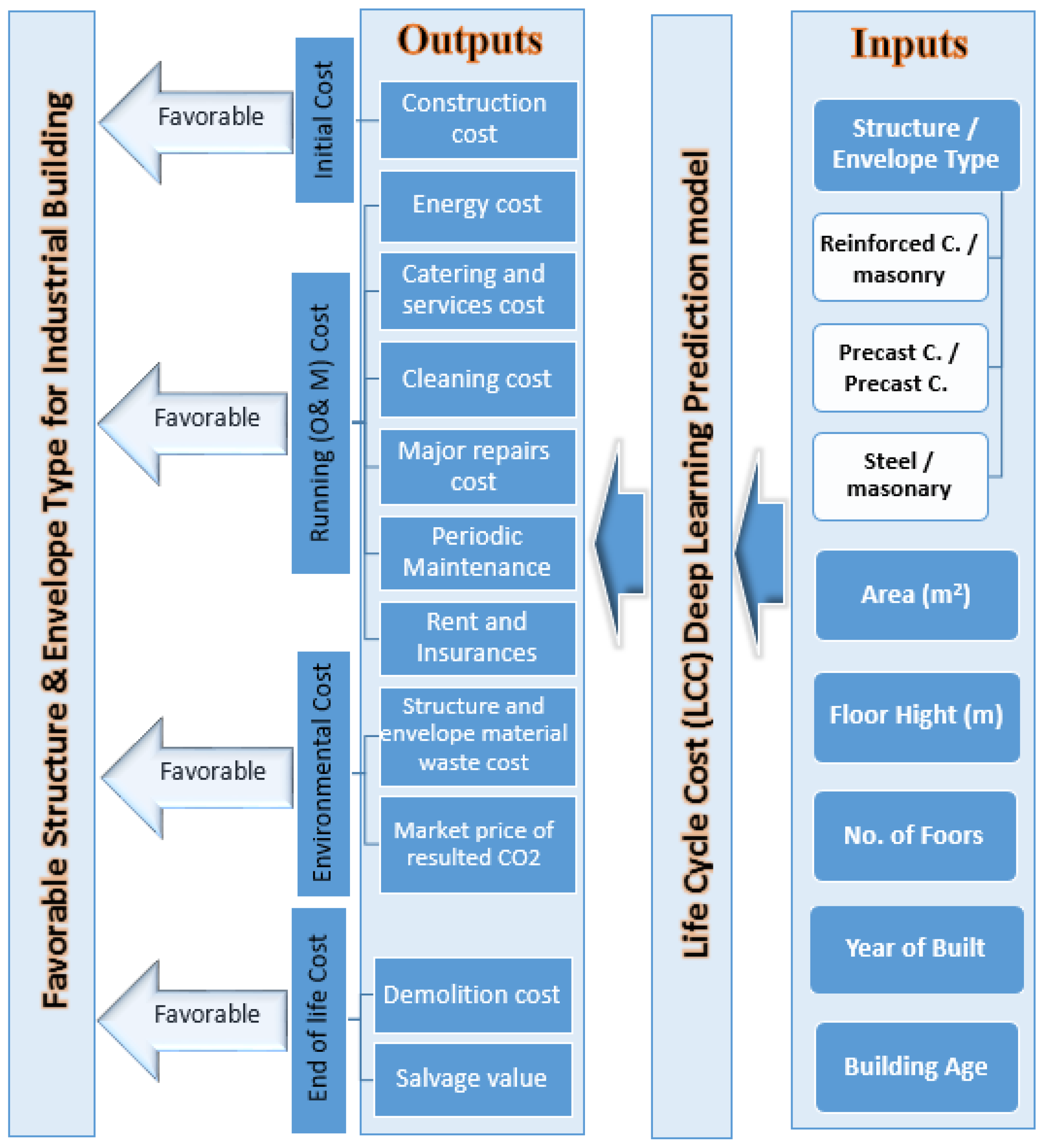
3. Methodology
3.1. Required Data for LCC Model
3.1.1. Data Preparation
3.1.2. Data Analysis
3.1.3. Data Derivation
- PVIC is the present value of the initial cost;
- IC is the amount of initial cost;
- t is the building age;
- ri is the annual inflation rate of i years ago.
- PVOM is the present value of operation and maintenance costs;
- ECj is the annual energy cost j years ago;
- C&Sj is the annual catering and services cost j years ago;
- CCj is the annual cleaning cost j years ago;
- MRj is the annual major repairs cost j years ago;
- PMj is the annual periodic maintenance cost j years ago;
- R&Ij is the annual rent and insurance costs j years ago;
- n is the length of the study period in years.
- PVEIC is the present value of environmental impact cost;
- MWCj is the annual structure and envelope material waste cost j years ago;
- Rco2j is the annual market price of resulting CO2 j years ago.
- PVEoLC is the present value of end-of-life cost;
- DCj is the annual demolition cost j years ago;
- RVj is the annual residual value cost j years ago.
3.2. Development of the LCC Deep Learning Prediction Model
- The inference problem: Inferring the configurations of the unobserved parameters.
- The learning problem: Adjusting the connections between variables of the network to be more likely to produce the desired results.
- A sigmoid belief net is formed when binary stochastic neurons are coupled in a directed acyclic graph.
- A Boltzmann machine is created when binary stochastic neurons are coupled utilizing symmetric connections.
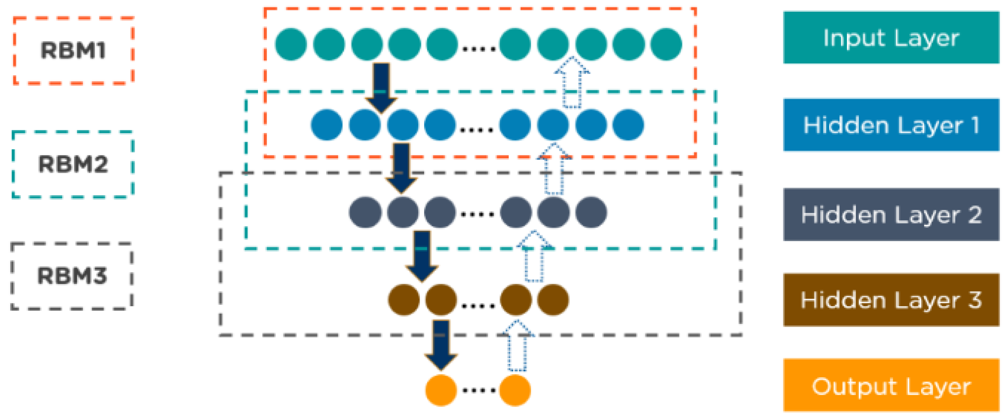
3.2.1. Configuration of the Deep Belief Network (DBN)
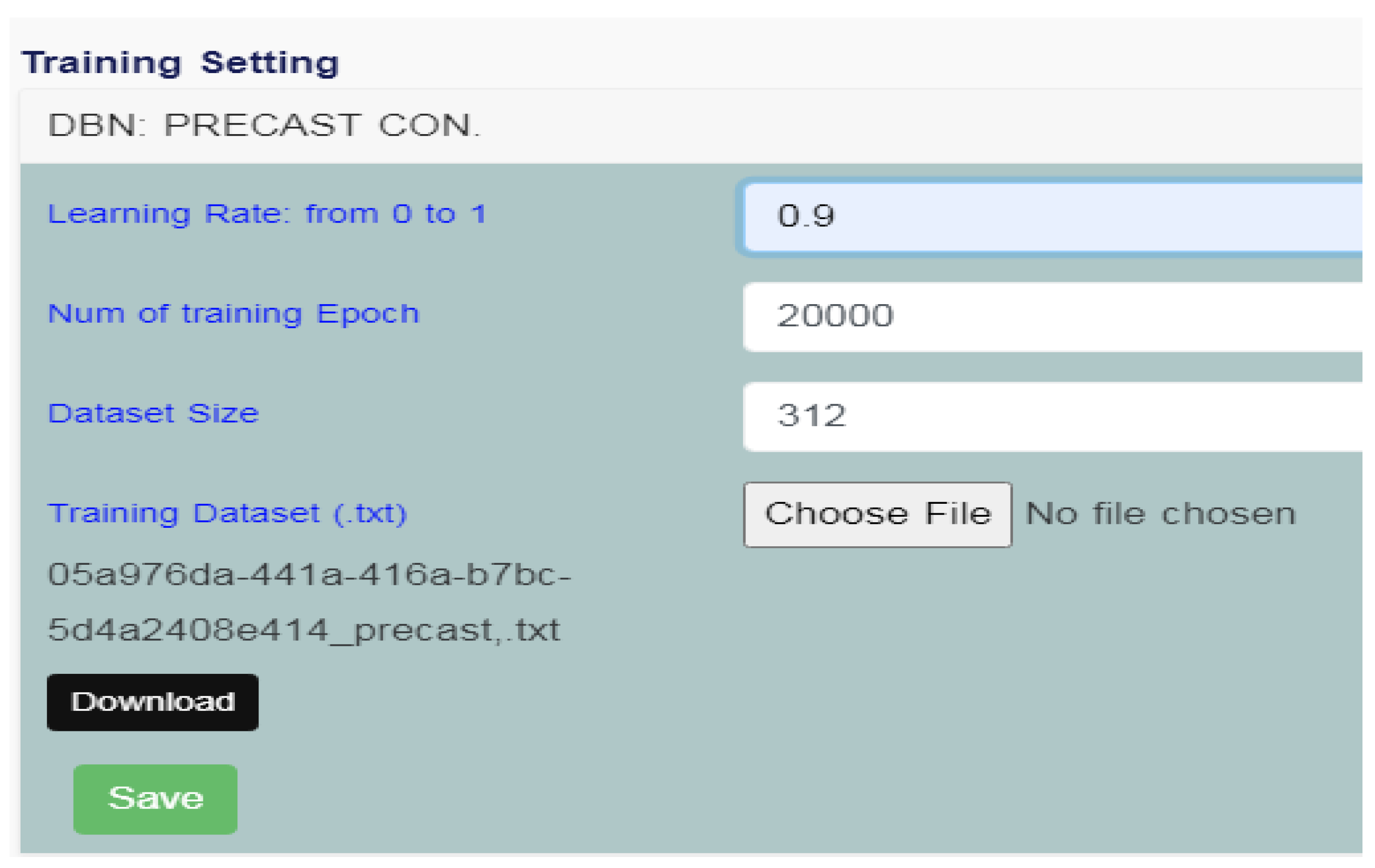
3.2.2. Training of the Network
- DBNs are trained using greedy learning methods. For learning the top-down, generative weights, the greedy learning algorithm employs a layer-by-layer approach [9].
- On the top two buried layers, the DBNs follow Gibbs sampling steps. The RBM described by the top two hidden layers is sampled in this stage.
- DBNs use a single pass of ancestral sampling through the rest of the model to generate a sample from the visible units.
- DBNs learn that the values of the latent variables in each layer can be inferred using a single bottom-up pass.
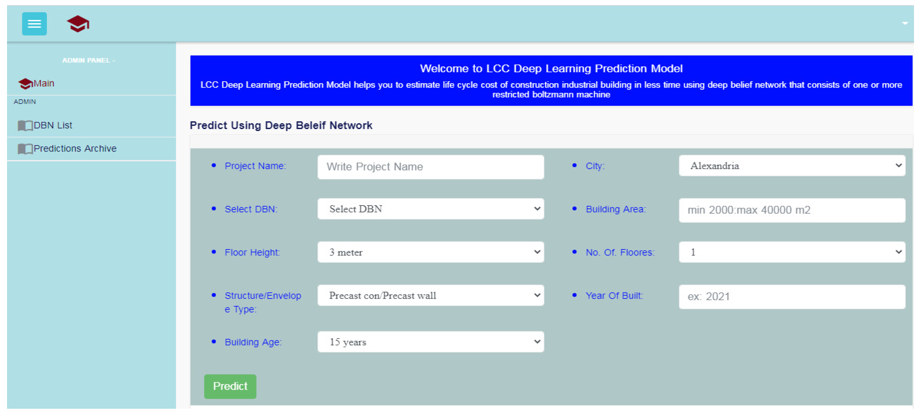
3.2.3. Predicted Values of LCC Parameters from DBN Input Simulations
4. Validation and Implementation with Case Study
4.1. Validation of the Network
4.1.1. Descriptive Statistics
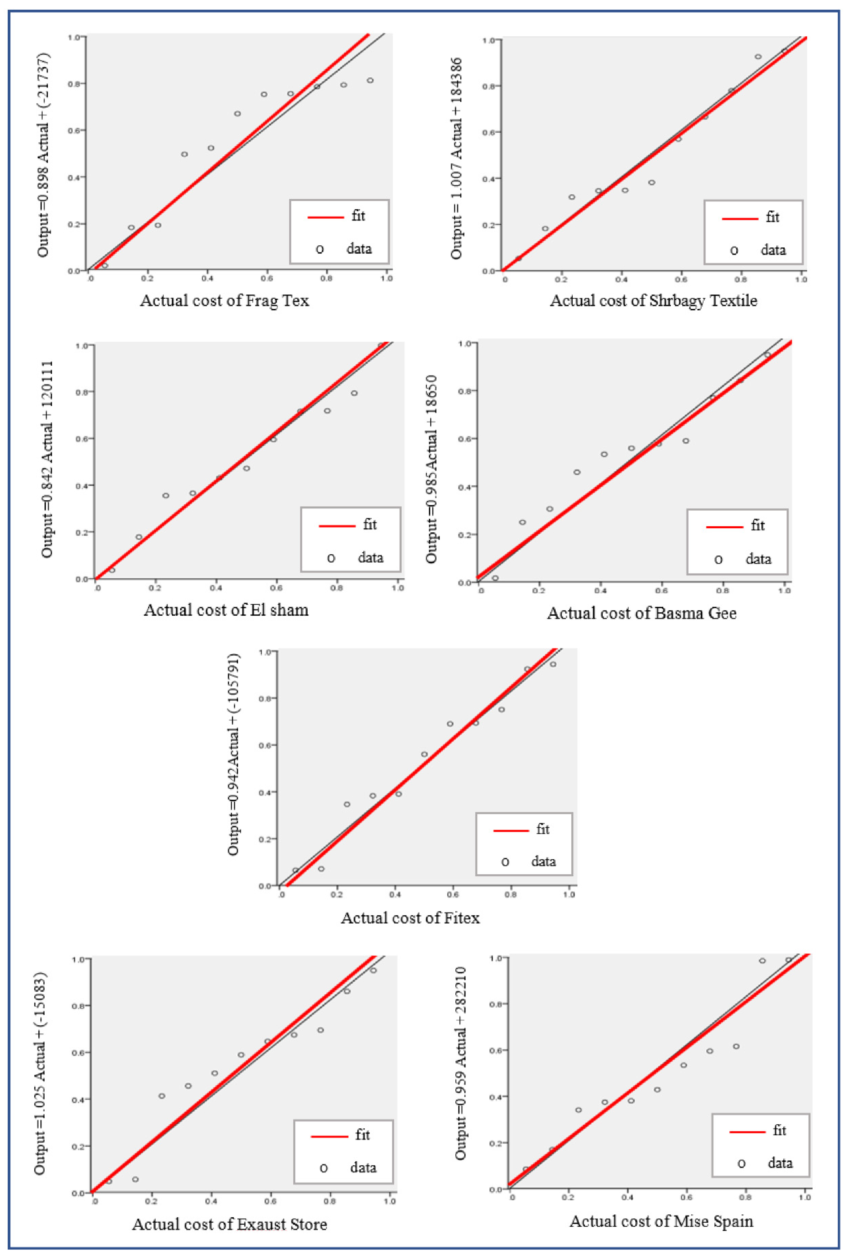
4.1.2. Regression and Mean Square Error Results
4.1.3. Autocorrelation Test (Durbin–Watson)
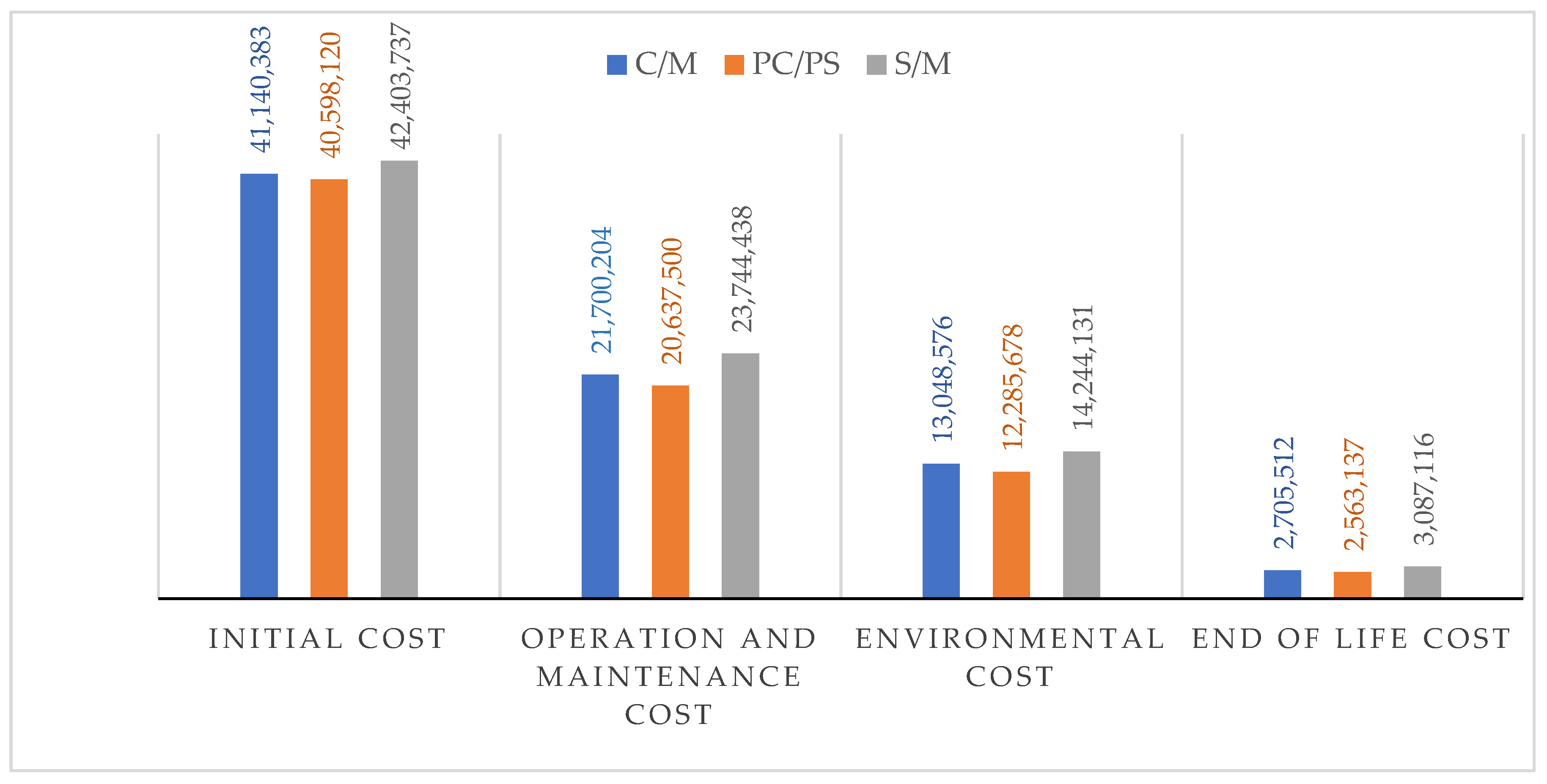
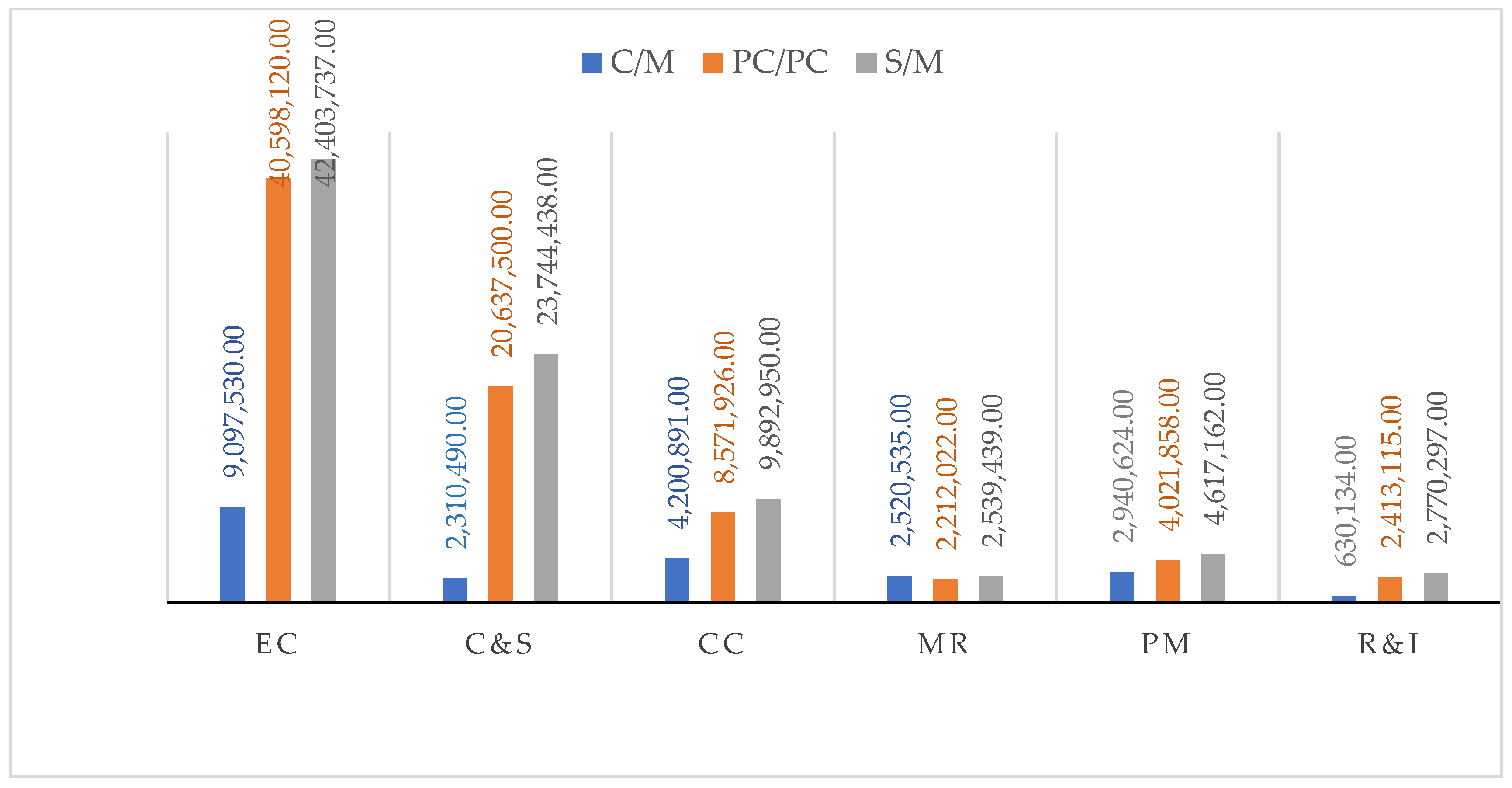
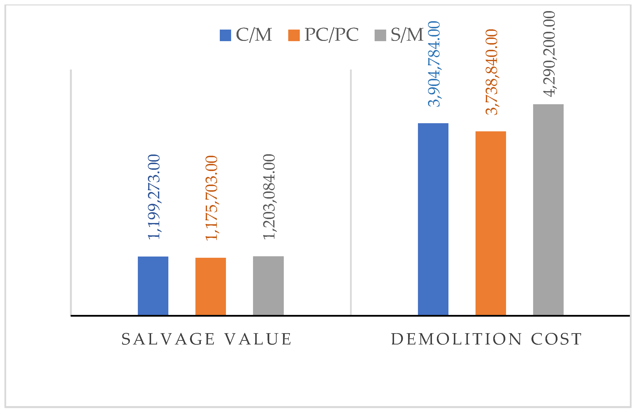
4.2. Implementation with a Case Study
5. Results
6. Discussion
7. Conclusions
Author Contributions
Funding
Institutional Review Board Statement
Informed Consent Statement
Data Availability Statement
Acknowledgments
Conflicts of Interest
References
- ISO 15686-5:2017; Buildings and Constructed Assets—Service Life Planning-Part 5: Life Cycle Costing. ISO International Organization for Standardization: Geneva, Switzerland, 2017. Available online: https://www.iso.org/standard/61148.html (accessed on 1 July 2017).
- Green Labs. Sustainability. Available online: https://sustainability.wustl.edu/get-involved/staff-faculty/green-labs-2/ (accessed on 24 November 2020).
- Rahim, M.S.; Haron, N.A. Construction cost comparison between conventional and formwork system for condominium project. Int. J. Adv. Stud. Comput. Sci. Eng. 2013, 2, 19. [Google Scholar]
- Deng, H.F.; Fannon, D.; Eckelman, M.J. Predictive modeling for US commercial build-ing energy use: A comparison of existing statistical and machine learning algorithms using CBECS microdata. Energy Build. 2018, 163, 34–43. [Google Scholar] [CrossRef]
- Dursun, O.; Stoy, C. Conceptual Estimation of Construction Costs Using the Multistep Ahead Approach. J. Constr. Eng. Manag. 2016, 142, 9. [Google Scholar] [CrossRef]
- Hong, T.; Hyun, C.; Moon, H. CBR-based cost prediction model-II of the design phase for multi-family housing projects. Expert Syst. Appl. 2011, 38, 2797–2808. [Google Scholar] [CrossRef]
- Kelleher, J.D.; Namee, B.M.; D’Arcy, A. Fundamentals of Machine Learning for Predictive Data Analytics: Algorithms, Worked Examples, and Case Studies; MIT Press: Cambridge, MA, USA, 2015. [Google Scholar]
- SAS. Machine Learning: What It Is & Why It Matters; 2018. Available online: https://www.sas.com/it_it/insights/analytics/machine-learning.htmlCost (accessed on 24 January 2019).
- Simplilearn. Available online: https://www.simplilearn.com (accessed on 21 February 2022).
- Flanagan, R.; Norman, G.; Meadows, J.; Robinson, G. Life Cycle Costing Theory and Practice, 1st ed.; BSP Professional Books: Oxford, UK, 1989; ISBN 0-632-02578-6. [Google Scholar]
- Dell’lsola, A.J.; Kirk, S.J. Life Cycle Costing for Facilities, 1st ed.; Reed Construction Data Inc.: Norwell, MA, USA, 2003; ISBN 0-87629720-5. [Google Scholar]
- Christian, J.; Pandeya, A. Cost predictions of facilities. J. Manag. Eng. 1997, 13, 52–61. [Google Scholar] [CrossRef]
- Reisinger, J.; Kugler, S.; Kovacic, I.; Knoll, M. Parametric Optimization and Decision Support Model Framework for Life Cycle Cost Analysis and Life Cycle Assessment of Flexible Industrial Building Structures Integrating Production Planning. Buildings 2022, 12, 162. [Google Scholar] [CrossRef]
- Li, C.S.; Guo, S.J. Life cycle cost analysis of maintenance costs and budgets for university buildings in Taiwan. J. Asian Archit. Build. Eng. 2012, 11, 87–94. [Google Scholar] [CrossRef] [Green Version]
- Noshadravan, A.; Miller, T.R.; Gregory, J.G. A Lifecycle Cost Analysis of Residential Buildings Including Natural Hazard Risk. J. Constr. Eng. Manag. 2017, 143, 10. [Google Scholar] [CrossRef]
- Im, H.; Srinivasan, R.S.; Maxwell, D.; Steiner, R.L.; Karmakar, S. The Impact of Climate Change on a University Campus’ Energy Use: Use of Machine Learning and Building Characteristics. Buildings 2022, 12, 108. [Google Scholar] [CrossRef]
- Godoy-Shimizu, D.; Steadman, P.; Hamilton, I.; Donn, M.; Evans, S.; Moreno, G.; Shayesteh, H. Energy Use and Height in Office Buildings. Build. Res. Inf. 2018, 46, 845–863. [Google Scholar]
- Ahmed, S.; Arocho, I. Analysis of cost comparison and effects of change orders during construction: Study of a mass timber and a concrete building project. J. Build. Eng. 2021, 33, 101856. [Google Scholar] [CrossRef]
- Tsai, W.-H.; Yang, C.-H.; Chang, J.-C.; Lee, H.-L. An Activity-Based Costing decision model for life cycle assessment in green building projects. Eur. J. Oper. Res. 2014, 238, 607–619. [Google Scholar] [CrossRef]
- An, S.-H.; Kim, G.-H.; Kang, K.-I. A case-based reasoning cost estimating model using experience by analytic hierarchy process. Build. Environ. 2007, 42, 2573–2579. [Google Scholar] [CrossRef]
- Kim, G.-H.; An, S.-H.; Kang, K.-I. Comparison of construction cost estimating models based on regression analysis, neural networks, and case-based reasoning. Build. Environ. 2004, 39, 1235–1242. [Google Scholar] [CrossRef]
- Kim, G.-H.; Yoon, J.-E.; An, S.-H.; Cho, H.-H.; Kang, K.-I. Neural network model incorporating a genetic algorithm in estimating construction costs. Build. Environ. 2004, 39, 1333–1340. [Google Scholar] [CrossRef]
- Koo, C.; Hong, T.; Hyun, C. The development of a construction cost prediction model with improved prediction capacity using the advanced CBR approach. Expert Syst. Appl. 2011, 38, 8597–8606. [Google Scholar] [CrossRef]
- Cheng, M.-Y.; Tsai, H.-C.; Hsieh, W.-S. Web-based conceptual cost estimates for construction projects using Evolutionary Fuzzy Neural Inference Model. Autom. Constr. 2009, 18, 164–172. [Google Scholar] [CrossRef]
- Jin, R.; Han, S.; Hyun, C.; Cha, Y. Application of Case-Based Reasoning for Estimating Preliminary Duration of Building Projects. J. Constr. Eng. Manag. 2016, 142, 04015082. [Google Scholar] [CrossRef]
- Robinson, C.; Dilkina, B.; Hubbs, J.; Zhang, W.; Guhathakurta, S.; Brown, M.A.; Pendyala, R.M. Machine learning approaches for estimating commercial building energy consumption. Appl. Energy 2017, 208, 889–904. [Google Scholar] [CrossRef]
- Zhang, C.; Cao, L.W.; Romagnoli, A. On the feature engineering of building energy data mining. Sustain. Cities Soc. 2018, 39, 508–518. [Google Scholar] [CrossRef]
- WBDG PBS-P100. (GSA)—Chapter 1.8—Life-Cycle Costing. In Facilities Standards for the Public Buildings Service; United States Courthouse: Seattle, WA, USA, 2005. [Google Scholar]
- Al-busaad, S.A. Assessment of Application of Life Cycle Cost on Construction Projects. Master’s Thesis, King Fahd University of Petroleum and Minerals, Dhahran, Saudi Arabia, October 1997. [Google Scholar]
- Assaf, S.; Al-Hammad, A.; Jannadi, O.A.; Abu Saad, S. Assessment of the problems of application of life cycle costing in construction projects. Cost Eng. Morgant. 2002, 44, 17–22. [Google Scholar]
- Fretty, P. Long Term Planning Helps Maximize Maintenance. PEM 2003, 27, 33. [Google Scholar]
- Khanduri, A.C.; Bedard, C.; Alkass, S. Assessing Office Building Life Cycle Costs at Preliminary Design Stage. Struct. Eng. Rev. 1996, 8, 105–114. [Google Scholar]
- Liu, Y. A Forecasting Model for Maintenance and Repair Cost for Office Building. Master’s Thesis, Concordia University, Montreal, QC, Canada, September 2006. [Google Scholar]
- Zhang, K. Life Cycle Costing for Office Buildings in Canada. Master’s Thesis, Concordia University, Montreal, QC, Canada, 1999. [Google Scholar]
- Salem, O.; Abou Rizk, S.; Ariaratnam, S. Risk-based Life Cycle Costing of Infrastructure Rehabilitation and Construction Alternatives. Am. Soc. Civ. Eng. J. Infrastruct. Syst. 2003, 9, 6–15. [Google Scholar] [CrossRef]
- El-Diraby, T.E.; Rasic, I. Framework for Managing Life-Cycle Cost of Smart Infrastructure Systems. Am. Soc. Civ. Eng. J. Comput. Civ. Eng. 2004, 18, 115–119. [Google Scholar] [CrossRef]
- Zayed, T.; Chang, L.; Fricker, J. Life-Cycle Cost Based Maintenance Plan for Steel Bridge Protection Systems. J. Perform. Constr. Facil. Am. Soc. Civ. Eng. 2002, 16, 55–62. [Google Scholar] [CrossRef]
- Asamoah, R.O.; Ankrah, J.S.; Offei-Nyako, K.; Tutu, E.O. Cost analysis of precast and cast-in-place concrete construction for selected public buildings in Ghana. J. Constr. Eng. 2016, 2016, 8785129. [Google Scholar] [CrossRef] [Green Version]
- Moussatche, H.; Languell, J. Floor Materials Life—Costing for Educational Facilities; MCB University Press: Bingley, UK, 2001; Volume 19, pp. 333–343. ISSN 0263-2772. [Google Scholar]
- Fretwell, P.L. The Design of a System for The Implementation of Life Cycle Costing for Educational Buildings in Alabama. Bachelor’s Thesis, Auburn University, Auburn, AL, USA, 1984. [Google Scholar]
- Alshamrani, O. Evaluation of School Buildings Using Sustainability Measures and Life-Cycle Costing Technique. Ph.D. Thesis, Concordia University, Montréal, QC, Canada, 2012. [Google Scholar]
- Norman, G. Life Cycle Costing. Prop. Manag. 1990, 8, 344–356. [Google Scholar] [CrossRef]
- Kishk, M.; Al-Hajj, A. An integrated framework for life cycle costing in buildings. In Proceedings of the COBRA 1999 RICS Construction and Building Research Conference, Glasgow, UK, 1 September 1999; Volume 2, pp. 92–101. [Google Scholar]
- Rodrigues, V.; Martins, A.A.; Nunes, M.I.; Quintas, A.; Mata, T.M.; Caetano, N. LCA of constructing an industrial building: Focus on embodied carbon and energy. Energy Procedia 2018, 153, 420–425. [Google Scholar] [CrossRef]
- Marrero, M.; Rivero-Camacho, C.; Martínez-Rocamora, A.; Alba-Rodríguez, M.D.; Solís-Guzmán, J. Life Cycle Assessment of Industrial Building Construction and Recovery Potential. Case Studies in Seville. Processes 2022, 10, 76. [Google Scholar] [CrossRef]
- Opher, T.; Duhamel, M.; Posen, I.D.; Panesar, D.K.; Brugmann, R.; Roy, A.; Zizzo, R.; Sequeira, L.; Anvari, A.; MacLean, H.L. Life cycle GHG assessment of a building restoration: Case study of a heritage industrial building in Toronto, Canada. J. Clean. Prod. 2021, 279, 123819. [Google Scholar] [CrossRef]
- Weerasinghe, A.S.; Ramachandra, T.; Rotimi, J.O.B. Comparative life-cycle cost (LCC) study of green and traditional industrial buildings in Sri Lanka. Energy Build. 2021, 234, 110732. [Google Scholar] [CrossRef]
- Kovacic, I.; Waltenbereger, L.; Gourlis, G. Tool for life cycle analysis of facade-systems for industrial buildings. J. Clean. Prod. 2016, 130, 260–272. [Google Scholar] [CrossRef]
- Reisinger, J.; Knoll, M.; Kovacic, I. Design space exploration for flexibility assessment and decision making support in integrated industrial building design. Optim. Eng. 2021, 22, 1693–1725. [Google Scholar] [CrossRef]
- Van der Maas, H.L.J.; Snoek, L.; Stevenson, C.E. How much intelligence is there in artificial intelligence? A 2020 Update. Intelligence 2021, 87, 101548. [Google Scholar] [CrossRef]
- Zeba, G.; Dabić, M.; Čičak, M.; Daim, T.; Yalcin, H. Technology mining: Artificial intelligence in manufacturing. Technol. Forecast. Soc. Change 2021, 171, 120971. [Google Scholar] [CrossRef]
- Chen, C.; Hu, Y.; Karuppiah, M.; Kumar, P.M. Artificial intelligence on economic evaluation of energy efficiency and renewable energy technologies. Sustain. Energy Technol. Assess. 2021, 47, 121358. [Google Scholar] [CrossRef]
- Sircar, A.; Yadav, K.; Rayavarapu, K.; Bist, N.; Oza, H. Application of machine learning and artificial intelligence in oil and gas industry. Pet. Res. 2021, 6, 379–391. [Google Scholar] [CrossRef]
- Ruggieri, S.; Cardellicchio, A.; Leggieri, V.; Uva, G. Machine-learning based vulnerability analysis of existing buildings. Autom. Constr. 2021, 132, 103936. [Google Scholar] [CrossRef]
- Cardellicchio, A.; Ruggieri, S.; Leggieri, V.; Uva, G. View VULMA: Data Set for Training a Machine-Learning Tool for a Fast Vulnerability Analysis of Existing Buildings. Data 2022, 7, 4. [Google Scholar] [CrossRef]
- Khallaf, R.; Khallaf, M. Classification and analysis of deep learning applications in construction: A systematic literature review. Autom. Constr. 2021, 129, 103760. [Google Scholar] [CrossRef]
- Akinosho, T.D.; Oyedele, L.O.; Bilal, M.; Ajayi, A.O.; Delgado, M.D.; Akinade, O.O.; Ahmed, A.A. Deep learning in the construction industry: A review of present status and future innovations. J. Build. Eng. 2020, 32, 101827. [Google Scholar] [CrossRef]
- Mocanu, E.; Nguyen, P.H.; Gibescu, M.; Kling, W.L. Deep learning for estimating building energy consumption. Sustain. Energy Grids Netw. 2016, 6, 91–99. [Google Scholar] [CrossRef]
- Fan, C.; Xiao, F.; Zhao, Y. A short-term building cooling load prediction method using deep learning algorithms. Appl. Energy 2017, 195, 222–233. [Google Scholar] [CrossRef]
- Singaravel, S.; Suykens, J.; Geyer, P. Deep-learning neural-network architectures and methods: Using component-based models in building-design energy prediction. Adv. Eng. Inf. 2018, 38, 81–90. [Google Scholar] [CrossRef]
- Egyptian Engineers Syndicate. Available online: https://eea.org.eg/ (accessed on 4 March 2022).
- Egyptian Environment Industry, 2021–2024. Available online: https://www.reportlinker.com/report-summary/Environmental-Services/114089/Egyptian-Environment-Industry.html?tstv=no-test (accessed on 4 March 2022).
- Point Carbon Website. Available online: https://www.refinitiv.com/en/products/point-carbon-prices (accessed on 4 March 2022).
- Maury-Ramírez, A.; Illera-Perozo, D.; Mesa, J.A. Circular Economy in the Construction Sector: A Case Study of Santiago de Cali (Colombia). Sustainability 2022, 14, 1923. [Google Scholar] [CrossRef]
- Egypt Inflation Rate. (1960–2021). Available online: https://www.macrotrends.net/countries/EGY/egypt/inflation-rate-cpi (accessed on 4 March 2022).
- Gao, X.; Pishdad-Bozorgi, P. A framework of developing machine learning models for facility life-cycle cost analysis. Build. Res. Inf. 2020, 48, 501–525. [Google Scholar] [CrossRef]
- Geoffrey, E.; Hinto, N.; Osindero, S.; Theh, Y.-W. A fast learning algorithm for deep belief nets. Neural Comput. 2006, 7, 1527–1554. [Google Scholar] [CrossRef]
- Advanced Concrete Products (ACP). Performance of Pre-Cast versus Cast-in-Place Concrete Retrieved. 2014. Available online: http://www.advanceconcreteproducts.com/1/acp/precast_vs_cast_in_place.asp (accessed on 4 March 2022).
- Marceau, M.L.; Bushi, L.; Meil, J.K.; Bowick, M. Life Cycle Assessment for Sustainable Design of Precast Concrete Commercial Buildings in Canada. In Proceedings of the 1st International Specialty Conference on Sustaining Public Infrastructure, Edmonton, AB, USA, 6–9 June 2012. [Google Scholar]
- Wang, S.; Sinha, R. Life Cycle Assessment of Different Prefabricated Rates for Building Construction. Buildings 2021, 11, 552. [Google Scholar] [CrossRef]
- Tumminia, G.; Guarino, F.; Longo, S.; Mistretta, M.; Cellura, M.; Aloisio, D.; Antonucci, V. Life cycle energy performances of a Net Zero Energy prefabricated building in Sicily. Energy Procedia 2017, 140, 486–494. [Google Scholar] [CrossRef]
- Achenbach, H.; Wenker, J.L.; Rüter, S. Life cycle assessment of product-and construction stage of prefabricated timber houses: A sector representative approach for Germany according to EN 15804, EN 15978 and EN 16485. Eur. J. Wood Wood Prod. 2018, 76, 711–729. [Google Scholar] [CrossRef]
- Wen, T.J.; Siong, H.C.; Noor, Z.Z. Assessment of embodied energy and global warming potential of building construction using life cycle analysis approach: Case studies of residential buildings in Iskandar Malaysia. Energy Build. 2015, 93, 295–302. [Google Scholar] [CrossRef]


| Alternatives | Frame Type | Wall Type | Floor Type | Roof Type |
|---|---|---|---|---|
| C/M | Reinforced concrete | Masonry | Solid concrete slab | Solid concrete slab |
| PC/PS | Precast/pre-stressed | Precast concrete panels | Pre-stressed slab | Hollow core slab |
| S/M | Steel frame | Masonry | Concrete/metal deck/open joists | Concrete/metal deck on open web joists |
| Selected Criteria | Descriptions | Data Preparation | |
|---|---|---|---|
| Inputs | Building area | The total area of the building, which is one of the basics of the building footprint. | The capital planning and investment control system. Some digital spreadsheets that record the design and construction costs from manufactories such as Modern4concrete in Egypt. |
| Floor height | The height of each building story in unit length, which is one of the basics of the building footprint. | ||
| Numbers of floors | Number of building stories (e.g., 1, 2, 3, …), which is one of the basics of the building footprint. | ||
| Structure and envelope type | These include steel, concrete, wood, and precast concrete, in various combinations. | ||
| Building age | The study period, in years (e.g., 15, 25, 30, … years). | ||
| Year of construction | This parameter includes the projects built within the study period. | ||
| Outputs | Initial Cost (IC) | Construction Cost | |
| Operation and Maintenance Cost (O&M) | This refers to hard facility-management costs These costs include operating costs such as cleaning and energy costs, maintenance costs, and other costs [1,2]. | Computerized maintenance management systems of industrial boards of construction companies in Egypt. | |
| Energy Cost (EC) | Energy used for heating and lighting [27]. | From standard energy and simulation. The building energy management systems. | |
| Catering and Services (C&S) | General support services, communications and security services, letting fees, facilities management fees, caretaker and janitorial services, service transport, IT services, and laundry and linen services, e.g., internal deliveries [1]. | From the industrial boards of construction companies, such as the Modern4concrete industrial board in Egypt. | |
| Cleaning (C) | Waste management and disposal. | ||
| Major Repairs (MR) | Redecoration, renovation, rehabilitation, and replacement. | ||
| Periodic Maintenance (PM) | The cost of contractors who perform skilled jobs, such as the sanitation and HVAC services [1]. | ||
| Rent and Insurance (R&I) | Insurance rates and other local taxes and charges. | ||
| Environmental Impact Cost (EIC) | The environmental cost refers to the cost of controlling gas emissions, and of structural and envelope material waste costs [41]. | From environmental impact estimators in Egypt [62]. | |
| Structure and envelope Material Waste Cost (MWC) | Waste gathered from all stages, such as production of raw materials, manufacturing of concrete, placing concrete at the location, and demolition. | From the industrial boards of construction companies and their computerized maintenance management systems. | |
| Market price of resulting CO2 (RCO2) | Cost of controlling gas emissions. | From the carbon market (Point Carbon website) [63]. | |
| End-of-Life Cost (EoLC) | This includes disposal and demolition, but specifically includes the worth of alternatives at the end period of LCCA [64]. | The capital planning and investment control system. Some digital spreadsheets that record the design and construction costs. Some physical documents related to building design and construction. | |
| Residual Value (RV) or Salvage Value (SV) | Salvage value, recycling, the conversion of waste from the building into new objectives. | ||
| Demolition cost (DC) | Building demolition waste such as materials, aggregates, concrete, wood, and metal. |
| Basic Statistics | Area (m2) | Floor Height (m) | Number of Floors | Structure and Envelope Type | Building Age (Years) | Year of Construction | Initial Cost (LE) |
|---|---|---|---|---|---|---|---|
| Maximum | 40,000 | 8 | 5 | 1 | 20 | 2020 | 43,172,350 |
| Minimum | 820 | 3 | 1 | 1 | 1 | 2000 | 3,261,480 |
| Mean | 18,052 | 5.2 | 3 | 1 | 11.3 | 2013 | 17,005,149 |
| Median | 16,200 | 5 | 3 | 1 | 13 | 2015 | 15,582,100 |
| No. | Project Name | City | Input Building Parameter | ||
|---|---|---|---|---|---|
| Area (m2) | Floor Height (m) | Number of Floors | |||
| 1 | Frag Tex | 10th of Ramadan | 13,435 | 8 | 1 |
| 2 | Shrbagy Textile | 10th of Ramadan | 11,560 | 5 | 3 |
| 3 | El sham | El Obour | 16,100 | 3 | 5 |
| 4 | Basma Gee | 10th of Ramadan | 7784 | 8 | 1 |
| 5 | Fitex | 10th of Ramadan | 11,344 | 6 | 2 |
| 6 | Mise Spain Soinng factory | Sadat city | 38,388 | 5 | 3 |
| 7 | Exaust Store Robaeia | Sadat city | 4672 | 8 | 1 |
| Actual Values of Buildings’ LCC in 2021 (EGP) | ||||||||
|---|---|---|---|---|---|---|---|---|
| Project Name | Frag Tex Factory | Shrbagy Textile Factory | El Sham Factory | Basma Gee Factory | Fitex Factory | Mise Spain Soinng Factory | Exaust Store Robaeia | |
| IC | 15,450,250 | 22,831,000 | 26,967,500 | 7,394,800 | 20,702,800 | 40,891,065 | 4,947,413 | |
| O&M Cost | EC | 2,410,509 | 3,545,335 | 4,228,111 | 1,178,026 | 3,240,058 | 6,385,139 | 774,764 |
| C&S | 665,865 | 987,217 | 1,166,355 | 315,457 | 841,566 | 1,736,051 | 213,060 | |
| CC | 1,201,755 | 1,727,667 | 2,131,555 | 574,013 | 1,651,029 | 3,190,820 | 387,382 | |
| MR | 725,553 | 1,072,600 | 1,260,933 | 342,408 | 972,318 | 1,916,692 | 232,429 | |
| PM | 842,828 | 1,255,367 | 1,478,689 | 405,409 | 1,134,720 | 2,237,974 | 271,167 | |
| R&I | 181,063 | 268,950 | 316,233 | 86,352 | 247,154 | 473,923 | 58,107 | |
| EIC | MWC | 1,048,129 | 1,439,723 | 1,709,629 | 452,511 | 1,392,858 | 2,612,683 | 322,818 |
| RCO2 | 2,354,301 | 3,406,020 | 4,235,802 | 1,185,858 | 3,153,001 | 6,198,260 | 753,243 | |
| EoL | SV | 442,057 | 652,099 | 762,058 | 216,449 | 620,381 | 1,162,526 | 143,474 |
| DC | 1,160,143 | 1,525,248 | 1,923,144 | 542,123 | 1,530,953 | 2,976,314 | 358,687 | |
| Predicted Values LCC of Buildings’ after 30 Years (EGP) from the Year of 1991 | ||||||||
|---|---|---|---|---|---|---|---|---|
| Project Name | Frag Tex | Shrbagy Textile | El Sham | Basma Gee | Fitex | Mise Spain Soinng Factory | Exaust Store Robaeia | |
| IC | 13,844,146 | 23,099,754 | 2,2787,784 | 7,296,579 | 19,416,808 | 39,286,999 | 5,061,459 | |
| O&M Cost | EC | 2,151,722 | 3,983,835 | 3,870,192 | 1,201,967 | 2,837,209 | 6,792,340 | 757,467 |
| C&S | 591,724 | 1,095,555 | 1,064,303 | 330,541 | 780,233 | 1,867,893 | 208,303 | |
| CC | 1,075,861 | 1,991,918 | 1,935,096 | 600,984 | 1,418,605 | 3,396,170 | 378,733 | |
| MR | 645,517 | 1,195,151 | 1,161,058 | 360,590 | 851,163 | 2,037,702 | 227,240 | |
| PM | 753,103 | 1,394,342 | 1,354,567 | 420,689 | 993,023 | 2,377,319 | 265,113 | |
| R&I | 161,379 | 298,788 | 290,264 | 90,148 | 212,791 | 509,426 | 56,810 | |
| EIC | MWC | 896,551 | 1,659,931 | 1,612,580 | 500,820 | 1,182,170 | 2,830,142 | 315,611 |
| RCO2 | 2,091,952 | 3,873,173 | 3,762,687 | 1,168,579 | 2,758,398 | 6,603,664 | 736,426 | |
| EoL | SV | 321,260 | 564,525 | 577,593 | 176,410 | 485,232 | 1,074,311 | 149,914 |
| DC | 996,168 | 1,844,368 | 1,791,756 | 556,466 | 1,313,523 | 3,144,602 | 350,679 | |
| Error Ratio % | 3.60 | 3.47 | 3.20 | 3.53 | 3.64 | 3.82 | 3.31 | |
| Frag Tex | Shrbagy Textile | El Sham | Basma Gee | Fitex | Mise Spain Soinng Factory | Exaust Store Robaeia | |
|---|---|---|---|---|---|---|---|
| Mean | 2,139,035 | 3,727,394 | 3,655,261 | 1,154,888 | 2,931,741 | 6,356,415 | 773,432 |
| Standard Deviation | 3,933,869 | 6,532,598 | 6,447,773 | 2,067,754 | 5,530,462 | 11,103,635 | 1,439,142 |
| Frag Tex | Shrbagy Textile | El Sham | Basma Gee | Fitex | Mise Spain Soinng Factory | Exaust Store Robaeia | |
|---|---|---|---|---|---|---|---|
| R | 1.00 | 0.996 | 0.998 | 1.00 | 0.997 | 0.998 | 0.995 |
| Mean Square Error E14 | 1.547 | 4.260 | 4.156 | 0.427 | 3.058 | 12.30 | 0.207 |
| Frag Tex | Shrbagy Textile | El Sham | Basma Gee | Fitex | Mise Spain Soinng Factory | Exaust Store Robaeia | |
|---|---|---|---|---|---|---|---|
| Durbin–Watson | 1.138 | 2.969 | 2.790 | 2.118 | 2.599 | 2.735 | 2.833 |
| Parameter | Description | Parameter | Description |
|---|---|---|---|
| Industry name | El Mahalla Spinning | City | El Mahalla |
| Area | 53,398 (m2) | Number of floors | 1 |
| Floor height | 8 (m) | Structure type | Test all |
| Lifespan | 30 years | Year of construction | 2019 |
| C/M | PC/PS | S/M | |||||
|---|---|---|---|---|---|---|---|
| Initial Cost (IC) | 41,140,383 | 40,598,120 | 42,403,737 | ||||
| O&M Cost | EC | 9,097,530 | 21,700,204 | 8,571,926 | 20,637,500 | 9,892,950 | 23,744,438 |
| C&S | 2,310,490 | 2,212,022 | 2,539,439 | ||||
| CC | 4,200,891 | 4,021,858 | 4,617,162 | ||||
| MR | 2,520,535 | 2,413,115 | 2,770,297 | ||||
| PM | 2,940,624 | 2,815,301 | 3,232,014 | ||||
| R&I | 630,134 | 603,279 | 692,574 | ||||
| EIC | MWC | 3,914,573 | 13,048,576 | 3,685,694 | 12,285,678 | 4,273,239 | 14,244,131 |
| RCO2 | 9,134,003 | 8,599,953 | 9,970,892 | ||||
| EoLC | SV | 1,199,273 | 2,705,512 | 1,175,703 | 2,563,137 | 1,203,084 | 3,087,116 |
| DC | 3,904,784 | 3,738,840 | 4,290,200 | ||||
| Total LCC (EGP) | 78,594,676 | 76,084,405 | 83,479,422 | ||||
| Error Ratio % | 5.05 | 5.03 | 4.99 | ||||
Publisher’s Note: MDPI stays neutral with regard to jurisdictional claims in published maps and institutional affiliations. |
© 2022 by the authors. Licensee MDPI, Basel, Switzerland. This article is an open access article distributed under the terms and conditions of the Creative Commons Attribution (CC BY) license (https://creativecommons.org/licenses/by/4.0/).
Share and Cite
Meshref, A.; El-Dash, K.; Basiouny, M.; El-Hadidi, O. Implementation of a Life Cycle Cost Deep Learning Prediction Model Based on Building Structure Alternatives for Industrial Buildings. Buildings 2022, 12, 502. https://doi.org/10.3390/buildings12050502
Meshref A, El-Dash K, Basiouny M, El-Hadidi O. Implementation of a Life Cycle Cost Deep Learning Prediction Model Based on Building Structure Alternatives for Industrial Buildings. Buildings. 2022; 12(5):502. https://doi.org/10.3390/buildings12050502
Chicago/Turabian StyleMeshref, Ahmed, Karim El-Dash, Mohamed Basiouny, and Omia El-Hadidi. 2022. "Implementation of a Life Cycle Cost Deep Learning Prediction Model Based on Building Structure Alternatives for Industrial Buildings" Buildings 12, no. 5: 502. https://doi.org/10.3390/buildings12050502
APA StyleMeshref, A., El-Dash, K., Basiouny, M., & El-Hadidi, O. (2022). Implementation of a Life Cycle Cost Deep Learning Prediction Model Based on Building Structure Alternatives for Industrial Buildings. Buildings, 12(5), 502. https://doi.org/10.3390/buildings12050502