Abstract
It is necessary to develop effective methods for visually detecting concrete damage because minor damage can affect the performance of concrete materials. However, the non-homogeneous nature of concrete materials limits the application of imaging algorithms that have been widely used in aerospace and mechanical fields; thus, obtaining high-resolution imaging maps is difficult. In this study, feasibility research on concrete damage detection was conducted using the time reversal focusing imaging algorithm. A new method for characterizing various concrete damage conditions with focusing curves was proposed. ABAQUS software was utilized to establish five types of concrete damage, and the imaging quality of the proposed method was evaluated in Python. The effect of the relative position of the damage and the sensors was analyzed. The focusing curve was extracted from the imaging area to further explain the image information. The numerical simulation results show that time reversal focusing had better damage localization than the forward algorithm; time focusing also improved the spatial focusing quality. In addition, focusing curves were used to extract information from the main lobe and to determine the size and location of the damage.
1. Introduction
Concrete is an important building material that is used in both civil and military structures, such as bridges and high-rise buildings. However, most concrete buildings have imperfections, such as cracks, holes, and honeycomb damage, due to concrete creep and shrinkage, the action of long-term loads, or abrupt disasters. These flaws have long been major concerns due to safety, operation time loss and material maintenance cost considerations. Implementing effective health diagnoses as concrete buildings age has become increasingly important. Traditional nondestructive testing methods, such as infrared thermal imaging [1], ground-penetrating radar (GPR) [2], and radiographic testing [3], have been used to locate voids in concrete. These methods require cumbersome equipment and experienced professionals to analyze measurements. Furthermore, these methods have some limitations for detecting microcracks or surface cracks in concrete structures. New high-precision, intelligent diagnosis methods need to be developed to address these issues. Yu et al. [4] used one sensor to obtain the reflection position information of concrete cracks and then combined the signals obtained from three sensors to obtain the crack width. Han et al. [5] proposed an improved Otsu method integrated with edge detection and a decision tree for crack detection. Carrasco et al. [6] proposed an automatic method to measure the width of surface cracks based on digital image processing technology and used this method to detect real cracks with widths as small as 0.15 mm.
In recent years, many researchers have investigated piezoelectric transducers in structural health diagnoses due to their low cost, quick response time, and wide frequency range [7]. Health detection technology based on piezoelectric transducers can be divided into active detection and passive detection. Active detection includes the wave propagation (WP) method and the impedance method [8]. In the wave-based method, ultrasonic waves propagate through concrete, and damage is detected by analyzing the characteristics of the received signal [9]. However, concrete damage detection based on the WP method cannot directly characterize the location and size of the damage because only the characteristics of the processed signal are analyzed [10]. Moreover, damage detection is limited to qualitative detection.
Various damage imaging methods have extended WP-based qualitative detection methods to achieve quantitative detection. Damage recognition based on an imaging algorithm can display damage as an image to visualize its location, size, and morphological characteristics of the damage [11]. At present, concrete imaging methods include computed tomography (CT) imaging, the synthetic aperture focusing technique (SAFT), the delay-and-sum (DAS) method, and time reversal imaging. Tomography has been widely used and studied in the field of medical diagnosis. In recent years, this method has been successfully extended to identify damage in engineering structures [12,13,14]. To evaluate the quality of the connection of the bond between steel and concrete, Zielińska et al. [15] proposed a new theoretical model. The results indicated that ultrasonic tomography technology has great potential for detecting debonding in reinforced concrete structures. The idea of SAFT is derived from the offset imaging technique and synthetic aperture radar imaging technique. Ganguli et al. [16] used SAFT to detect pore defects at different locations in reinforced concrete media, extending the traditional approach to synthesize images of the media using full-mode conversion of the scattered fields, resulting in a more robust sensing algorithm. The DAS method is a simple and effective imaging method for locating structural damage. In this technique, each pixel value in a grid is calculated by summing the time-of-flight amplitudes of different signals, with the maximum pixel value representing the most likely damage location. Gao et al. [17] used a circular DAS imaging algorithm to process a scattered signal and reconstruct an image of the damage, and conducted two experiments to demonstrate the effectiveness of the proposed method. Furthermore, the improved DAS imaging algorithm has been implemented on a concrete slab with eight embedded tubular piezoelectric transducers (PZTs) [18]. Alleyne et al. [19] proposed a probabilistic damage detection reconstruction algorithm based on the DAS method. The presence of defects changes the damage index (DI), and the DI can be used to calculate the probability of the presence of defects at each point in the measurement region. The reconstruction algorithm for probabilistic inspection of defects (RAPID) imaging method has been used to visualize defects using a small number of transceiver paths [20].
Due to its low signal-to-noise ratio and frequency attenuation during the concrete inspection process, new signal processing techniques are urgently needed to improve the SAFT method [21]. Additionally, current concrete imaging algorithms are limited to slab concrete and a single damage type due to the complexity of ultrasonic propagation. Zhao et al. [22] simulated concrete without steel reinforcement and used the time reversal method to identify two signal sources. The results showed that nondestructive evaluation based on time reversal can be used to locate two signal sources within concrete. Time reversal, which is used to converge and focus the wave source, has been widely used in underwater communications and aerospace engineering. The advantages of this method include its self-adapting spatial and temporal focusing characteristics [23]. In addition, this method can trace complex multipath damage signals through high-order scattering media [24]. Therefore, it is well suited for inhomogeneous media such as concrete. There are several improved time reversal algorithms, such as time reversal operator decomposition, time reversal multiple signal classification, and virtual time reversal methods [25,26,27]. These methods improve the resolution of multidamage detection. Mori et al. [28] investigated the time reversal spatial focusing quality of lamb waves and obtained damage imaging maps after the A0 and S0 modes were excited. Although some research has been conducted on time reversal focusing, the relationship between time focusing and spatial focusing is not well understood. In addition, it is worthwhile for researchers to obtain damage information from time reversal focusing curves to supplement damage information from imaging maps. To achieve a better focusing effect, many researchers have used array transducers near the focus point [29]. The focusing result varies based on the sensor arrangement. The current study focuses on a single type of damage, although the relative position of the damage and the array sensor affects the damage imaging map.
In this study, ABAQUS software was utilized to establish five types of hole damage and to simulate the relative position of the damage and the array sensor. Focusing curves were innovatively utilized to characterize different types of damage image information of concrete structures. The damage scattering signal was obtained by subtraction and reversal. Time reversal focusing imaging was realized based on Python, and the imaging results of the forward and reverse algorithms were compared. The focusing time was calculated by determining the time point corresponding to the focusing index, and the effect of time focusing on spatial focusing was analyzed based on the quality of the damage imaging. A focusing curve was used to determine the relationship between the imaging area and the focusing index to interpret different types of damage image information.
2. Ultrasound Time Reversal Focusing Imaging
Ultrasonic imaging is used to observe the internal structure of an object with a wave field with an ultrasonic frequency between 20 kHz and 200 kHz. The ultrasonic wave is excited by the excitation sensor through the concrete and received by the receiving sensor. The propagation path will change if it encounters damage, such as cracks, honeycombs, or wormholes, as it propagates through the concrete. Scattering and reflection both occur, changing the energy of the incident wave received by the receiving sensor [30], as shown in Figure 1.
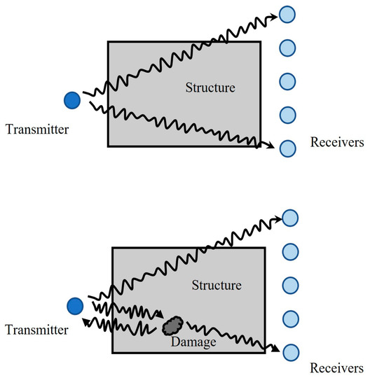
Figure 1.
The principle of ultrasonic imaging.
2.1. The Time Reversal Invariance of the Acoustic Wave Equation
When compared with traditional reconstruction algorithms, time reversal algorithms have noniterative and super resolution capabilities; thus, they have been widely used in mechanical aviation and biomedical imaging [31]. Time reversal consists of two steps: a forward propagation step and a backward propagation step. Because the linearized wave equation only includes the second derivative of the sound pressure with respect to time, as shown in Equation (1) [32], the forward propagation sound field and the backward propagation sound field radiated by the sound source are the solutions of the wave equation, thus realizing time reversal focusing.
The general solution of the one-dimensional wave equation is:
Based on the relationship between the wavenumber and the wave speed, the above formula can be simplified to:
where is the frequency, is the wavenumber, and is the wave speed.
2.2. Time Reversal Focusing Imaging
One application of the time reversal method is pulse-echo time reversal processing, which has been widely used in nondestructive evaluation and underwater target detection. In this method, the response signal is time-reversed and retransmitted through the time reversal mirror (TRM). Due to the time-reversed focusing characteristic, the signal retransmitted into the medium is focused at the target, as shown in Figure 2.
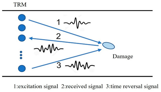
Figure 2.
Pulse-echo time reversal processing.
Let represent the location of the sensor and represent the sensor number. All receiving sensor arrays can be expressed as:
where represents the total number of sensors. During forward detection without damage, a series of displacement field signals can be obtained. The th sensor is excited, and the signal received by the th sensor can be expressed as . During forward detection with damage, similar signals can be obtained, with the signal received by the th sensor expressed as . Thus, the damage scattering signal obtained by each receiving sensor can be expressed as [17]:
2.2.1. Time Reversal of Damage Scattering Waves
The time reversal simulation process is carried out in an undamaged structure (geometric and material properties are known) after the damage scattering signal is obtained. The time reversal processing of the damage scattering signal can be expressed as:
where represents the total time. The time reversal signal is used as the excitation signal in the time reversal imaging process. N groups of time reversal signals are transmitted at the same time, forming a focusing function:
The maximum value of the focusing function is known as the focusing index [28], which occurs at the focusing point.
2.2.2. Time Reversal of Direct and Scattering Waves
The total field reverse propagation is the sum of the reverse direct field and the scattering field, with the time reversal simulation process carried out in an undamaged structure. The time reversal signal can be expressed as:
The time reverse signal is used as the excitation signal in the time reversal imaging process, and both the direct and scattering wave signals are emitted at the same time, forming a focusing function. Then, the focusing index is obtained.
2.3. Time Reversal Focusing Imaging Implementation Flow
After the focusing index is obtained, a focusing curve is drawn at the coordinate position corresponding to the focusing index. The process for obtaining the imaging map and drawing the focusing curve can be summarized as follows:
- A Gaussian pulse is used to excite the homogeneous two-dimensional concrete model;
- Based on the sample and the baseline sample array sensor, the response scattering field is determined;
- The reference signal in the basic sample is subtracted from the damage signal to obtain the damage scattering signal;
- The damage scattering signal is time-reversed and retransmitted to the numerical model;
- The stress value of the full field is calculated, the focusing index is determined, and the defects in the sample are visualized;
- The focusing curve, that is, a curve of the focusing index and coordinate value through the x-axis and y-axis directions of the focusing index point, is drawn.
3. Simulation Setup
3.1. The Excitation Signal
Signals with an appropriate period and frequency should be selected to reduce the frequency dispersion of waves propagating in concrete. Furthermore, the duration of the excitation signal can be used to determine the difficulty of damage-scattered echo extraction. The excitation area of the excitation signal directly impacts the amplitudes of the damage response signal and the scattered signal. The windowing method is used to ensure that the attenuation of both sides of the signal is zero after truncation, preventing jumps during extension and thus solving the problem of spectrum leakage. Hanning window modulation reduces the left and right edges of the waveform to nearly zero and improves the vertical resolution. The excitation bandwidth must be adjusted in the frequency and wavenumber domains to generate a pure propagation mode, preferably using Gaussian or Hanning short tone bursts [33].
In this study, a single pulse signal modulated by a Gaussian window with an excitation frequency of 100 kHz and a duration of 0.00015 s was used to concentrate the frequency of the signal near . The energy was relatively concentrated, which was convenient for detecting and collecting signals. The expression for the excitation signal is shown in Equation (10). Figure 3 shows the time domain and frequency domain waveforms of the excitation signal.
where , , , , and .
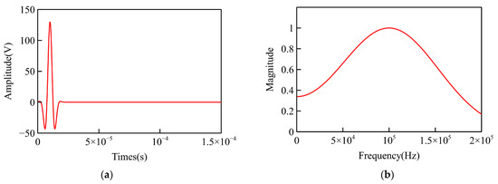
Figure 3.
The excitation signal: (a) Time-domain signal; (b) Frequency-domain signal.
3.2. The Finite Element Model
The methods for simulating the interaction between concrete defects and guided waves include the finite element method, the finite difference method, the boundary element method, and the spectral element method. Two integration schemes are generally used for the finite element problem of transient wave propagation: implicit FEM and explicit FEM (EFEM). The implicit integration method is unconditionally stable, but it takes longer to calculate each time increment; the explicit integration method has higher requirements for the time step, but the implicit integration method can be selected based on the specific calculation case. However, for wave propagation problems, the EFEM method is more widely used [34].
The numerical simulation process for time reversal focusing imaging using ABAQUS software can be divided into three stages: the preprocessing stage, the solution calculation stage, and the postprocessing stage. In the preprocessing stage, ABAQUS software was used to establish a homogeneous two-dimensional concrete model. The density of concrete was 2300 kg/m3, the Poisson’s ratio of concrete was 0.27, and the Young’s modulus of concrete was 26,000 MPa. The size of the model was 820 mm × 300 mm, and the sizes of the damages and the locations of the centers of the damages are shown in Figure 4. The first kind of damage was expressed as D1, the radius was 10 mm, and the coordinates of the damage center were (360, 100). The other forms of damage were represented in a similar way.
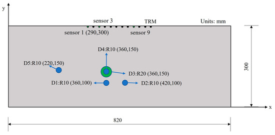
Figure 4.
FE model of concrete with hole damage.
The size of the largest finite element must be small enough to ensure the convergence of the calculation, and the smallest wavelength of the wave propagation can be identified [35]. Each wavelength must pass through at least 5–10 elements, and the time step must be determined based on the explicit and implicit integration methods and the excitation frequency [36], which satisfies , where c represents the wave speed. The propagation velocity of the longitudinal waves in this study is shown in Equation (11), where represents the Poisson’s ratio of concrete, and represents the density of concrete. Therefore, the CPS4R element, with a length of 1 mm, was chosen for this study. The wave propagation simulation used an explicit integration scheme with a time step of 5 × 10⁻⁹ s.
The output of the ABAQUS software included two parts: historical output data and field output data. The field output data mainly described the wave propagation process, while the historical output data were used to draw the transducer response curve. A linear sensor was placed on the concrete model, with the rectangular element serving as both the excitation point and the receiving point. The relative displacement of the polarization cross section of piezoelectric ceramics is proportional to the voltage amplitude. When an external stress and constraint are applied to the piezoelectric ceramic, the external stress is proportional to the voltage amplitude. Therefore, the piezoelectric smart aggregate model was omitted, and the corresponding point signal was used in the numerical simulation [37]. The distance between the excitation unit and the first receiving unit was 20 mm, which was used to simulate the excitation and reception of the concrete model due to the transducer. In total, 12 receiving units were spaced 20 mm apart, and the locations of sensor 1 were (290, 300), as shown in Figure 4. The load direction of the excitation unit was the same as the incident direction of the ultrasonic wave, and the change in magnitude was equal to the amplitude of the excitation signal waveform. The displacement variables in the y-axis direction of the receiving point were extracted as the historical output.
The time reversal focusing imaging result was related to the number of ABAQUS field outputs. To verify the computational stability of the finite element model, different field output numbers were used. The position of the focusing index, which was calculated by Equation (8), was extracted and compared with the actual damage position, as shown in Figure 5. The most accurate number of field outputs was calculated to be 500. When field outputs of 50 and 1000 were used, the results were the same and were more accurate than when field outputs of 300 and 800 were used. Although 500 was the most accurate field output number, when considering the calculation efficiency, 50 was relatively accurate. Therefore, the number of field outputs selected in this study was 50.
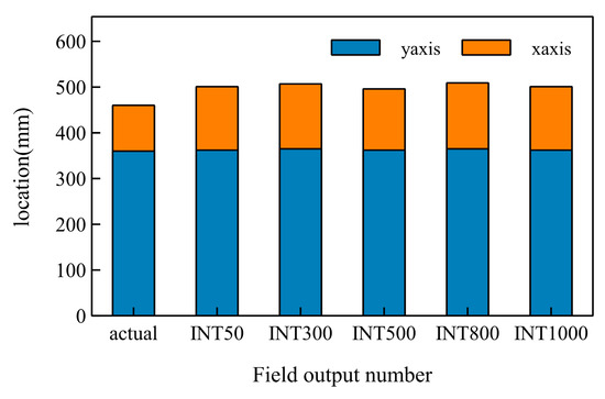
Figure 5.
The influence of the field output number on the imaging algorithm.
4. Results and Discussions
4.1. Forward Detection
Figure 6a,b show the damage signals and reference signals received by two receiving sensors (the third and ninth sensors). The damage signal was composed of the Rayleigh wave reflected by the boundary and the damage scattering signal. Compared with the amplitude of the Rayleigh wave reflected by the boundary, the amplitude of the damage scattering signal was much smaller. By comparing Figure 6a,b, the waveform of the damage signal received by the two sensors differed only in the time shift of the waveform. This result is consistent with the solution of the structural dynamics wave equation shown in Equation (3), which verifies the correctness of the numerical simulation.
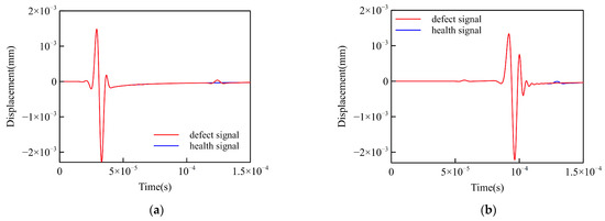
Figure 6.
Displacement signals of the damaged samples and baseline samples received at different points: (a) Signals received by sensor 3; (b) Signals received by sensor 9.
To analyze the damage signal and obtain damage-related information, the damage scattering signal based on the reference signal must be determined. The maximum amplitudes of the damage signal and the damage scattering signal are shown in Figure 6. In the five damage cases, the maximum amplitude of the damage signal received by each sensor was connected by a curve and normalized, as shown in Figure 6a. Furthermore, the maximum amplitude of the damage scattering signal received by each sensor was connected by a curve and normalized, as shown in Figure 6b.
Figure 7a shows that the trend of the damage signal essentially coincides with each damage form. In contrast, as shown in Figure 7b, the maximum value of the D1 curve occurred between the fourth and sixth sensors, while the maximum value of the D2 curve occurred between the 6th and 8th sensors, corresponding to D1 and D2 in Figure 4, respectively. The maximum values of the D3 and D4 curves occurred between the seventh and ninth sensors, which does not match the actual status. The damage may have been too close to the sensor array. According to the findings in [38], when the observation point is too close to the excitation source, it is easily affected by the near field of the excitation source. When the receiving point is too close to the damage, it receives both the clutter reflected by the damage and the transmitted wave. The trend of the fifth damage curve was completely opposite to the trends of the other four cases, possibly because the fifth type of damage was completely outside the range of the sensor. This result shows that the effectiveness of nondestructive concrete evaluation depends on the relative position of the sensor array and the damage [39].
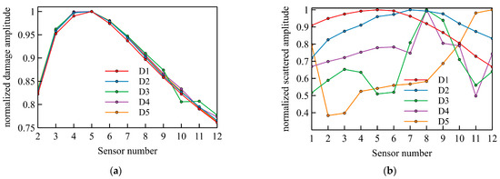
Figure 7.
Maximum amplitudes of the received signal at the time reversal mirror for five types of damage: (a) Damage signal; (b) Damage scattering signal.
Because the first and second damage scattering signals contain more damage information, as described in the previous section, the time profile of the damage scattering signal is plotted in Figure 8. Figure 8a,b show the time profiles of the damage scattering signal for two damage cases (D1 and D2). The time profile was based on the location of the sensor, the damage scattering signal, and the signal propagation time [40]. Based on the two circled positions in Figure 8, the location of the damage can be roughly estimated. The first damage is located between (350, 375), while the second damage is located between (400, 425). This conclusion is consistent with Figure 8. The time profile of the damage scattering signal can be used to predict the location of the damage by determining the time of flight (TOF) between the signal and the echo; in addition, the distance between the damage and the transducer can be determined [41]. When the distance between the damage and the TRM varies, as the distance between the sensor and the damage decreases; the time at which the damage scattering signal arrives also decreases.
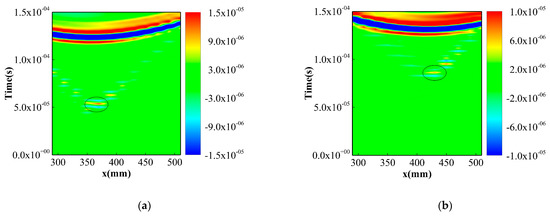
Figure 8.
Time profiles of the damage scattering signal: (a) Damage 1; (b) Damage 2.
Although the forward algorithm is not computationally intensive and is simple to implement, it can only determine the approximate location of the damage or evaluate the severity of the damage [42,43]. In contrast, time reversal focusing uses information from both the forward field and the reverse field, which improves the imaging ability. Moreover, time reversal focusing depends on damage information in the signal [44]. In Figure 8, the amplitude of the scattered wave due to damage was much smaller than the amplitude of the direct wave; in Figure 8, the scattering signals caused by the various types of damage were quite different, indicating that this signal contained more damage information. Mori [28] reversed the damage scattering signal and damage signal, compared the imaging ability based on the damage scattering field and the total field, and found that imaging based on the damage scattering field was superior to imaging based on the total field. Therefore, the imaging algorithm used in Section 4.2 of this study was based on time reversal focusing of the damage scattering field, and the effect of time focusing on spatial focusing was analyzed.
4.2. Time Reversal Focusing Imaging
The damage imaging shown in Figure 9a is composed of the maximum value of all imaging points in the propagation time, with spatial focusing information and no time focusing information. Figure 9b shows the damage imaging formed by the focusing index corresponding to the time, which contains time focusing information and satisfies both time focusing and spatial focusing. Figure 9a has more artifacts; only the general direction of the damage is known, and the damage cannot be effectively located. Although there are artifacts in the boundary area of Figure 9b, the damage location is clear and accurate, and the imaging ability is greatly improved. Comparing Figure 9a,b shows that time focusing clearly improved spatial focusing. Douma [45] reached similar conclusions in a geological imaging study. When the time reversal method is used for imaging, it mainly depends on the ability of the measured scattering waveform to be compressed to a point in time and space [41].
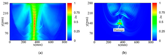
Figure 9.
Time reversal focusing imaging: (a) Unsatisfactory time focusing; (b) Satisfactory time focusing.
Taking the focusing index point as a reference, the focusing indices of the imaging points parallel to the x-axis and y-axis were extracted, and the relationship between the imaging area and the focusing index is shown in Figure 10b,c. The focusing curve along the y-axis, shown in Figure 10b, has two spectral peaks, located at the main lobe and the side lobe. The distance between these two points with a normalized focusing index of 0.5 was defined as the main lobe width [46], which is used to characterize the spatial focusing properties. This value is called the spatial resolution. A side lobe with a normalized focusing index of 0.4 was also located near the main lobe. The curve in the x-axis direction is shown in Figure 10c. Because the array sensor was not arranged in the y-axis direction, the focusing curve contained only the main lobe, which characterized the focusing quality, with no side lobes.
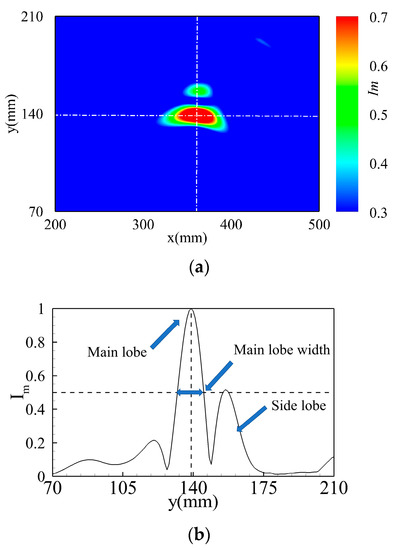
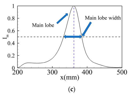
Figure 10.
The focusing ability of the time reversal focusing algorithm: (a) Time reversal focusing imaging satisfies time focusing; (b) The focusing curve in the y-axis direction; (c) The focusing curve in the x-axis direction.
4.3. Time Reversal Focusing Curve
Figure 11, Figure 12 and Figure 13 plot the focusing curves of the different damage forms to evaluate the relationship between the different forms and their time reversal focusing abilities. Unless otherwise specified, the following focusing curve refers to the normalized focusing curve. For the first, third, and fourth types of damage (D1, D3, and D4), the x-axis coordinates were the same, the positions of the third and fourth damages were coincident, and the diameter of D3 was the largest. The focusing curves for these three types of damage are plotted in Figure 11. Figure 11a shows the focusing curves along the y-axis. D3 and D4 were from D1, which is reasonable. Figure 11b shows the focusing curves along the x-axis. The x-coordinate of these three types of damage was 361, which was close to the actual damage coordinate of 360. This result illustrates the feasibility of using the focusing curve to determine the location of the damage. In addition, unlike Mori’s [28] research, the focusing curves shown in Figure 11b only have a main lobe. As the sensors in Mori’s research were arranged around the damage, the focusing curves along the x- and y-axes had both a main lobe and a side lobe.
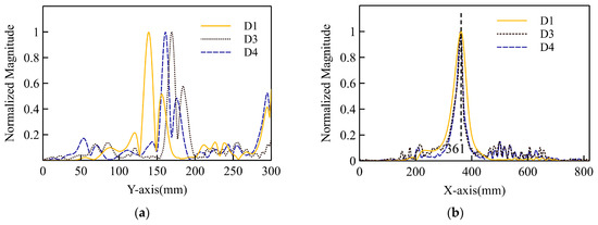
Figure 11.
The focusing curves of the first, third, and fourth types of damage: (a) Y-direction; (b) X-direction.
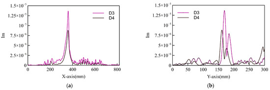
Figure 12.
The stress focusing curves of the third and fourth types of damage: (a) X-direction; (b) Y-direction.
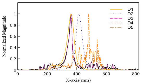
Figure 13.
X-direction focusing curves of the five types of damage.
The stress focusing curves of D3 and D4 were plotted to further illustrate the role of the time reversal focusing curve in identifying damage. Figure 12 shows the stress focusing curves of the third and fourth types of damage along the x- and y-axes. Figure 12a shows the focusing curves along the x-axis. The two focusing curves nearly overlap, with the third type of damage having a larger amplitude. The third type of damage had a slightly higher spatial resolution than the fourth type of damage. Figure 12b shows the focusing curves along the y-axis, which were similar to the focusing curves along the x-axis, with the third type of damage having a larger amplitude. This result shows that the focusing curve can determine the position and size of the damage. Furthermore, the positioning effect in the x-axis direction is better than that in the y-axis direction based on the location of the main lobe in Figure 12a,b. The reason for this result is that the sensors were placed on one side of the damage rather than arranged around the damage, demonstrating the effect of sensor placement on time reversal focusing.
Because the curve focusing on the x-axis direction better reflected the damage information, its imaging accuracy was higher. Figure 13 compares the x-axis direction-focusing curves of the different types of damage. D2 was located to the right of D1, which is realistic. The focusing curve of D5 had more lobes than the other four types of damage and the opposite positioning direction because D5 was outside the detection range of the sensor, as shown in Figure 4. The trend of the maximum value of the damage scattering signal received by the sensor array in D5 was opposite to that of the other four types of damage, as described in Section 4.1. The signal lacked damage-related information because of the relative position of the sensor and the damage [47]. In addition, Qiu [48,49] showed that a good focusing effect in time reversal focusing imaging is directly related to the phase. However, whether the damage is arranged in the sensor pair or not affects the phase change but not the amplitude. Therefore, the focusing curve of D5 cannot adequately represent the damage.
Based on the above discussion, the damage imaging map can visualize and directly display the damage, but it cannot provide the exact imaging resolution. By extracting the focusing curve of the damage, the resolution can be calculated, and the damage information can be interpreted in more detail. In addition, the concrete model in this paper does not consider the effect of aggregates and is still a preliminary model for studying imaging algorithm resolution and structural damage identification. To avoid the negative effects of damage and reduce maintenance costs, in addition to the cybernetic engineering method of self-healing [50], embedded piezoelectric sensors can also be studied. The construction period can be quickly and safely shortened by monitoring the hydration process of concrete structures based on embedded piezoelectric sensors [51].
Although embedded piezoelectric sensors can realize real-time detection of newly built concrete structures, the energy of the compression waves (P waves) generated by embedded sensors is insufficient at present. P waves have been used to monitor crack initiation in reinforced concrete beams online. To excite the waves, 800 volts of electricity are needed, which indicates that the use of P waves in crack detection is still limited [52]. The method proposed in this paper depends on damage information in the damage scattering signals. Considering the influence of steel bars on damage scattering signals, this method can also be applied to reinforced concrete by using surface waves and proper signal processing, which means it may depend on the strength of the excitation signal and the signal processing technology. Therefore, in future work, the effectiveness of the algorithm needs to be verified by using embedded piezoelectric sensors and reinforced concrete beams. Nevertheless, the results in this paper support the application of the time reversal focusing algorithm to concrete and can be used as a reference for future concrete damage imaging research.
5. Conclusions
In this study, pulse-echo time reversal imaging, which is based on the time reversal focus imaging algorithm and operates in pulse-echo mode on a sensor array, was realized. The proposed algorithm was verified with five different damage forms, and the x-axis and y-axis focusing curves of each type of damage were obtained. Based on the overall results and analyses, the following conclusions can be drawn:
- The damage signals received by sensors 3 and 9 only exhibit a time shift in the signal waveform, which is consistent with the structural dynamics, indicating the correctness of the numerical model.
- A comparison of the time profiles of the damage scattering signal and the time reversal focusing imaging showed the superiority of the reversal algorithm. Time reversal focusing uses information from both the forward field and the reverse field, thereby improving the imaging ability.
- An improved time reversal focusing imaging algorithm that also satisfies time focusing was used to investigate the effect of time focusing on spatial focusing. This work can serve as a reference for future concrete damage imaging research.
- The maximum value of the D3 focusing curve was significantly higher than that of the D4 focusing curve. The location of the main lobe was in good agreement with the actual location of the damage, indicating that the location and size of the damage can be determined based on the focusing curve.
Author Contributions
Conceptualization, X.S. and S.F.; software, X.S.; validation, S.F., X.S. and C.L.; investigation, X.S.; data curation, X.S.; writing—original draft preparation, X.S.; writing—review and editing, S.F., X.S. and C.L. All authors have read and agreed to the published version of the manuscript.
Funding
This research was funded by the Scientific Research Fund of Institute of Engineering Mechanics China Earthquake Administration (Grant No. 2020D31), the Funds for International Cooperation and Exchange of the National Natural Science Foundation of China (Grant No. 52020105005), and the Natural Science Foundation of China (Grant No. 51978507).
Data Availability Statement
Not applicable.
Conflicts of Interest
The authors declare no conflict of interest.
References
- Meola, C.; Carlomagno, G.M. Recent Advances in the Use of Infrared Thermography. Meas. Sci. Technol. 2004, 15, R27–R58. [Google Scholar] [CrossRef]
- Santos, V.R.N.; Teixeira, F.L. Study of time-reversal-based signal processing applied to polarimetric GPR detection of elongated targets. J. Appl. Geophys. 2017, 139, 257–268. [Google Scholar] [CrossRef]
- Mohan, A.; Poobal, S. Crack Detection Using Image Processing: A Critical Review and Analysis. Alex. Eng. J. 2018, 57, 787–798. [Google Scholar] [CrossRef]
- Yu, H.; Lu, L.; Qiao, P. Localization and Size Quantification of Surface Crack of Concrete Based on Rayleigh Wave Attenuation Model. Constr. Build. Mater. 2021, 280, 122437. [Google Scholar] [CrossRef]
- Han, H.; Deng, H.; Dong, Q.; Gu, X.; Zhang, T.; Wang, Y. An Advanced Otsu Method Integrated with Edge Detection and Decision Tree for Crack Detection in Highway Transportation Infrastructure. Adv. Mater. Sci. Eng. 2021, 2021, 9205509. [Google Scholar] [CrossRef]
- Carrasco, M.; Araya-Letelier, G.; Velazquez, R.; Visconti, P. Image-Based Automated Width Measurement of Surface Cracking. Sensors 2021, 21, 7534. [Google Scholar] [CrossRef]
- Yu, H.; Lu, L.; Qiao, P.; Wang, Z. Actuating and Sensing Mechanism of Embedded Piezoelectric Transducers in Concrete. Smart Mater. Struct. 2020, 29, 085020. [Google Scholar] [CrossRef]
- Tang, Z.S.; Lim, Y.Y.; Smith, S.T.; Izadgoshasb, I. Development of analytical and numerical models for predicting the mechanical properties of structural adhesives under curing using the PZT-based wave propagation technique. Mech. Syst. Signal Proc. 2019, 128, 172–190. [Google Scholar] [CrossRef]
- Zima, B. Damage Detection in Plates Based on Lamb Wavefront Shape Reconstruction. Measurement 2021, 177, 109206. [Google Scholar] [CrossRef]
- Zaki, A.; Chai, H.K.; Aggelis, D.G.; Alver, N. Non-Destructive Evaluation for Corrosion Monitoring in Concrete: A Review and Capability of Acoustic Emission Technique. Sensors 2015, 15, 19069–19101. [Google Scholar] [CrossRef]
- Qing, X.; Li, W.; Wang, Y.; Sun, H. Piezoelectric Transducer-Based Structural Health Monitoring for Aircraft Applications. Sensors 2019, 19, 545. [Google Scholar] [CrossRef] [PubMed]
- Choi, H.; Popovics, J.S. NDE Application of Ultrasonic Tomography to a Full-Scale Concrete Structure. IEEE Trans. Ultrason. Ferroelectr. Freq. Control 2015, 62, 1076–1085. [Google Scholar] [CrossRef] [PubMed]
- Kwon, H.; Joh, C.; Chin, W.J. 3D Internal Visualization of Concrete Structure Using Multifaceted Data for Ultrasonic Array Pulse-Echo Tomography. Sensors 2021, 21, 6681. [Google Scholar] [CrossRef] [PubMed]
- Kwon, H.; Joh, C.; Chin, W.J. Pulse Peak Delay-Total Focusing Method for Ultrasonic Tomography on Concrete Structure. Appl. Sci. 2021, 11, 1741. [Google Scholar] [CrossRef]
- Zielińska, M.; Rucka, M. Detection of Debonding in Reinforced Concrete Beams Using Ultrasonic Transmission Tomography and Hybrid Ray Tracing Technique. Constr. Build. Mater. 2020, 262, 120104. [Google Scholar] [CrossRef]
- Ganguli, A.; Rappaport, C.M.; Abramo, D.; Wadia-Fascetti, S. Synthetic Aperture Imaging for Flaw Detection in a Concrete Medium. NDT E Int. 2012, 45, 79–90. [Google Scholar] [CrossRef]
- Gao, W.; Huo, L.; Li, H.; Song, G. Smart Concrete Slabs with Embedded Tubular PZT Transducers for Damage Detection. Smart Mater. Struct. 2018, 27, 025002. [Google Scholar] [CrossRef]
- Gao, W.; Huo, L.; Li, H.; Song, G. An Embedded Tubular PZT Transducer Based Damage Imaging Method for Two-Dimensional Concrete Structures. IEEE Access 2018, 6, 30100–30109. [Google Scholar] [CrossRef]
- Alleyne, D.N.; Pavlakovic, B.; Lowe, M.J.S.; Cawley, P. Rapid, Long Range Inspection of Chemical Plant Pipework Using Guided Waves. AIP Conf. Proc. 2001, 557, 180–187. [Google Scholar] [CrossRef]
- Huo, H.; He, J.; Guan, X. A Bayesian Fusion Method for Composite Damage Identification Using Lamb Wave. Struct. Health Monit. 2020, 147592172094500. [Google Scholar] [CrossRef]
- Kozlov, A.V.; Kozlov, V.N. The Development and Current State of Methods for the Nondestructive Testing and Acoustic Tomography of Concrete. Russ. J. Nondestruct. Test. 2015, 51, 329–337. [Google Scholar] [CrossRef]
- Zhao, G.; Zhang, D.; Zhang, L.; Wang, B. Detection of Defects in Reinforced Concrete Structures Using Ultrasonic Nondestructive Evaluation with Piezoceramic Transducers and the Time Reversal Method. Sensors 2018, 18, 4176. [Google Scholar] [CrossRef] [PubMed] [Green Version]
- Fink, M.; Prada, C.; Wu, F.; Cassereau, D. Self Focusing in Inhomogeneous Media with Time Reversal Acoustic Mirrors. In Proceedings of the IEEE Ultrasonics Symposium, Montreal, QC, Canada, 3–6 October 1989; Volume 2, pp. 681–686. [Google Scholar]
- Liang, J.; Chen, B.; Shao, C.; Li, J.; Wu, B. Time Reverse Modeling of Damage Detection in Underwater Concrete Beams Using Piezoelectric Intelligent Modules. Sensors 2020, 20, 7318. [Google Scholar] [CrossRef] [PubMed]
- Prada, C.; Manneville, S.; Spoliansky, D.; Fink, M. Decomposition of the Time Reversal Operator: Detection and Selective Focusing on Two Scatterers. J. Acoust. Soc. Am. 1996, 99, 2067–2076. [Google Scholar] [CrossRef]
- Becht, P.; Deckers, E.; Claeys, C.; Pluymers, B.; Desmet, W. Loose Bolt Detection in a Complex Assembly Using a Vibro-Acoustic Sensor Array. Mech. Syst. Signal Process. 2019, 130, 433–451. [Google Scholar] [CrossRef]
- Wang, J.; Shen, Y. An enhanced Lamb wave virtual time reversal technique for damage detection with transducer transfer function compensation. Smart Mater. Struct. 2019, 28, 085017. [Google Scholar] [CrossRef]
- Mori, N.; Biwa, S.; Kusaka, T. Damage Localization Method for Plates Based on the Time Reversal of the Mode-Converted Lamb Waves. Ultrasonics 2019, 91, 19–29. [Google Scholar] [CrossRef]
- Jonsson, B.L.G.; de Hoop, M.V.; Gustafsson, M.; Weston, V.H. Retrofocusing of Acoustic Wave Fields by Iterated Time Reversal. SIAM J. Appl. Math. 2004, 64, 1954–1986. [Google Scholar] [CrossRef] [Green Version]
- Wang, S.; Wu, W.; Shen, Y.; Liu, Y.; Jiang, S. Influence of the PZT Sensor Array Configuration on Lamb Wave Tomography Imaging with the RAPID Algorithm for Hole and Crack Detection. Sensors 2020, 20, 860. [Google Scholar] [CrossRef] [Green Version]
- Borcea, L.; Papanicolaou, G.; Tsogka, C. Imaging and Time Reversal in Random Media. Inverse Probl. 2002, 18, 1247–1279. [Google Scholar] [CrossRef] [Green Version]
- Mukherjee, S.; Mays, R.O.; Tringe, J.W. A Microwave Time Reversal Algorithm for Imaging Extended Defects in Dielectric Composites. IEEE Trans. Comput. Imaging 2021, 7, 1215–1227. [Google Scholar] [CrossRef]
- Abbas, M.; Shafiee, M. Structural Health Monitoring (SHM) and Determination of Surface Defects in Large Metallic Structures using Ultrasonic Guided Waves. Sensors 2018, 18, 3958. [Google Scholar] [CrossRef] [PubMed] [Green Version]
- Stojic, D.; Nestorovic, T.; Markovic, N.; Marjanovic, M. Experimental and Numerical Research on Damage Localization in Plate-Like Concrete Structures Using Hybrid Approach. Struct. Control Health Monit. 2018, 25, e2214. [Google Scholar] [CrossRef]
- Ghavamian, A.; Mustapha, F.; Baharudin, B.T.H.T.; Yidris, N. Detection, Localisation and Assessment of Defects in Pipes Using Guided Wave Techniques: A Review. Sensors 2018, 18, 4470. [Google Scholar] [CrossRef] [Green Version]
- Mitra, M.; Gopalakrishnan, S. Guided wave based structural health monitoring: A review. Smart Mater. Struct. 2016, 25, 053001. [Google Scholar] [CrossRef]
- Zheng, J. Research on Health Monitoring and Numerical Simulation of Concrete Structures Based on Smart Materials. Master’s Thesis, Changsha University of Science Technology, Changsha, China, 2018. [Google Scholar]
- Ou, Y. Numerical Analysis of Material Surface Defect Depth Detection Using Rayleigh Wave. Master’s Thesis, Harbin Institute of Technology, Harbin, China, 2014. [Google Scholar]
- Thiene, M.; Khodaei, Z.S.; Aliabadi, M.H. Optimal Sensor Placement for Maximum Area Coverage (MAC) for Damage Localization in Composite Structures. Smart Mater. Struct. 2016, 25, 095037. [Google Scholar] [CrossRef]
- Yan, G.; Zhou, L. Real time identification of damages for plate-like structure using migration technique in frequency-wavenumber domain. J. Vib. Eng. 2008, 21, 620–625. [Google Scholar] [CrossRef]
- Monaco, E.; Ricci, F.; Lecce, L.; Boffa, N.D. Application of the Beam-Forming Technique for Damage Detection in Composite Plate. In Proceedings of the ASME 2012 Noise Control and Acoustics Division Conference at InterNoise 2012, New York, NY, USA, 19–22 August 2012. [Google Scholar]
- Mustapha, S.; Ye, L.; Wang, D.; Lu, Y. Assessment of Debonding in Sandwich CF/EP Composite Beams Using A0 Lamb Wave at Low Frequency. Compos. Struct. 2011, 93, 483–491. [Google Scholar] [CrossRef]
- Gao, F.; Zeng, L.; Lin, J.; Shao, Y. Damage Assessment in Composite Laminates via Broadband Lamb Wave. Ultrasonics 2018, 86, 49–58. [Google Scholar] [CrossRef]
- Anderson, B.E.; Douma, J.; Ulrich, T.J.; Snieder, R. Improving Spatio-Temporal Focusing and Source Reconstruction Through Deconvolution. Wave Motion 2015, 52, 151–159. [Google Scholar] [CrossRef] [Green Version]
- Douma, J.; Niederleithinger, E.; Snieder, R. Locating Events Using Time Reversal and Deconvolution: Experimental Application and Analysis. J. Nondestruct. Eval. 2015, 34, 2. [Google Scholar] [CrossRef]
- Park, H.W. Numerical Simulation and Investigation of the Spatial Focusing of Time Reversal A0 Lamb Wave Mode Using Circular Piezoelectric Transducers Collocated on a Rectangular Plate. J. Sound Vib. 2013, 332, 2672–2687. [Google Scholar] [CrossRef]
- Kocherla, A.; Kolluru, S.V.L. Embedded smart PZT-based sensor for internal damage detection in concrete under applied compression. Measurement 2020, 163, 108018. [Google Scholar] [CrossRef]
- Qiu, L.; Yuan, S.; Su, Y.; Zhang, X. Multiple Impact Source Imaging and Localization on Composite Structure Based on Shannon Complex Wavelet and Time Reversal Focusing. Acta Aeronaut. Astronaut. Sin. 2010, 31, 2417–2424. [Google Scholar]
- Qiu, L.; Yuan, S.; Zhang, X.; Wang, Y. A Time Reversal Focusing Based Impact Imaging Method and Its Evaluation on Complex Composite Structures. Smart Mater. Struct. 2011, 20, 105014. [Google Scholar] [CrossRef]
- Insaurralde, C.C.; Rahman, P.K.S.M.; Ramegowda, M.; Vemury, C.M. Follow-up Methods for Autonomic Repairing Process Cybernetic Concrete for Civil Self-healing Structures. In Proceedings of the 2016 IEEE International Conference on Systems, Man, and Cybernetics (SMC), Budapest, Hungary, 9–12 October 2016; IEEE: New York, NY, USA, 2016; pp. 4854–4859. [Google Scholar]
- Karaiskos, G.; Deraemaeker, A.; Aggelis, D.G.; Van Hemelrijck, D. Monitoring of concrete structures using the ultrasonic pulse velocity method. Smart Mater. Struct. 2015, 24, 113001. [Google Scholar] [CrossRef] [Green Version]
- Dumoulin, C.; Karaiskos, G.; Sener, J.-Y.; Deraemaeker, A. Online monitoring of cracking in concrete structures using embedded piezoelectric transducers. Smart Mater. Struct. 2014, 23, 115016. [Google Scholar] [CrossRef]
Publisher’s Note: MDPI stays neutral with regard to jurisdictional claims in published maps and institutional affiliations. |
© 2022 by the authors. Licensee MDPI, Basel, Switzerland. This article is an open access article distributed under the terms and conditions of the Creative Commons Attribution (CC BY) license (https://creativecommons.org/licenses/by/4.0/).