
Revealing Microclimate around Buildings with Long-Term Monitoring through the Neural Network Algorithms


Abstract
:1. Introduction
2. Methodology
2.1. Overview of the Methodology
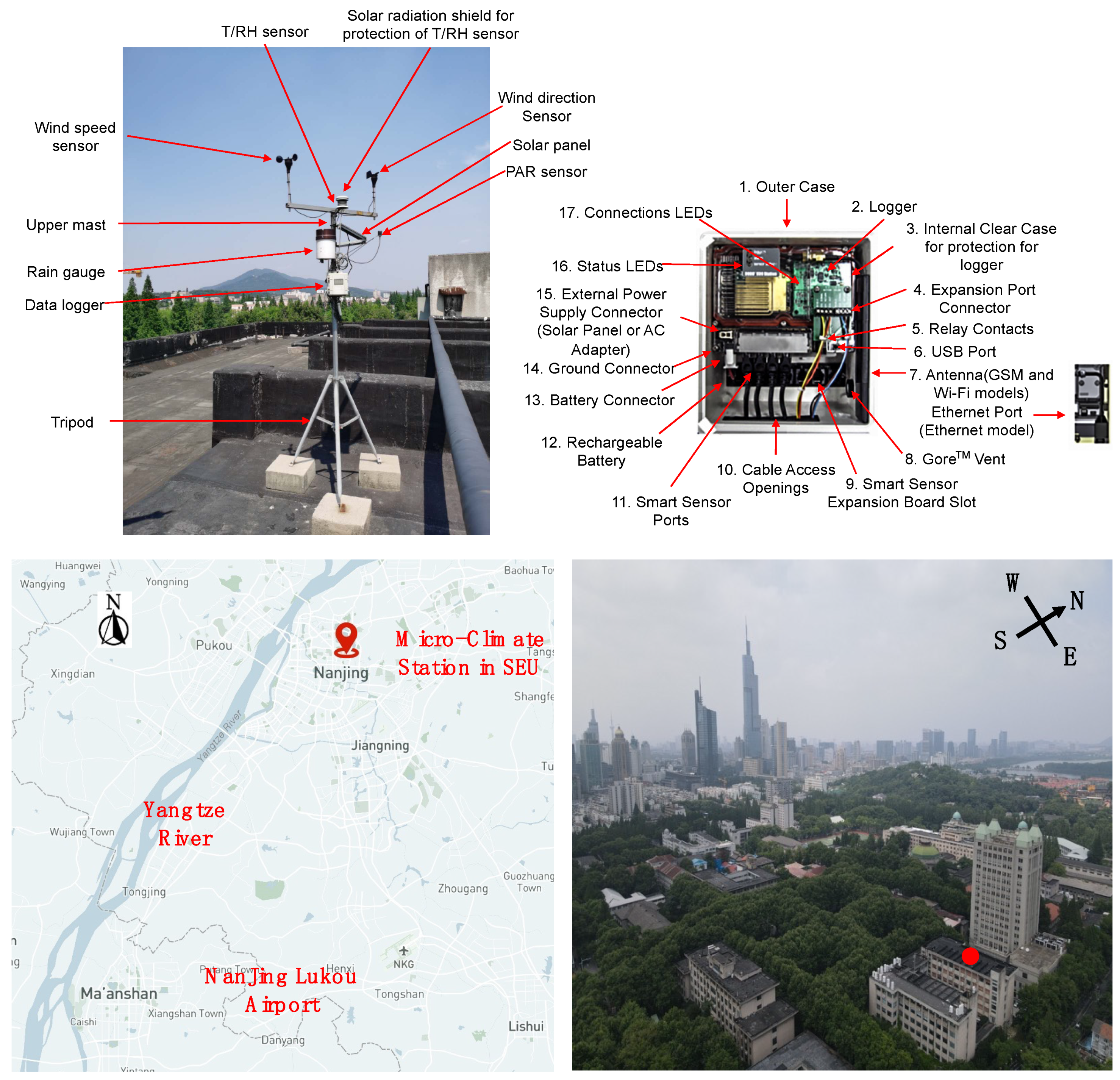
2.2. Case Experiment of Urban Microclimate Monitoring
2.3. Data Pre-Processing
2.4. Predictive Techniques in This Study
2.4.1. BP-ANN Predictive Technique
2.4.2. LSTM Predictive Technique
2.5. Model Tunning of Two Predictive Techniques
3. Results
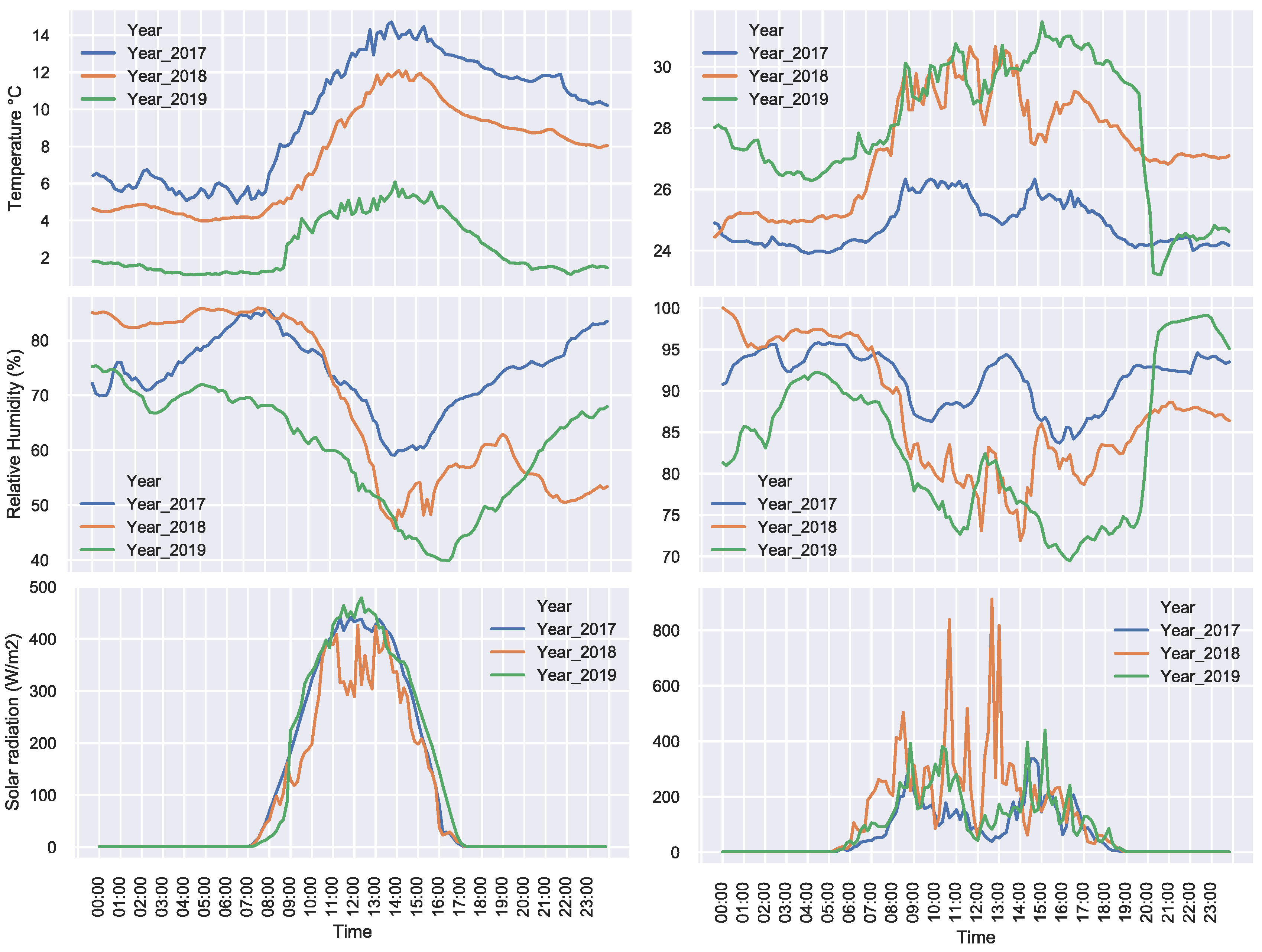
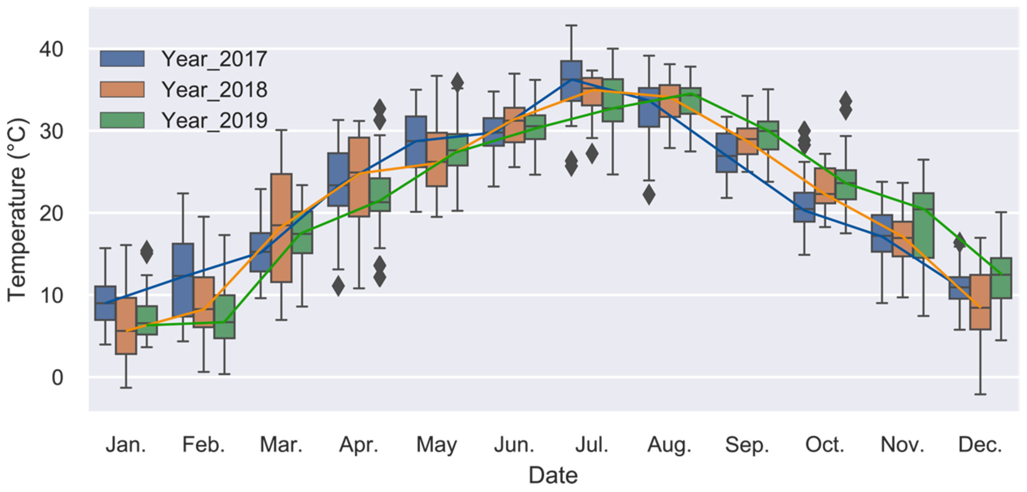
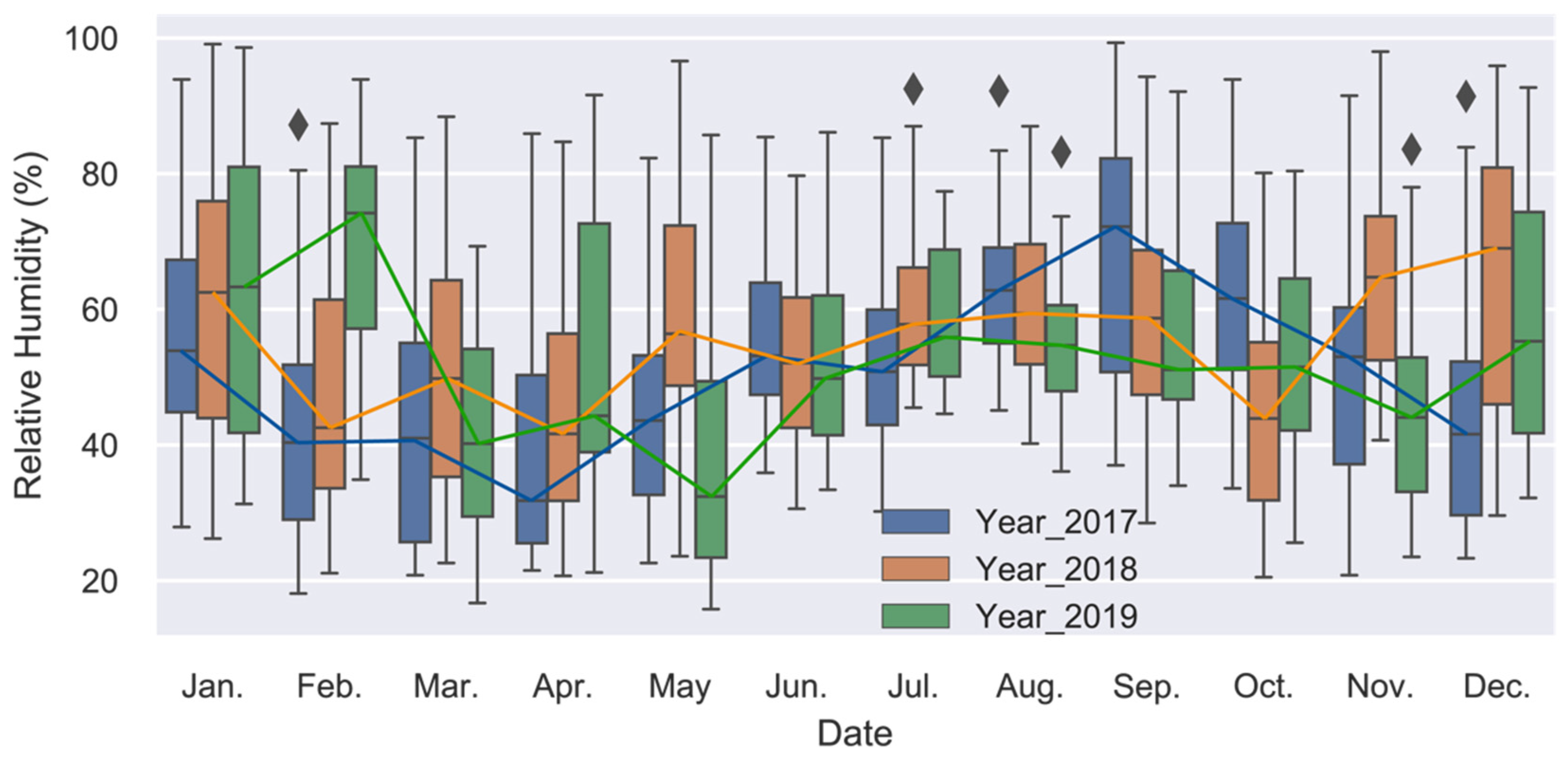
3.1. Results of Long-Term Microclimate Monitoring
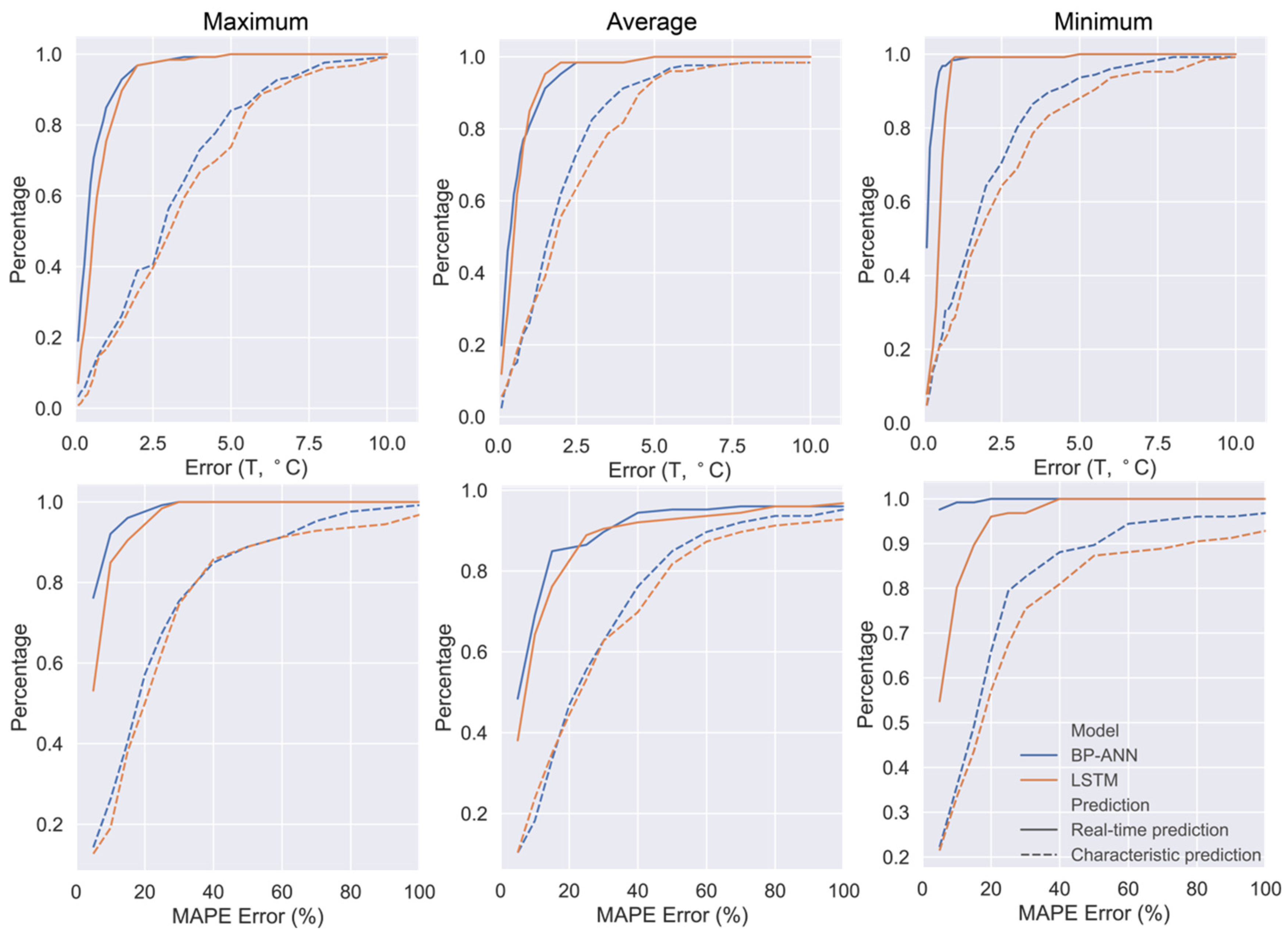
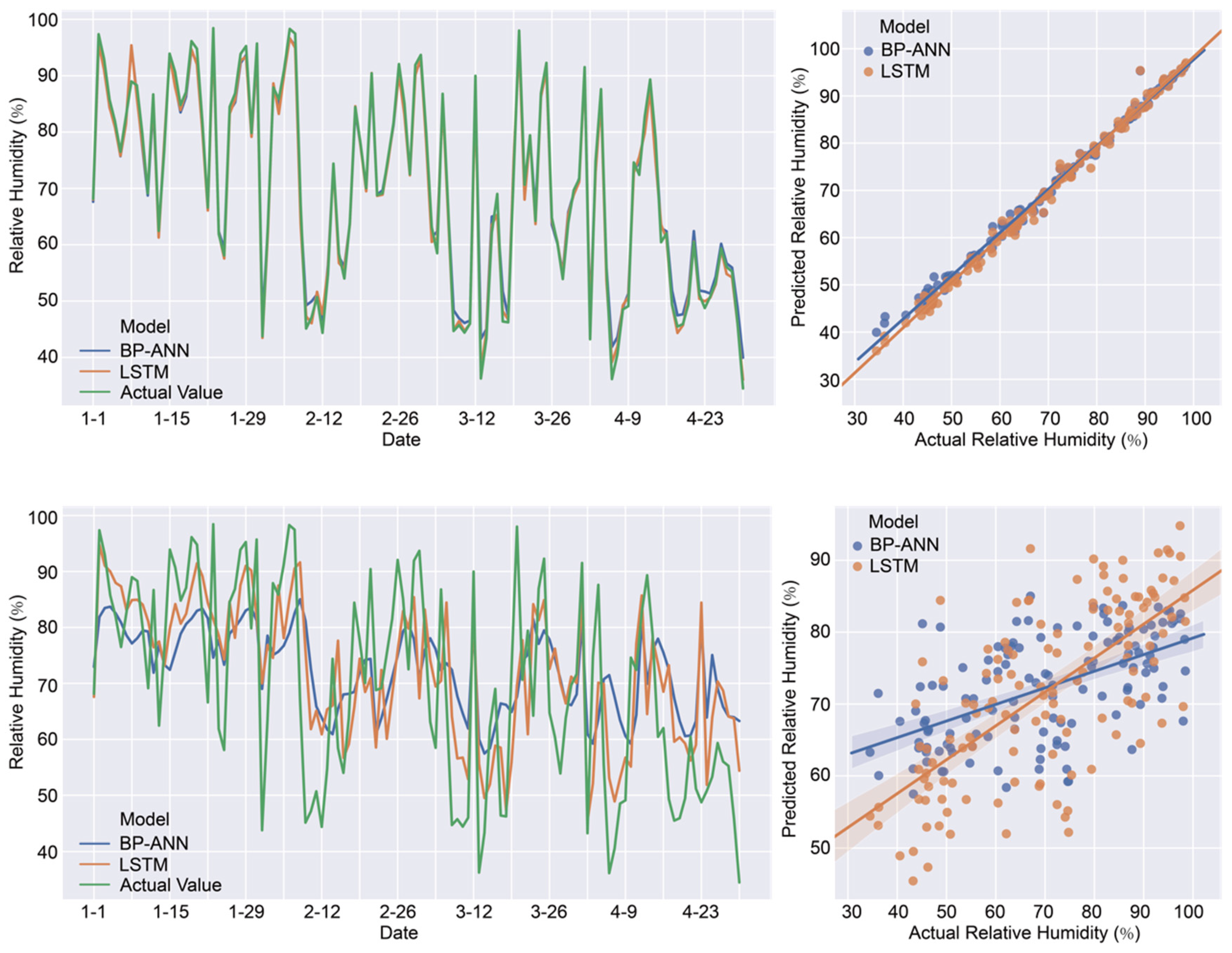
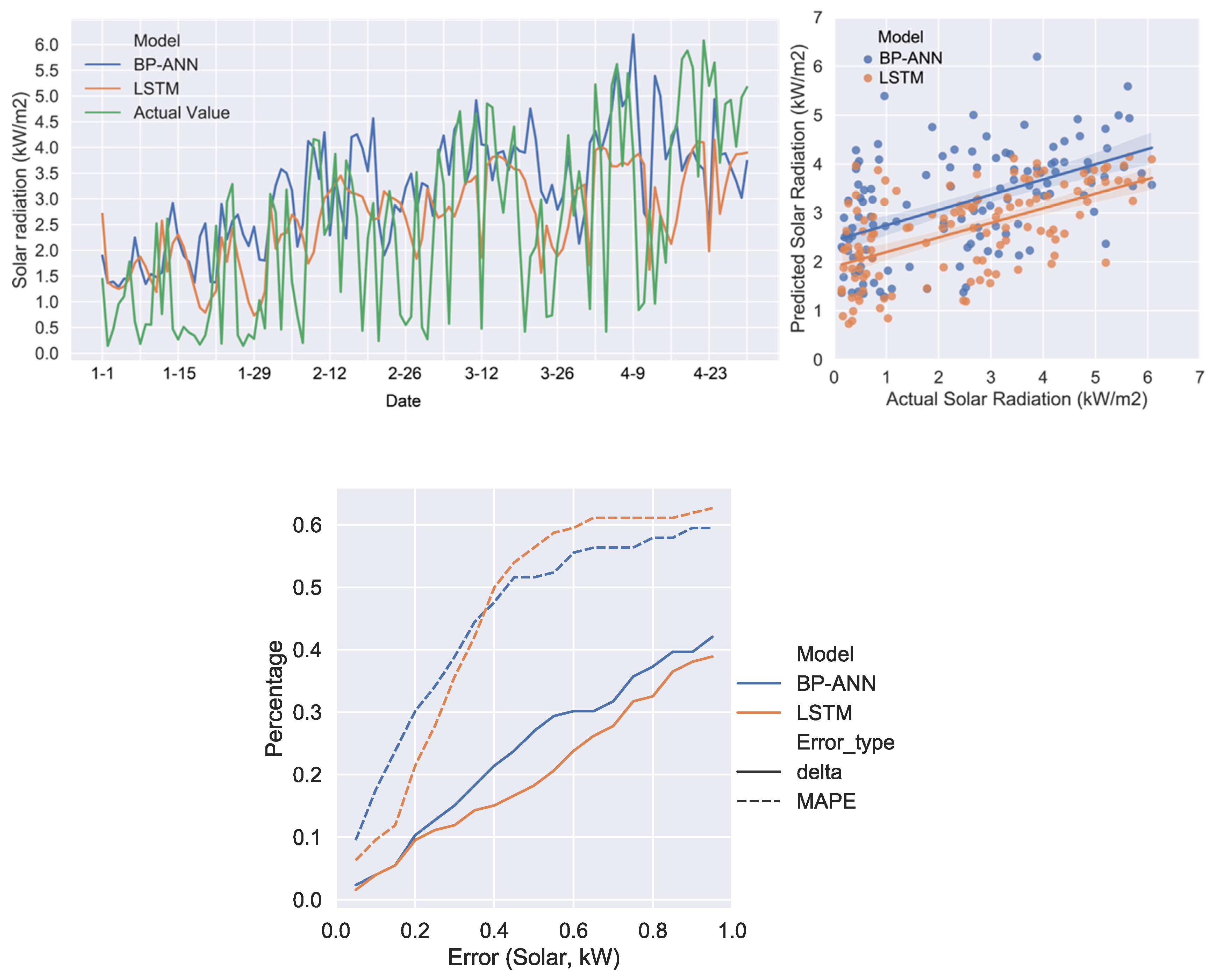
3.2. Results of Predictive Models
4. Discussion
5. Conclusions
Author Contributions
Funding
Data Availability Statement
Conflicts of Interest
Appendix A


References
- National Bureau of Statistics of China. China Statistical YearBook 2021; China Statistics Press: Beijing, China, 2021.
- Xu, X.; Wu, Y.; Wang, W.; Hong, T.; Xu, N. Performance-driven optimization of urban open space configuration in the cold-winter and hot-summer region of China. Build. Simul. 2019, 12, 411–424. [Google Scholar] [CrossRef] [Green Version]
- Elnabawi, M.H.; Hamza, N. Outdoor thermal comfort: Coupling microclimatic parameters with subjective thermal assessment to design urban performative spaces. Buildings 2020, 10, 238. [Google Scholar] [CrossRef]
- Javanroodi, K.; Nik, V.M. Impacts of microclimate conditions on the energy performance of buildings in urban areas. Buildings 2019, 9, 189. [Google Scholar] [CrossRef] [Green Version]
- Leroyer, S.; Bélair, S.; Spacek, L.; Gultepe, I. Modelling of radiation-based thermal stress indicators for urban numerical weather prediction. Urban Clim. 2018, 25, 64–81. [Google Scholar] [CrossRef]
- Othman, N.E.; Zaki, S.A.; Rijal, H.B.; Ahmad, N.H.; Razak, A.A. Field study of pedestrians’ comfort temperatures under outdoor and semi-outdoor conditions in Malaysian university campuses. Int. J. Biometeorol. 2021, 65, 453–477. [Google Scholar] [CrossRef]
- Hayles, C.; Huddleston, M.; Chinowsky, P.; Helman, J. Quantifying the Effects of Projected Climate Change on the Durability and Service Life of Housing in Wales, UK. Buildings 2022, 12, 184. [Google Scholar] [CrossRef]
- Zhao, Y.; Zang, Z.; Zhang, W.; Wei, S.; Xuan, Y. Predicting indoor temperature distribution based on contribution ratio of indoor climate (Cri) and mobile sensors. Buildings 2021, 11, 458. [Google Scholar] [CrossRef]
- Heidari, H.; Mohammadbeigi, A.; Khazaei, S.; Soltanzadeh, A.; Asgarian, A.; Saghafipour, A. The effects of climatic and environmental factors on heat-related illnesses: A systematic review from 2000 to 2020. Urban Clim. 2020, 34, 100720. [Google Scholar] [CrossRef]
- Sankar Cheela, V.R.; John, M.; Biswas, W.; Sarker, P. Combating urban heat island effect—a review of reflective pavements and tree shading strategies. Buildings 2021, 11, 93. [Google Scholar] [CrossRef]
- Alnusairat, S.; Ayyad, Y.; Al-Shatnawi, Z. Towards meaningful university space: Perceptions of the quality of open spaces for students. Buildings 2021, 11, 556. [Google Scholar] [CrossRef]
- Lai, D.; Chen, B.; Liu, K. Quantification of the influence of thermal comfort and life patterns on outdoor space activities. Build. Simul. 2020, 13, 113–125. [Google Scholar] [CrossRef]
- Zhang, C.; Liao, H.; Strobl, E.; Li, H.; Li, R.; Jensen, S.S.; Zhang, Y. The role of weather conditions in COVID-19 transmission: A study of a global panel of 1236 regions. J. Clean. Prod. 2021, 292, 125987. [Google Scholar] [CrossRef] [PubMed]
- Wang, W.; Li, S.; Guo, S.; Ma, M.; Feng, S.; Bao, L. Benchmarking urban local weather with long-term monitoring compared with weather datasets from climate station and EnergyPlus weather (EPW) data. Energy Rep. 2021, 7, 6501–6514. [Google Scholar] [CrossRef]
- Merlier, L.; Frayssinet, L.; Johannes, K.; Kuznik, F. On the impact of local microclimate on building performance simulation. Part II: Effect of external conditions on the dynamic thermal behavior of buildings. Build. Simul. 2019, 12, 747–757. [Google Scholar] [CrossRef]
- Buccolieri, R.; Santiago, J.L.; Martilli, A. CFD modelling: The most useful tool for developing mesoscale urban canopy parameterizations. Build. Simul. 2021, 14, 407–419. [Google Scholar] [CrossRef]
- Bijarniya, J.P.; Sarkar, J.; Maiti, P. Environmental effect on the performance of passive daytime photonic radiative cooling and building energy-saving potential. J. Clean. Prod. 2020, 274. [Google Scholar] [CrossRef]
- Im, H.; Srinivasan, R.S.; Maxwell, D.; Steiner, R.L.; Karmakar, S. The Impact of Climate Change on a University Campus’ Energy Use: Use of Machine Learning and Building Characteristics. Buildings 2022, 12, 108. [Google Scholar] [CrossRef]
- Bevilacqua, P.; Morabito, A.; Bruno, R.; Ferraro, V.; Arcuri, N. Seasonal performances of photovoltaic cooling systems in different weather conditions. J. Clean. Prod. 2020, 272, 122459. [Google Scholar] [CrossRef]
- Jentsch, M.F.; James, P.A.B.; Bourikas, L.; Bahaj, A.B.S. Transforming existing weather data for worldwide locations to enable energy and building performance simulation under future climates. Renew. Energy 2013, 55, 514–524. [Google Scholar] [CrossRef]
- Vallati, A.; Grignaffini, S.; Romagna, M.; Mauri, L.; Colucci, C. Influence of Street Canyon’s Microclimate on the Energy Demand for Space Cooling and Heating of Buildings. Energy Procedia 2016, 101, 941–947. [Google Scholar] [CrossRef]
- Wu, X.; Liu, J.; Li, C.; Yin, J. Impact of climate change on dysentery: Scientific evidences, uncertainty, modeling and projections. Sci. Total Environ. 2020, 714, 136702. [Google Scholar] [CrossRef] [PubMed]
- Quemada-Villagómez, L.I.; Miranda-López, R.; Calderón-Ramírez, M.; Navarrete-Bolaños, J.L.; Martínez-González, G.M.; Jiménez-Islas, H. A simple and accurate mathematical model for estimating maximum and minimum daily environmental temperatures in a year. Build. Environ. 2021, 197, 107822. [Google Scholar] [CrossRef]
- Zhang, M.; Zhang, X.; Guo, S.; Xu, X.; Chen, J.; Wang, W. Urban micro-climate prediction through long short-term memory network with long-term monitoring for on-site building energy estimation. Sustain. Cities Soc. 2021, 74, 103227. [Google Scholar] [CrossRef]
- Moghanlo, S.; Alavinejad, M.; Oskoei, V.; Najafi Saleh, H.; Mohammadi, A.A.; Mohammadi, H.; DerakhshanNejad, Z. Using artificial neural networks to model the impacts of climate change on dust phenomenon in the Zanjan region, north-west Iran. Urban Clim. 2021, 35, 100750. [Google Scholar] [CrossRef]
- Xie, Y.; Ishida, Y.; Hu, J.; Mochida, A. A backpropagation neural network improved by a genetic algorithm for predicting the mean radiant temperature around buildings within the long-term period of the near future. Build. Simul. 2022, 15, 473–492. [Google Scholar] [CrossRef]
- Beroho, M.; Briak, H.; El Halimi, R.; Ouallali, A.; Boulahfa, I.; Mrabet, R.; Kebede, F.; Aboumaria, K. Analysis and prediction of climate forecasts in Northern Morocco: Application of multilevel linear mixed effects models using R software. Heliyon 2020, 6, e05094. [Google Scholar] [CrossRef]
- Chang, J.M.H.; Lam, Y.F.; Lau, S.P.W.; Wong, W.K. Development of fine-scale spatiotemporal temperature forecast model with urban climatology and geomorphometry in Hong Kong. Urban Clim. 2021, 37, 100816. [Google Scholar] [CrossRef]
- Papantoniou, S.; Kolokotsa, D.D. Prediction of outdoor air temperature using neural networks: Application in 4 European cities. Energy Build. 2016, 114, 72–79. [Google Scholar] [CrossRef]
- Bueno, B.; Roth, M.; Norford, L.; Li, R. Computationally efficient prediction of canopy level urban air temperature at the neighbourhood scale. Urban Clim. 2014, 9, 35–53. [Google Scholar] [CrossRef] [Green Version]
- Koc, M.; Acar, A. Investigation of urban climates and built environment relations by using machine learning. Urban Clim. 2021, 37, 100820. [Google Scholar] [CrossRef]
- Winkler, J.; Munk, J.; Woods, J. Sensitivity of occupant comfort models to humidity and their effect on cooling energy use. Build. Environ. 2019, 162, 106240. [Google Scholar] [CrossRef]
- Yang, Z.-c. Hourly ambient air humidity fluctuation evaluation and forecasting based on the least-squares Fourier-model. Meas. J. Int. Meas. Confed. 2019, 133, 112–123. [Google Scholar] [CrossRef]
- Bellido-Jiménez, J.A.; Estévez Gualda, J.; García-Marín, A.P. Assessing new intra-daily temperature-based machine learning models to outperform solar radiation predictions in different conditions. Appl. Energy 2021, 298, 117211. [Google Scholar] [CrossRef]
- Guijo-Rubio, D.; Durán-Rosal, A.M.; Gutiérrez, P.A.; Gómez-Orellana, A.M.; Casanova-Mateo, C.; Sanz-Justo, J.; Salcedo-Sanz, S.; Hervás-Martínez, C. Evolutionary artificial neural networks for accurate solar radiation prediction. Energy 2020, 210, 118374. [Google Scholar] [CrossRef]
- Shboul, B.; AL-Arfi, I.; Michailos, S.; Ingham, D.; Ma, L.; Hughes, K.J.; Pourkashanian, M. A new ANN model for hourly solar radiation and wind speed prediction: A case study over the north & south of the Arabian Peninsula. Sustain. Energy Technol. Assess. 2021, 46, 101248. [Google Scholar] [CrossRef]
- Pang, Z.; Niu, F.; O’Neill, Z. Solar radiation prediction using recurrent neural network and artificial neural network: A case study with comparisons. Renew. Energy 2020, 156, 279–289. [Google Scholar] [CrossRef]
- Danny Harvey, L.D. Using modified multiple Heating-degree-day (HDD) and Cooling-degree-day (CDD) indices to estimate building heating and cooling loads. Energy Build. 2020, 229, 110475. [Google Scholar] [CrossRef]


| Data Logger | Temperature(T)/Relative Humidity (RH) | Solar Radiation | |
|---|---|---|---|
| Version | RX3003 | S-THB-M002 | S-LIB-M003 |
| operating temperature | 40–60 °C | −40–75 °C | −40–75 °C |
| Accuracy | - | T: ±0.21 °C RH: ±2.5% | ±10 W/m2 or ±5% |
| Resolution | - | T: 0.02 °C RH: 0.1% | 1.25 W/m2 |
| Measurement range | - | T: −40–75 °C RH: 0–100% | 0–1280 W/m2 |
| Size | 186 mm (H) × 181 mm (L) × 118 mm (W) | 10 × 35 mm | 41 mm (H) × 32 mm (Φ) |
| Correlation Coefficient | MAPE | ||||||
|---|---|---|---|---|---|---|---|
| Max. | Avg. | Min. | Max. | Avg. | Min. | ||
| Real-time prediction | BP-ANN | 99.52% | 99.93% | 98.62% | 0.04 | 0.02 | 0.14 |
| LSTM | 99.51% | 99.92% | 98.72% | 0.06 | 0.07 | 0.13 | |
| Characteristic prediction | BP-ANN | 87.06% | 91.07% | 86.56% | 0.24 | 0.21 | 0.47 |
| LSTM | 84.47% | 86.49% | 82.51% | 0.26 | 0.32 | 0.51 | |
| Correlation Coefficient | MAPE | ||||
|---|---|---|---|---|---|
| Max. | Avg. | Max. | Avg. | ||
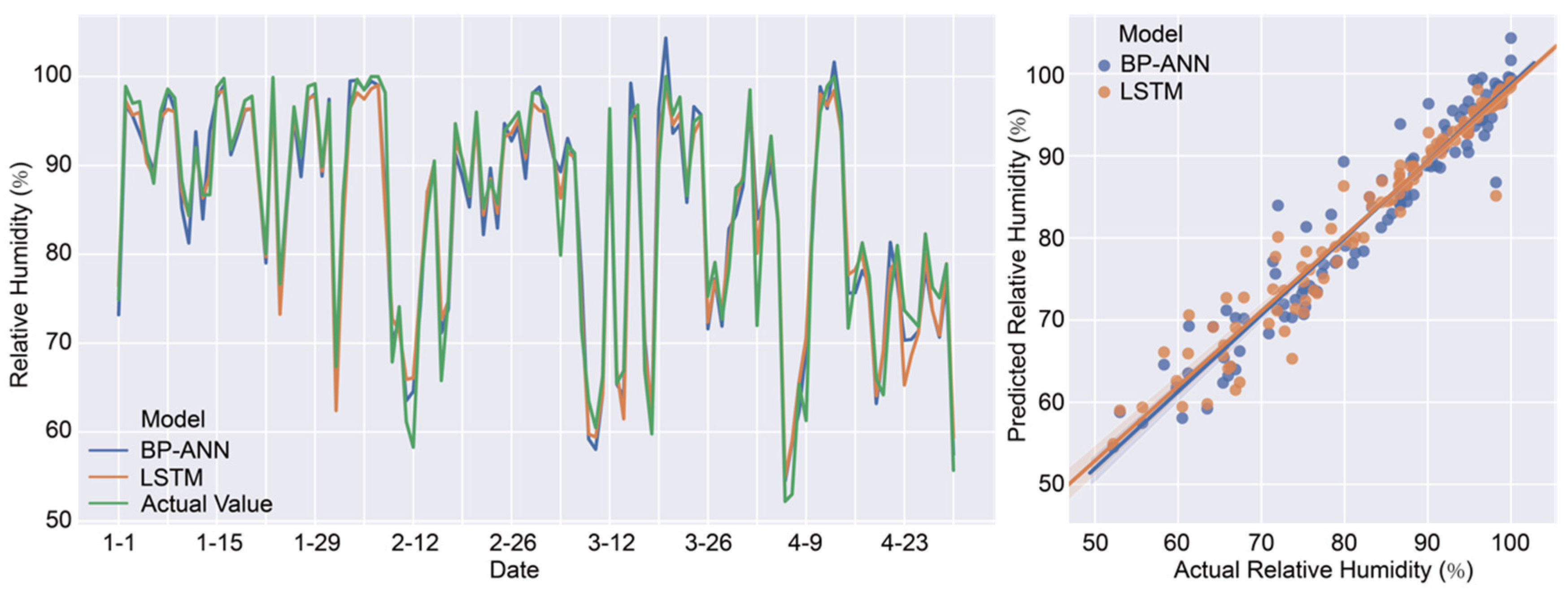
| Real-time prediction | BP-ANN | 96.78% | 99.66% | 3.09% | 2.63% |
| LSTM | 97.48% | 99.66% | 2.59% | 1.92% | |
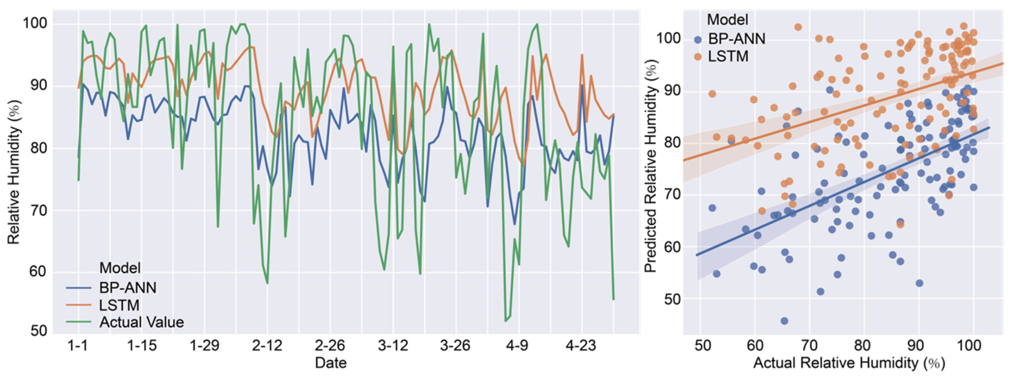
| Characteristic prediction | BP-ANN | 59.00% | 55.65% | 11.40% | 21.54% |
| LSTM | 43.57% | 68.23% | 12.79% | 17.28% | |
Publisher’s Note: MDPI stays neutral with regard to jurisdictional claims in published maps and institutional affiliations. |
© 2022 by the authors. Licensee MDPI, Basel, Switzerland. This article is an open access article distributed under the terms and conditions of the Creative Commons Attribution (CC BY) license (https://creativecommons.org/licenses/by/4.0/).
Share and Cite
Wu, X.; Hou, J.; Hui, J.; Tang, Z.; Wang, W. Revealing Microclimate around Buildings with Long-Term Monitoring through the Neural Network Algorithms. Buildings 2022, 12, 395. https://doi.org/10.3390/buildings12040395
Wu X, Hou J, Hui J, Tang Z, Wang W. Revealing Microclimate around Buildings with Long-Term Monitoring through the Neural Network Algorithms. Buildings. 2022; 12(4):395. https://doi.org/10.3390/buildings12040395
Chicago/Turabian StyleWu, Xibin, Jiani Hou, Jun Hui, Zheng Tang, and Wei Wang. 2022. "Revealing Microclimate around Buildings with Long-Term Monitoring through the Neural Network Algorithms" Buildings 12, no. 4: 395. https://doi.org/10.3390/buildings12040395
APA StyleWu, X., Hou, J., Hui, J., Tang, Z., & Wang, W. (2022). Revealing Microclimate around Buildings with Long-Term Monitoring through the Neural Network Algorithms. Buildings, 12(4), 395. https://doi.org/10.3390/buildings12040395