Insights into Metal Sheet Novelty Detection via Simulated Electromagnetic Ultrasonic Surface Wave

Abstract

Metal sheets have good performance and have been widely used. Different kinds of defects can be generated during the preparation and service of metal plates, which will cause the structural performance of the metal plates to decline, thus requiring structural health monitoring (SHM). This study proposes an electromagnetic ultrasonic (EMUS) surface wave detection technique for metal sheet defects via simulation. The numerical results show that after the excitation parameters of the EMUS transducer are optimized through orthogonal experimental design, the amplitude of the EMUS signal generated is increased by about 80%. The power spectrum density (PSD) of the EMUS response signal is used to detect defects. Compared with the peak-to-peak detection, the accuracy is higher, and the reliability is better. The accuracy of the proposed “central zero-point” method for measuring the time delay of the EMUS signal wave packet is higher than that of the “peak-to-peak amplitude” method and the “vibration starting point” method and is close to the accuracy of the “cross-correlation” method.

1. Introduction

Plate-like metals and their alloys have been widely applied, such as in aircraft fuselages, wings and cabin doors, ships and submarine shells, rails, and storage tanks, etc., due to their good physical and chemical properties and structural strength [1]. In the process of mechanical manufacturing, the forged and shaped metal plates will inevitably have various defects such as cracks, inclusions, and delaminations [2,3,4]. These metal plates will also endure long-term cyclic loading, temperature alternation, and mechanical vibration, leading to the formation of new defects and the further extension of the existing defects, which will then induce structural deterioration. Structural deterioration might cause huge economic loss and affect operating safety. To ensure the safety and reliability of equipment in long-term operation, structural health monitoring (SHM), fault damage early warning, and timely maintenance systems can help to eliminate safety hazards, avoid catastrophic accidents, and reduce maintenance costs [5].

Various non-destructive testing (NDT) techniques have been applied to sheet metal defects, including eddy current testing, X-ray testing, ultrasonic testing, magnetic particle testing, infrared testing, and so on [6,7,8]. The ultrasonic testing method can detect surface and internal defects and accurately determine the position and size of the defects, with simple operation, low cost, and high efficiency. At present, the main excitation method of ultrasound is piezoelectric ultrasound. In recent years, there have been some new excitation methods, such as electromagnetic ultrasound (EMUS), laser ultrasound, air-coupled ultrasound, and so on. Traditional piezoelectric ultrasonic technology needs to use a couplant, which is mainly used in the laboratory testing and is incapable of online testing [9]. EMUS testing is a type of ultrasonic NDT technique that has developed since the 1960s. Unlike the generation mechanism of piezoelectric ultrasound, the excitation and reception process of EMUS is realized through the mutual transformation of electromagnetic force and mechanical force. Therefore, it does not need a couplant. The main detection device of EMUS is the electromagnetic acoustic transducer (EMAT). In addition to avoiding the use of a couplant, EMAT can also conveniently control the excitation parameters of the EMUS transducer to generate multiple modes of ultrasound and change its amplitude, frequency, and propagation direction. What is more, compared with the traditional piezoelectric transducer, the excitation method is more operable and flexible [10].

For EMUS detection of structural defects, researchers have achieved a lot of scientific research results. EMUS technology has been used for pipeline defect detection since its inception. Thompson used Lamb waves excited by EMAT to detect gas pipelines, and the sensitivity of the detection to various design parameters is discussed as well as the amplitude of signals reflected from defects [11]. Cawley considered that when ultrasound propagates along the axial direction of the pipeline, the guided wave can be regarded as a cylindrical Lamb wave. What is more, if the ultrasound propagates along the circumference of the pipeline and when the excitation and reception probes are relatively close, the pipeline under such conditions can be regarded as a flat sheet [12]. Hirao et al. proposed using EMAT to generate shear-horizontal(SH) waves along the circumference of the pipeline to detect corrosion defects in the inner pipeline wall [13]. The SH0 and SH1 waves generated by EMAT can be used to detect defects such as cracks, corrosion, and coating detachment. Gauthier et al. used EMAT to generate multiple modes of SH waves to detect groove defects on the outer surface of the pipeline and performed B-scan imaging of the results [14]. Luo studied the pipeline axial crack detection and its description technology [15]. Zhao studied the quantification of defect features and the mode selection of guided waves by establishing a three-dimensional boundary element model of EMUS. They used the boundary element method (BEM) to calculate the reflection and refraction coefficients of SH waves propagating through the crack. Then, they analyzed the characteristics of the received signal and used SH waves propagating along the pipeline wall to analyze and describe the pipeline pit defect [16,17,18]. Wang found that the vibration amplitude of Rayleigh waves due to the dynamic magnetic field is almost proportional to the reciprocal of the ratio of wire width to spacing interval between neighboring wires (RWWSI), whereas that due to the static magnetic field decreases slowly with the increase of the RWWSI [19]. Li established a three-dimensional model for Rayleigh wave electromagnetic acoustic transducers. Rayleigh waves generated by Lorentz forces due to the static magnetic field and the dynamic magnetic field were calculated [20]. Thring used finite element analysis (FEA) to model the effects of the spatial width of the racetrack generation coil and focused geometry, and no significant difference was found between the focused and the unfocused EMAT response [21]. Jozef developed a pulse excitation and reception system for EMAT, which can drive up to four EMAT coils with a programmable phase delay, to realize the diagnosis and detection of steel plates at high temperatures [22]. Lsla analyzed the possibility of surface defects detection using EMUS phased array technology by combining theoretical derivation and model simulation [23]. Jaime excited orthogonally polarized shear waves by designing an orthogonal coil. They studied different types of crack defects by finite element (FE) analysis and verified the feasibility of orthogonally polarized shear waves for thickness measurement and crack detection [24]. Trushkevych used a small EMAT inspection system to detect surface corrosion defects, and the detection results showed that defects with a length of 1–11 mm and a depth of 0.5–2 mm could be measured [25].

EMUS NDT has achieved a lot of results in excitation coil design, mode analysis, and relevant simulation and experimental research. It can be seen from the above research that one of the main factors restricting the accuracy of EMUS NDT is the corresponding relation between EMUS signals and defect features; on the other hand, the time difference measurement between EMUS wave packets is also an urgent need to solve in defect positioning.

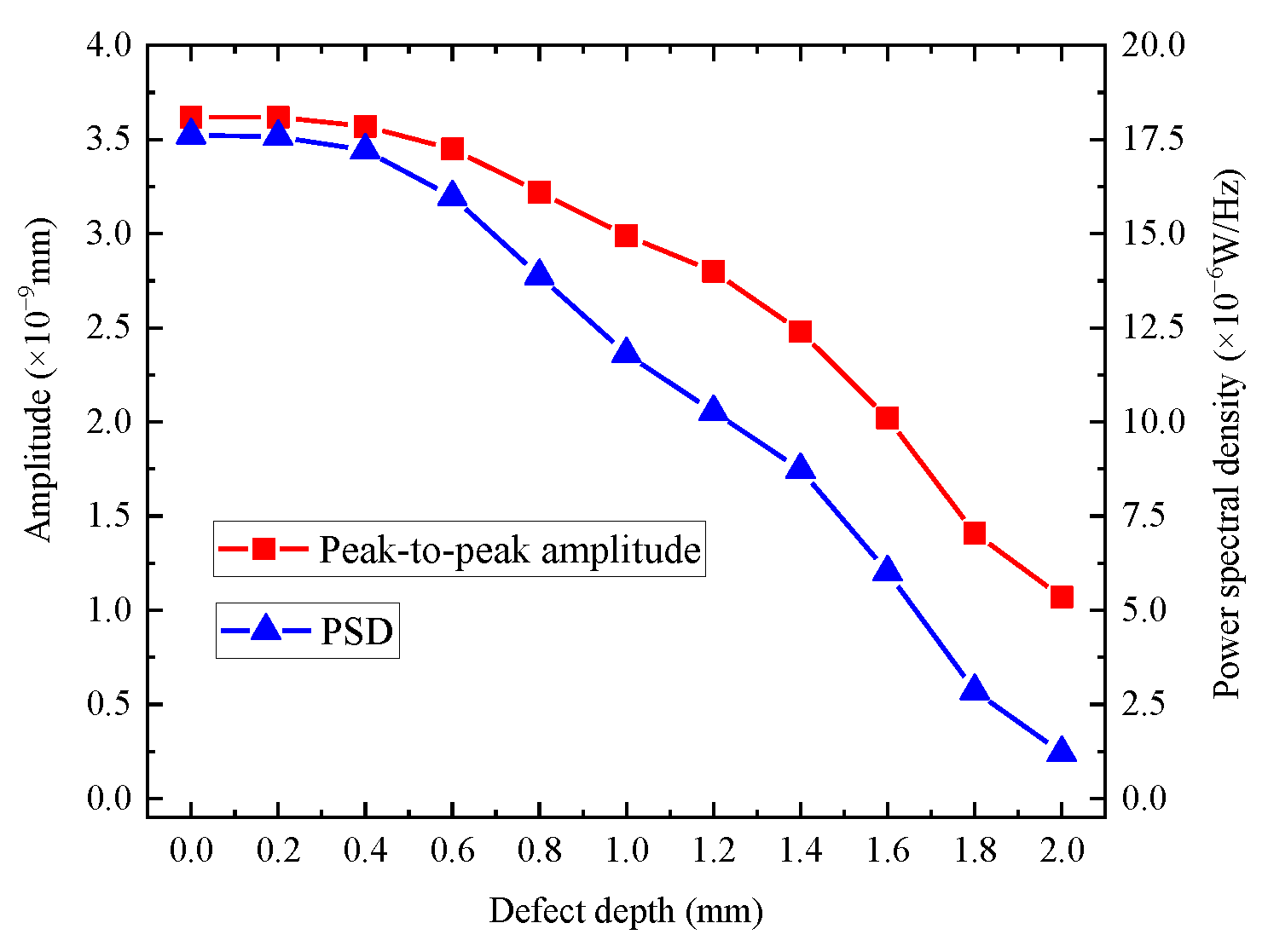
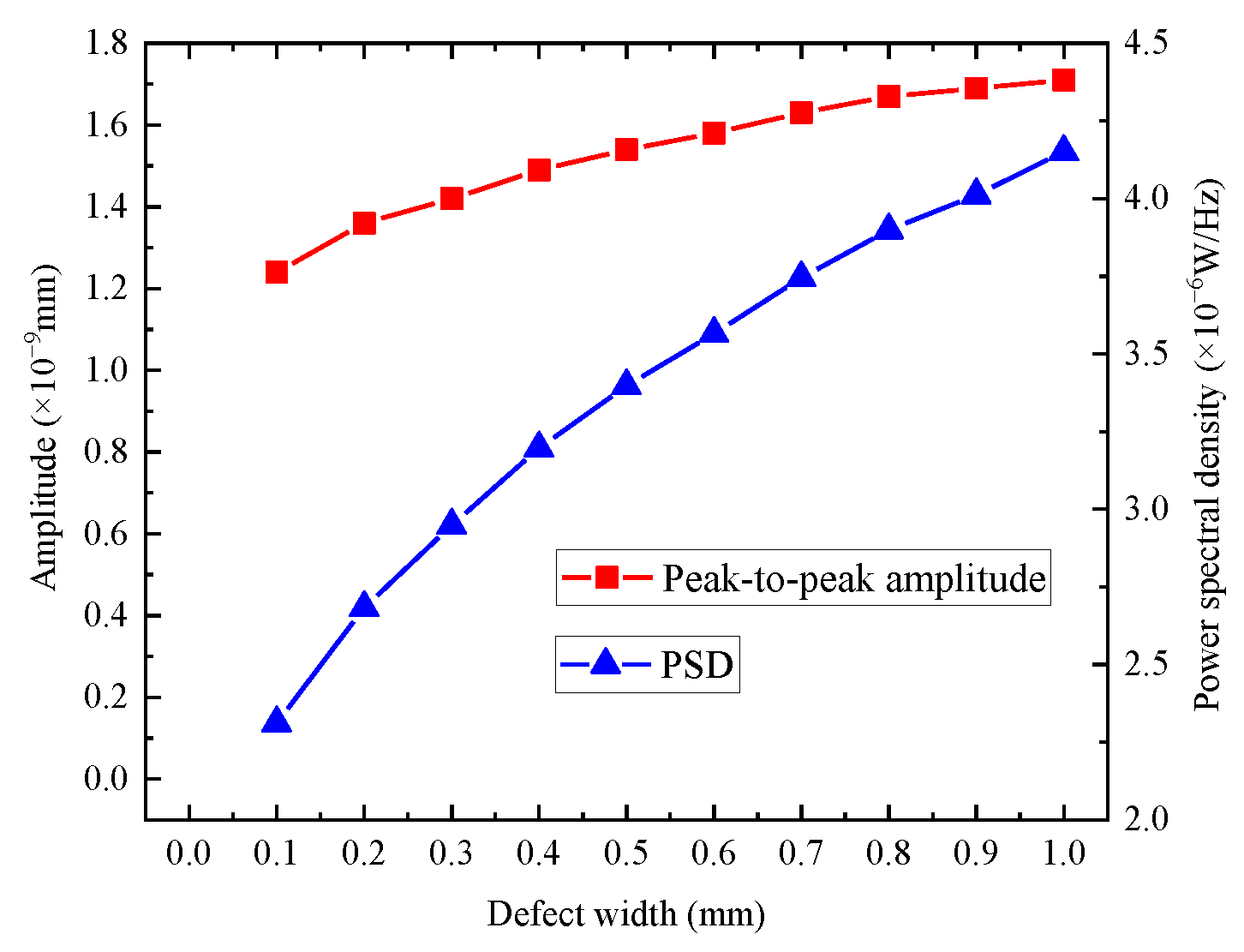
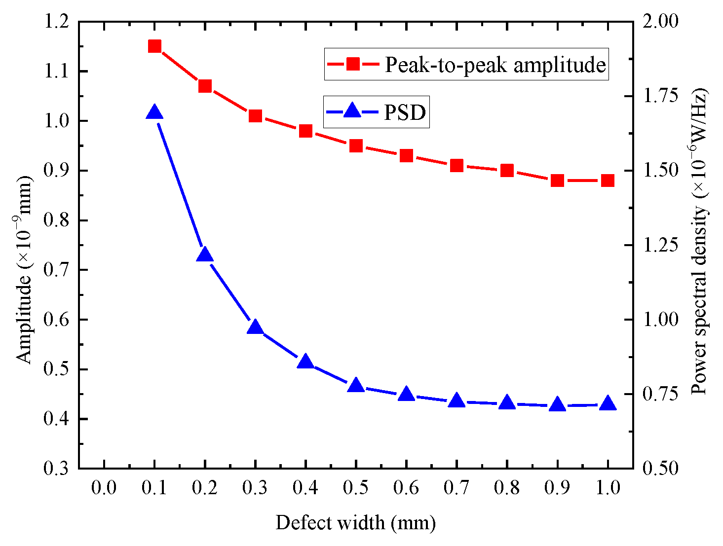
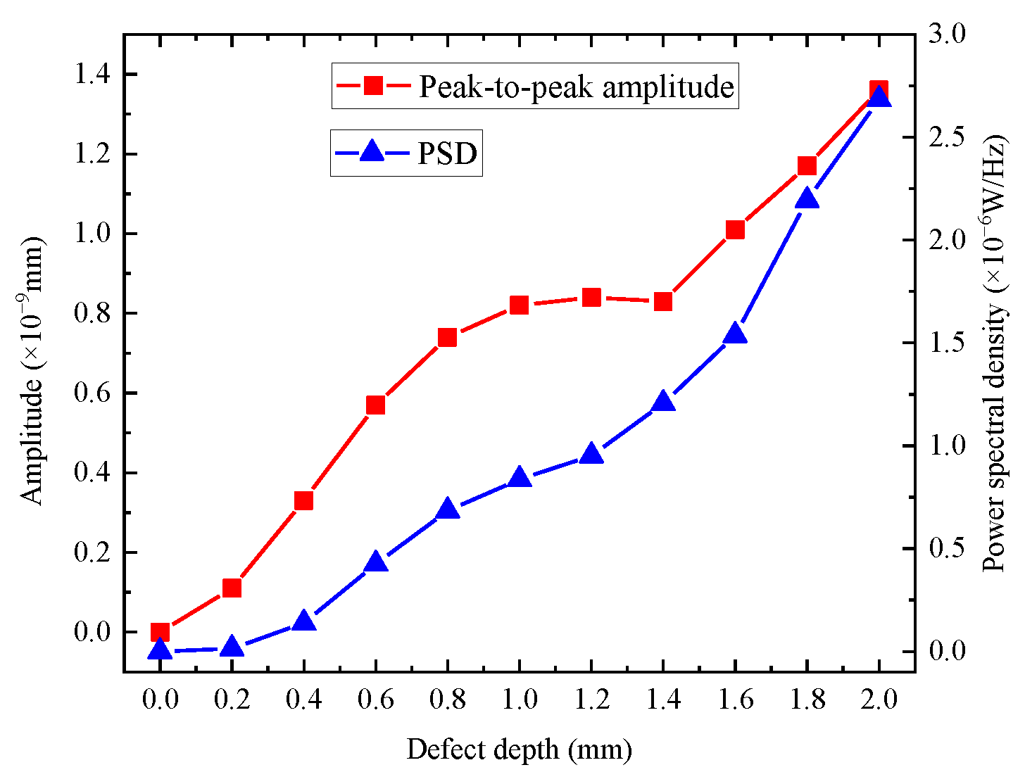
This study simulates the EMUS surface wave detection of metal sheet defects in an aluminum plate. The EMUS energy transduction mechanism of non-ferromagnetic materials based on Lorentz force and the design principle of EMUS surface wave zigzag coils are theoretically analyzed; the electromagnetic field distribution of the EMUS transducer, the propagation depth of surface waves, and the influence of grid accuracy on the EMUS excitation signal amplitude are analyzed based on orthogonal experimental design (OED), and the excitation parameters of the EMUS surface wave transducer are optimized; the comparison of peak-to-peak amplitude and power spectral density (PSD) of the EMUS signal in defect detection is analyzed; a “center zero point” method for measuring the time difference of EMUS wave packet is proposed, and comparisons with the “peak-to-peak” method, the “vibration starting point” method, and the “cross-correlation” method are conducted.

2. Theoretical Background

2.1. Theory of EMUS Transducer

The EMUS transducer based on the Lorentz force is composed of a coil, a magnet, and a non-ferromagnetic test piece. The magnet generally used is a permanent magnet to provide a bias magnetic field, and a high frequency excitation current is applied into the coil to generate an alternating eddy current field. The principle of EMAT exciting EMUS Lamb guided waves in non-ferromagnetic materials is shown in Figure 1, where J_c represents the excitation current, J_e indicates the induced eddy current, B₀ means the horizontal bias magnetic field, F_L indicates the Lorentz force, and h denotes the thickness of the non-ferromagnetic material metal plate.

For the EMUS transducer, the induced alternating eddy current in the skin layer of the test piece will produce alternating Lorentz forces under the action of the bias magnetic field. The Lorentz force acts on the material crystal lattice, causing the mass point in the material to vibrate at the same frequency with the excitation current, thereby generating ultrasonic waves inside the test piece. The above process can be described by the following equations:

$$\frac{1}{\mu }{\nabla }^{2}A-\sigma \frac{\partial A}{\partial t}=-J_{\mathrm{c}}$$

(1)

where A means the vector magnetic potential, σ denotes the conductivity of the material, and J_c represents the source current density, t means the time, µ denotes the magnetic permeability.

$$J_c=\frac{i}{S}+\frac{\sigma }{S}{\displaystyle \underset{S}{\iint }\frac{\partial A}{\partial t}}ds$$

(2)

where i means the total current; and S denotes the cross-sectional area of the coil.

Substituting Equation (2) into Equation (1) shall obtain

$$\frac{1}{\mu }{\nabla }^{2}A-\sigma \frac{\partial A}{\partial t}+\frac{\sigma }{S}{\displaystyle \underset{{\Omega }_c}{\iint }\frac{\partial A}{\partial t}}ds=-\frac{i}{S}$$

(3)

$$Je=-\sigma \frac{\partial A}{\partial t}$$

(4)

$$f_L=B_0\times Je$$

(5)

where f_L represents the Lorentz force, and B₀ means the bias magnetic field.

2.2. Design Principle of Surface Wave Zigzag Coil

The zigzag coil is designed based on the wave coherence principle. When the coil turn distance is half of the ultrasonic wavelength λ, the ultrasonic waves excited by each single coil turn satisfy the wave coherence principle, and its excitation and reception efficiency is the highest. In this situation, the wavelength and the coil turn distance meet the following condition [26]:

$$D=(2n+1)\lambda , n=0, 1, 2\dots$$

(6)

where D means the coil turn distance of the zigzag coil, and λ represents the wavelength of the guided wave. In general, n = 0, and D = λ.

3. Model Description

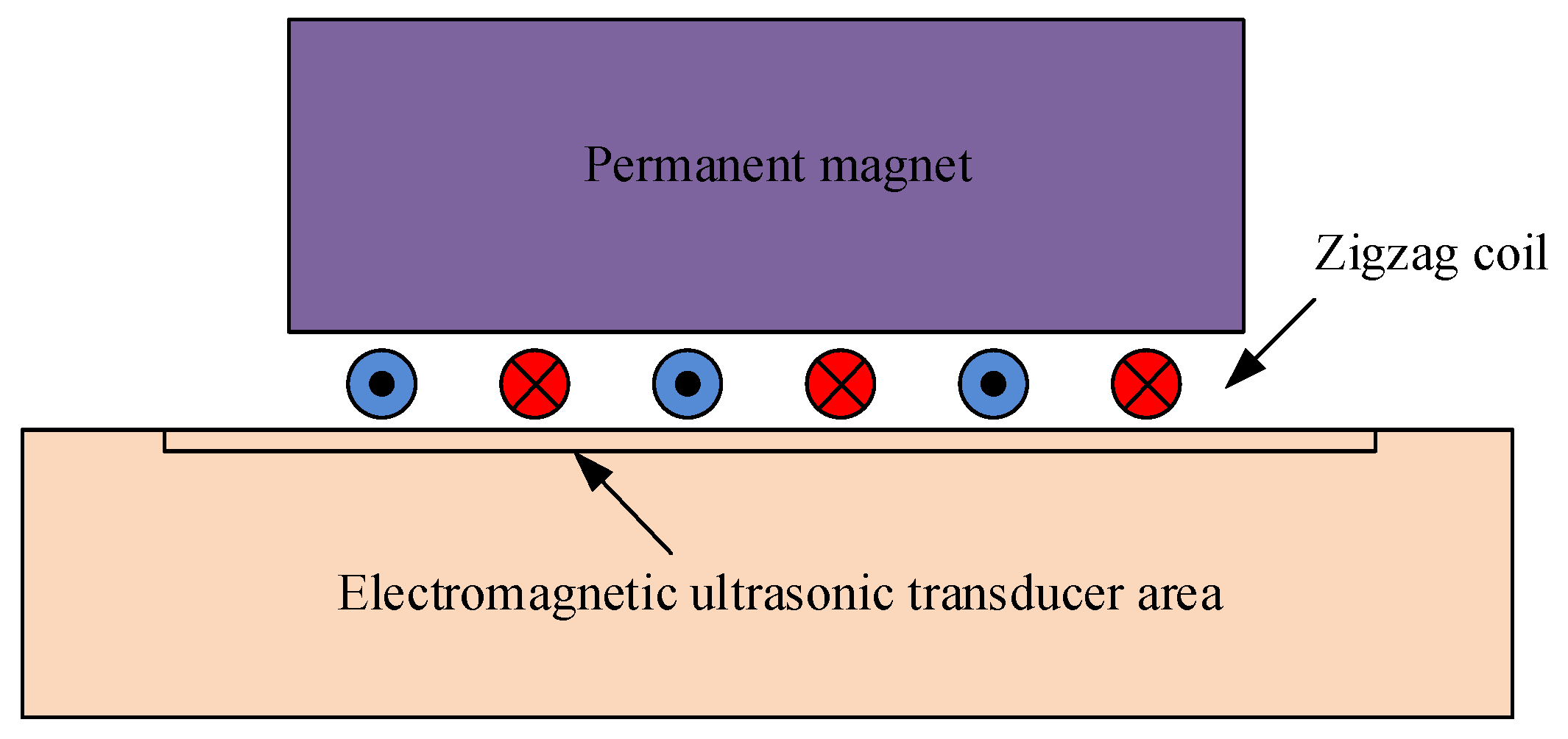
Based on COMSOL Multiphysics software 5.4, a two-dimensional model for EMUS surface wave detection of metal sheet defects was established, as shown in Figure 2. The model mainly includes a thin metal plate (aluminum plate), an EMAT module, and an air field. The size of the aluminum plate is 500 mm × 10 mm. The air field above the model is also 500 mm × 10 mm. 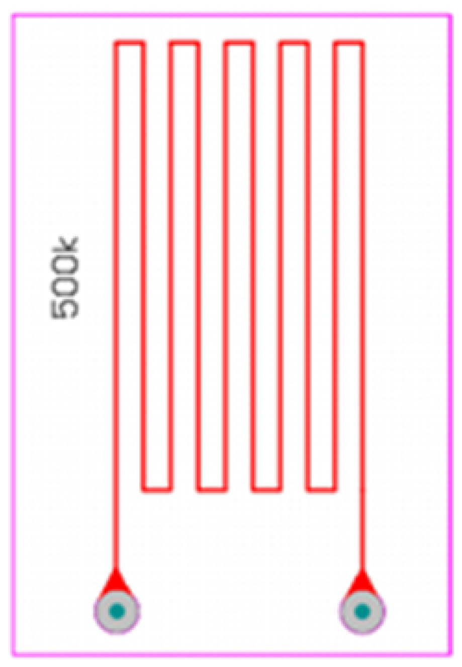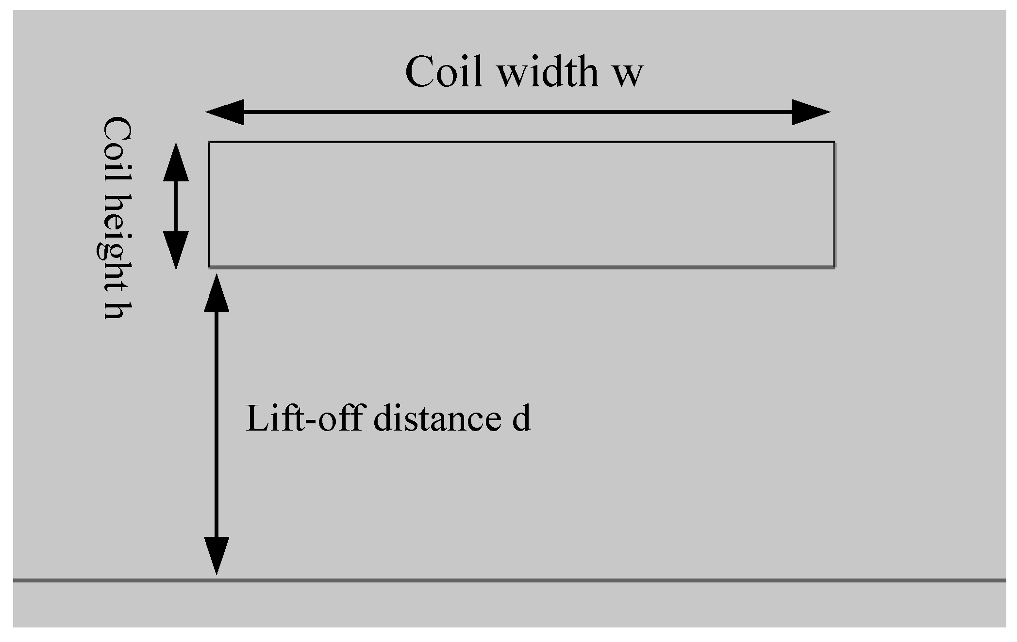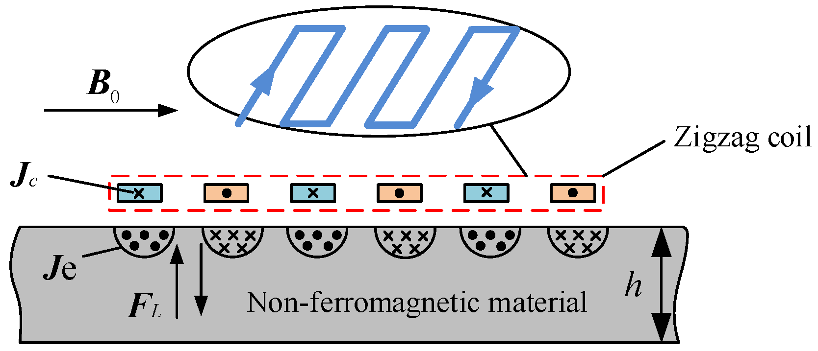The enlarged view of the EMAT module is shown in Figure 3. The EMAT module is composed of a permanent magnet and a zigzag excitation coil. The permanent magnet is made of NdFeB with a size of 30 mm × 7 mm. The excitation coil is a 3-turn zigzag coil with a turn width of 1.0 mm and a turn thickness of 0.2 mm, the lift-off distance is 0.5 mm, and the coil turn distance is 2.98 mm. A schematic of the coil geometry is shown in Figure 4. Surface waves generally refer to signals propagating through the surface of a semi-unbounded area. To reduce the influence of the reflected echoes of the left, right, and bottom end faces on the received signals, the left, right, and bottom end faces are set as low reflection boundary.

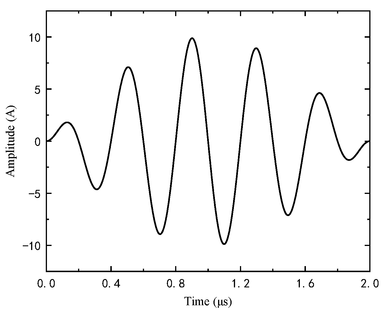
In the simulation, the calculation step is set to T/20; T is the time period of the excitation signal; the calculation time is 200 T; the “generalized alpha” method is selected in the solution process. The excitation current in the coil is a sinusoidally modulated tone-burst signal, as shown in Figure 5. Each cycle contains five fundamental frequency signals; I_max is the amplitude of the excitation signal; I_max = 10 A; the current signal equation is as follows:

$$I=\sin (2\times \pi \times f\times t)\times \sin (2\times \pi \times f\times t/10)\times (t<5\times \mathrm{T})\times I_{\max }\left[A\right]$$

(7)

The density of the FE mesh directly determines the calculation accuracy of the FE model. The finer the mesh size is, the more accurate the calculation result will be. To improve the calculation accuracy, this study refined the skin depth area of the aluminum plate where the electromagnetic field energy is concentrated and changed drastically during the EMAT transduction process. The skin depth δ of the aluminum plate is as follows:

$$\delta =\sqrt{\frac{{\rho }_m}{\pi {\mu }_0{\mu }_{m}f}}$$

(8)

where ρ_m means resistivity of aluminum plate, and ρ_m = 2.62 × 10⁻⁸ Ω/m; μ₀ represents vacuum permeability, and μ₀ = 4π × 10⁻⁷ H/m; μ_m denotes the relative permeability of the aluminum plate, and μ_m = 1; f indicates excitation current frequency, and f = 500 kHz.

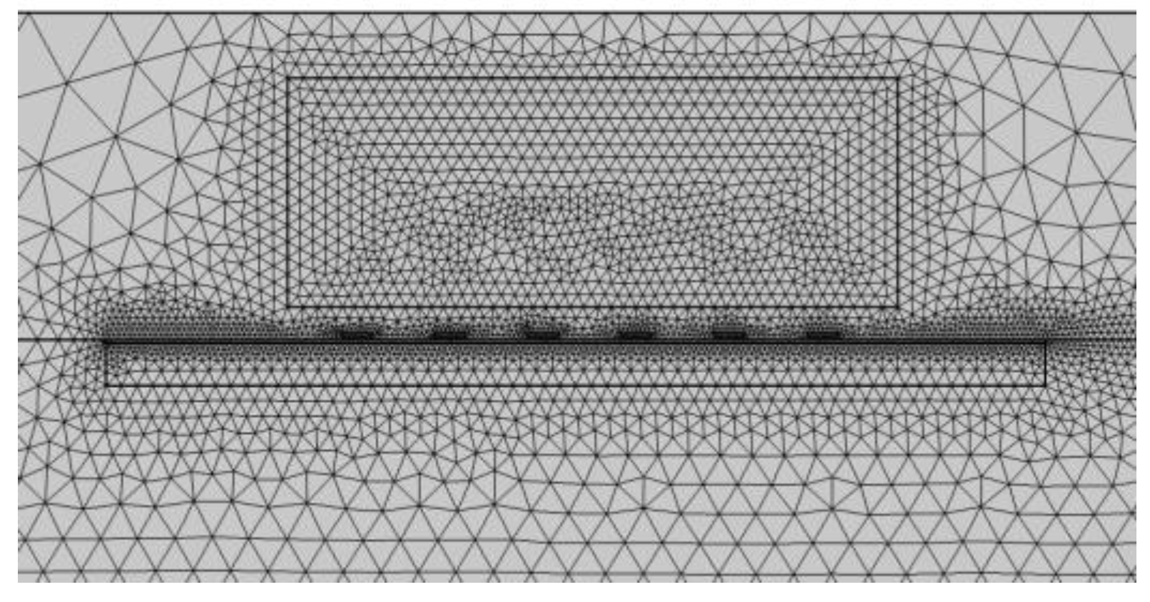
Substituting the above parameters into Equation (8), the skin depth in the aluminum plate is 115.2 μm. In the process of dividing the mesh grid, at least two layers of grids need to be set in the skin depth area. When the mesh size is set according to this principle, the mesh density of the skin depth area is extremely high. If the whole model is meshed according to this principle, the calculation amount will increase exponentially. The calculation accuracy requirement of the air domain is not high; thus, the mesh size of this part can be set larger. Therefore, the calculation complexity of the whole model is mainly determined by the mesh size of the aluminum plate domain. The influence of the mesh size of the aluminum plate domain on the calculation accuracy is mainly reflected in the wave packet shape, wave speed, and amplitude of the surface wave. From the comparison of the simulation results under different mesh accuracy, it can be obtained that when the grid is large, the wave packet composition of the surface wave is more complex, the wave velocity is smaller (compared with the actual wave velocity), and the wave amplitude is also smaller, as shown in Figure 6 and Figure 7. Comparing the results of different mesh size, the maximum size of the aluminum plate domain is set to 1.5 mm. When the mesh size is smaller than 1.5 mm, further refinement hardly affects the calculation result. Considering that the wavelength of the surface wave in this model is about 3 mm, it can be concluded that when the mesh size is less than half the wavelength of the surface wave, the calculation result is accurate. To reserve a certain margin, the maximum mesh size of the aluminum plate domain is set to 1.2 mm. The element number of the whole model is about 20,000 after the gradual refinement of different domains. If the mesh grid is divided according to the principle of skin layer, the element number of the whole model will reach 284,000. Gradual mesh grid refinement can ensure calculation accuracy, reducing the complexity of the model and the calculation amount. Considering the intensity and transduction severity of the electromagnetic field decrease rapidly as the plate depth increases, the mesh grid at a distance from the probe gradually becomes large. After the mesh grid is refined according to the above principle, the mesh division of the whole model is shown in Figure 8.

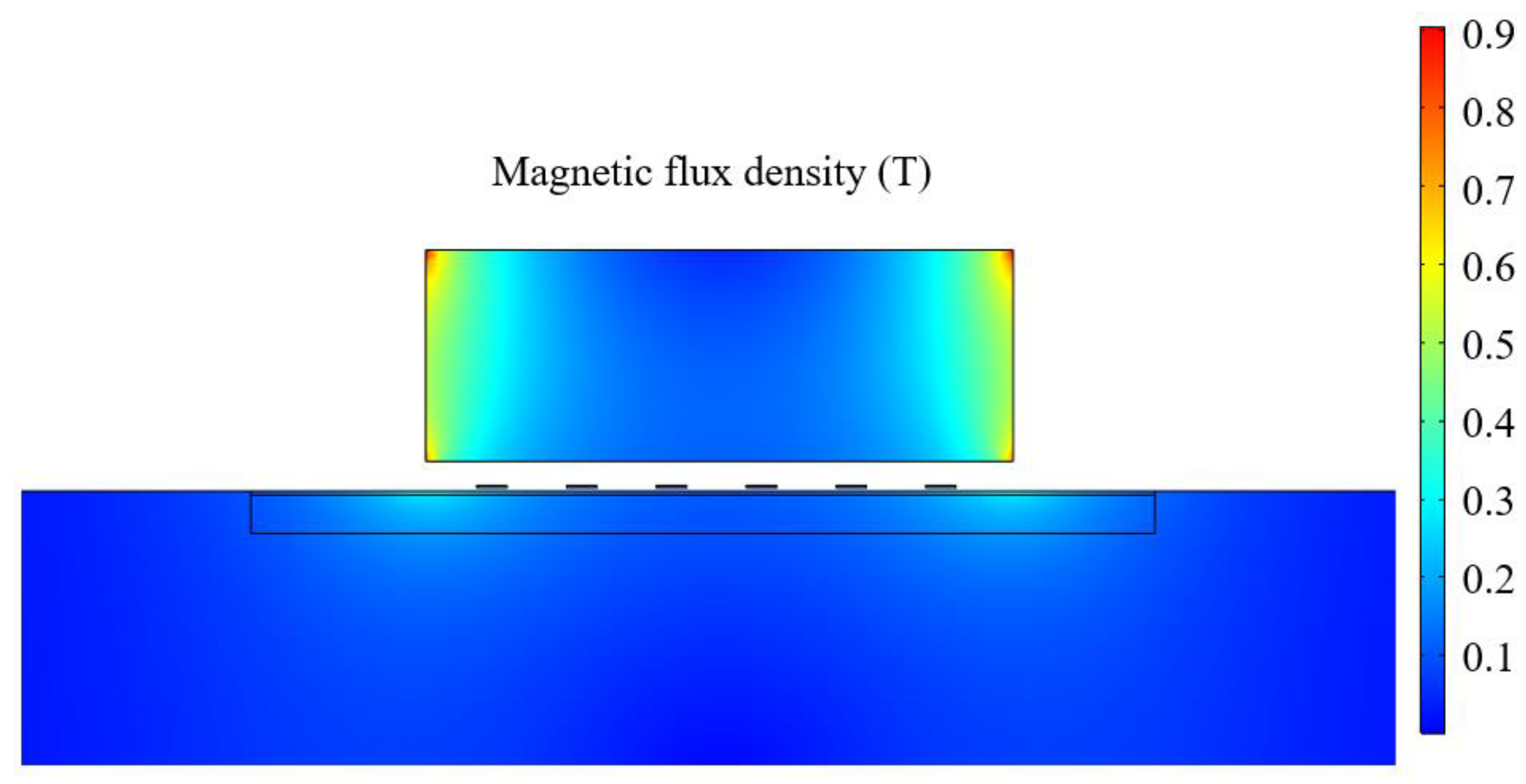
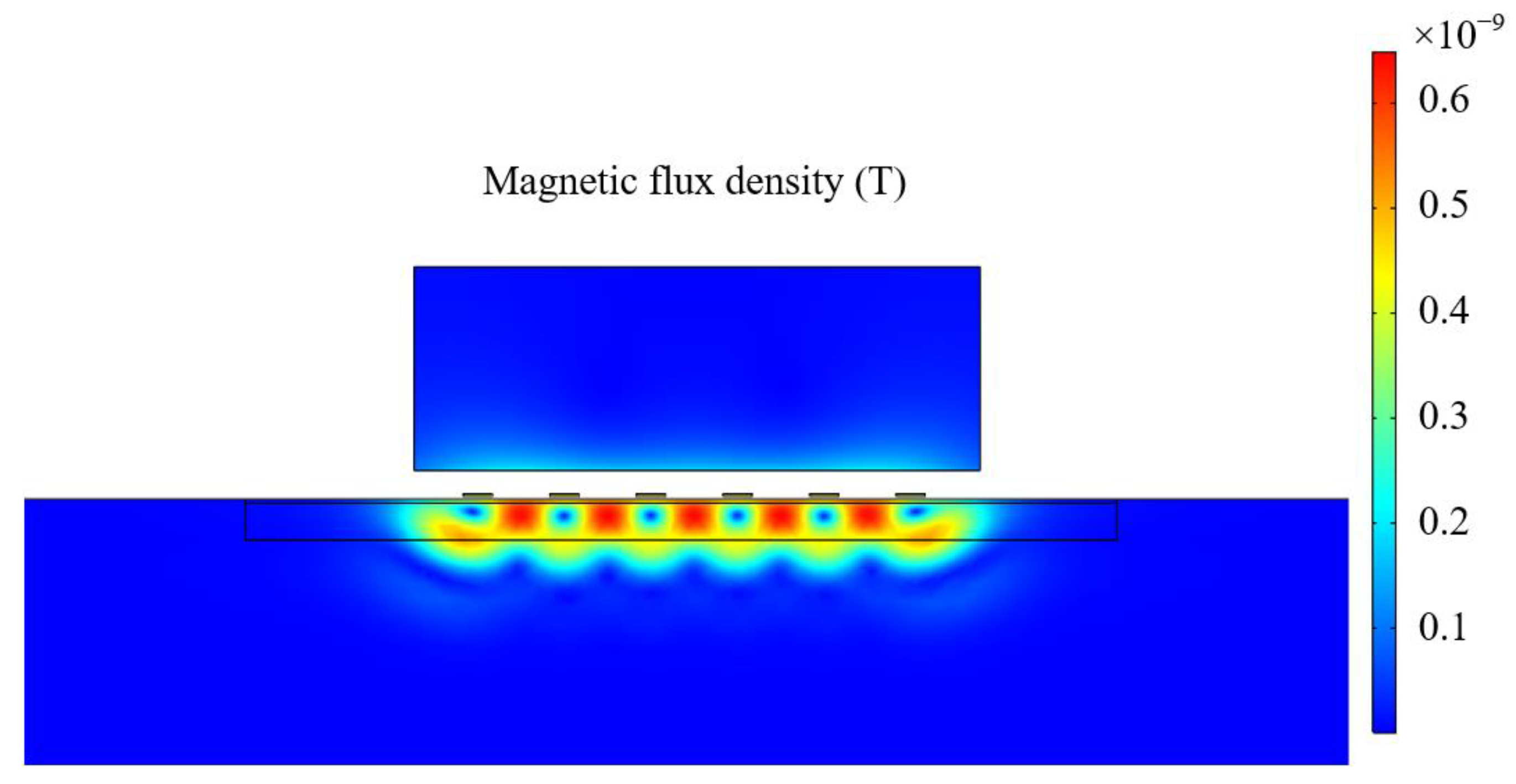
Figure 9 and Figure 10 are the distribution diagrams of the magnetic field generated by the permanent magnet and the excitation coil separately. Comparing Figure 9 and Figure 10, the magnetic field generated by the permanent magnet in the aluminum plate is about (0.1, 0.4) T, while the magnetic field generated by the excitation coil in the aluminum plate is about 4 × 10⁻⁹ T. The intensity of the magnetic field generated by the permanent magnet is much greater than that of the excitation coil. This is why the magnetic field of the excitation coil can be ignored when analyzing the particle vibration in the EMAT transduction process. It can be obtained from the magnetic field distribution of the permanent magnet that the magnetic field intensity in the area where the excitation coil is located is basically the same, which can eliminate the influence of the uneven bias magnetic field on the EMAT transduction process. What is more, it can be obtained from the magnetic field distribution of the excitation coil that the magnetic field below the coil turns is smaller than that of the region between two adjacent coil turns, since the magnetic field generated by the coil is distributed in a circular shape.

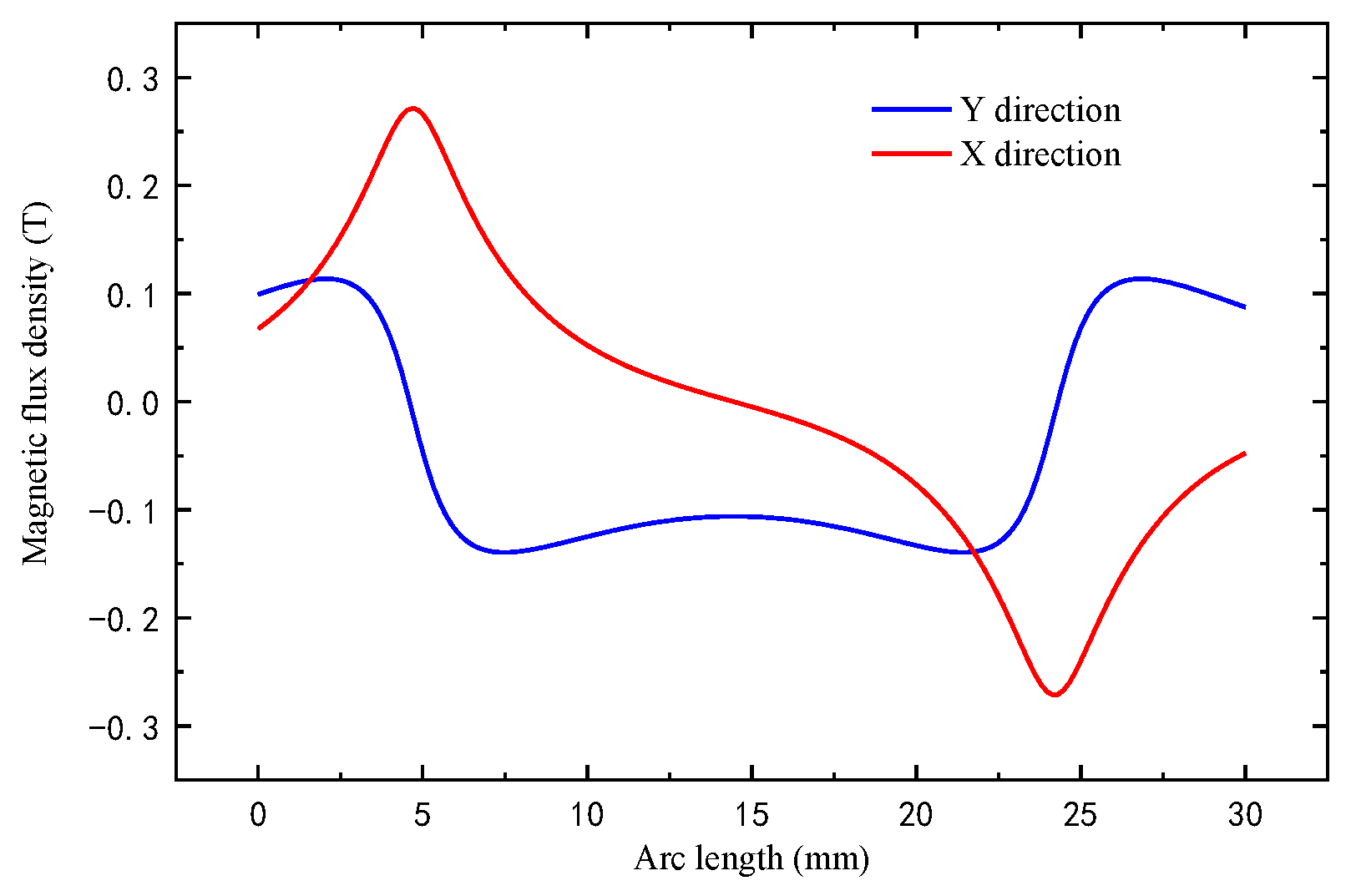
Figure 11 and Figure 12 show the bias magnetic field and eddy current field of the EMAT. The width of the magnet is 20 mm. Figure 11 shows the magnetic flux density in x and y directions of the magnet at 0.01 mm depth in the aluminum plate. It can be obtained from Figure 11 that the middle part of the magnet mainly produces a vertical magnetic field, and the vertical magnetic density at the center position is the weakest and gradually increases to both sides. On both sides of the magnet, due to the edge effect, there are strong horizontal magnetic fields on the left and right sides of the magnet center with opposite directions. The surface wave includes in-plane displacement and out-plane displacement. 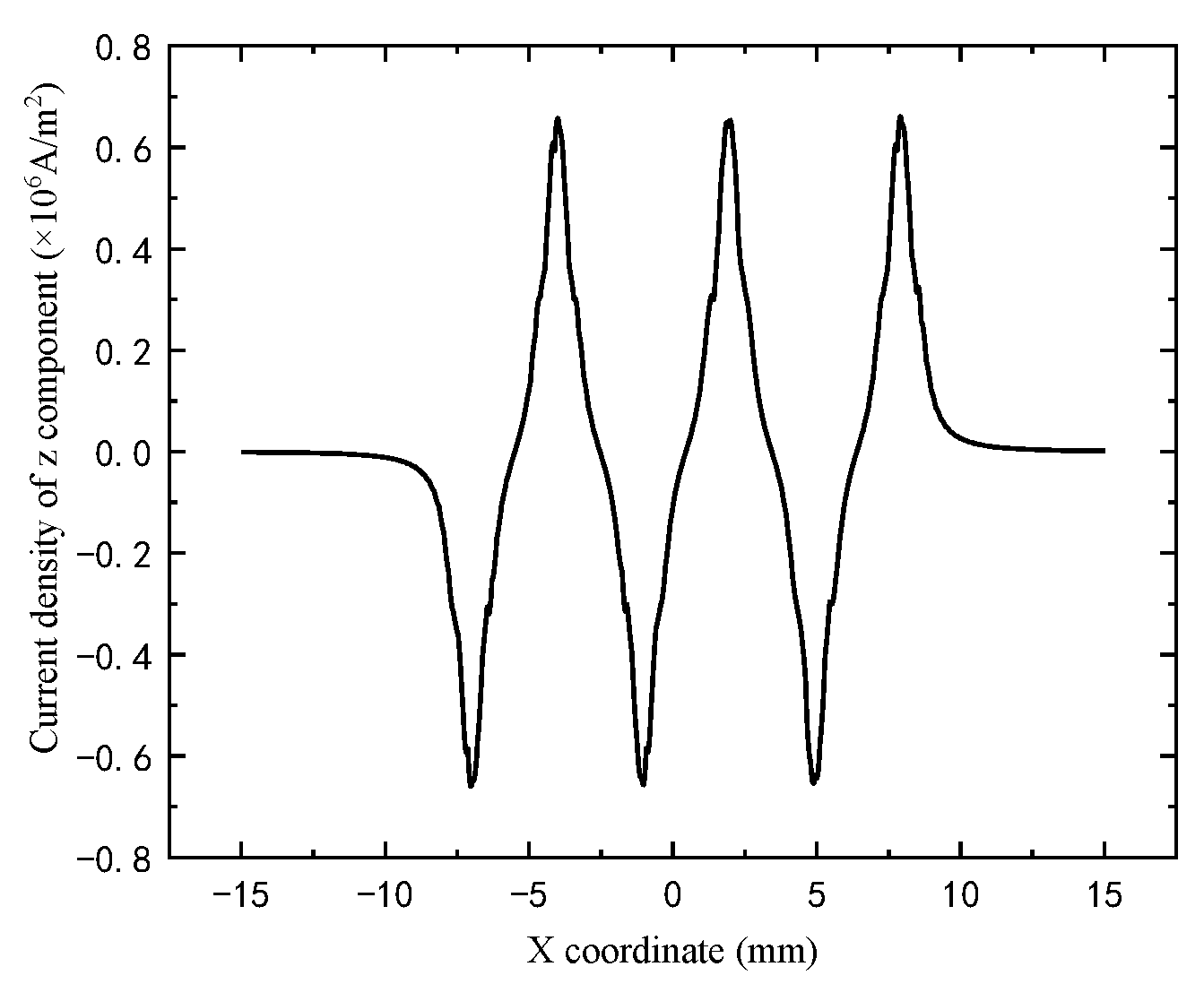The x-direction magnetic field mainly produces out-plane displacement of the surface wave, and the y-direction magnetic field mainly produces the in-plane displacement. The eddy current distribution in the aluminum plate under the excitation coil is shown in Figure 12. Since the current direction of the two adjacent wires of the zigzag coil is opposite, the direction of the eddy current generated in the aluminum plate is also opposite, and the maximum value of the eddy current appears below each coil wire center.

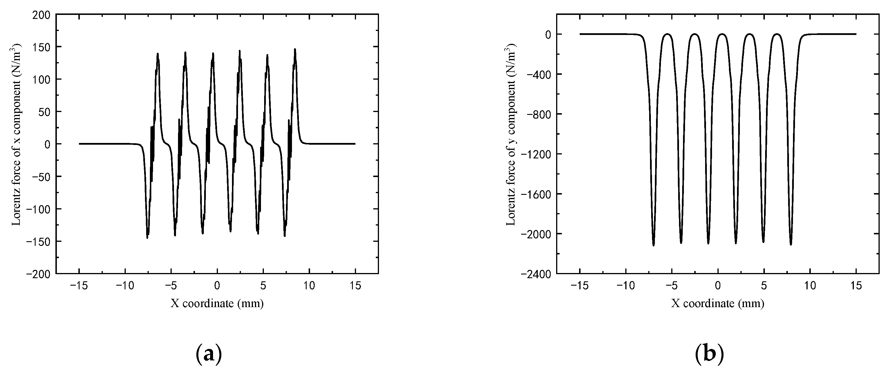
Figure 13 shows the distribution of the Lorentz force in the x-direction and y-direction produced by the interaction of the induced eddy current and the magnetic field in the skin depth of the aluminum plate. The rectangular magnet mainly provides a vertical magnetic field, so the Lorentz force generated in the aluminum plate by the EMAT is mainly in the x direction. Moreover, due to the edge effect of the magnet, a large vertical Lorentz force is generated in the aluminum plate below the edge of the magnet.

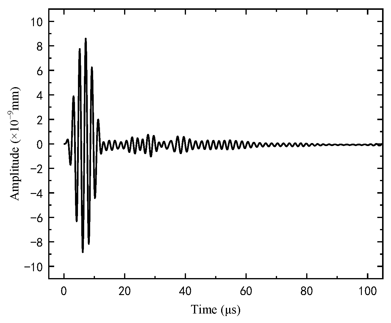
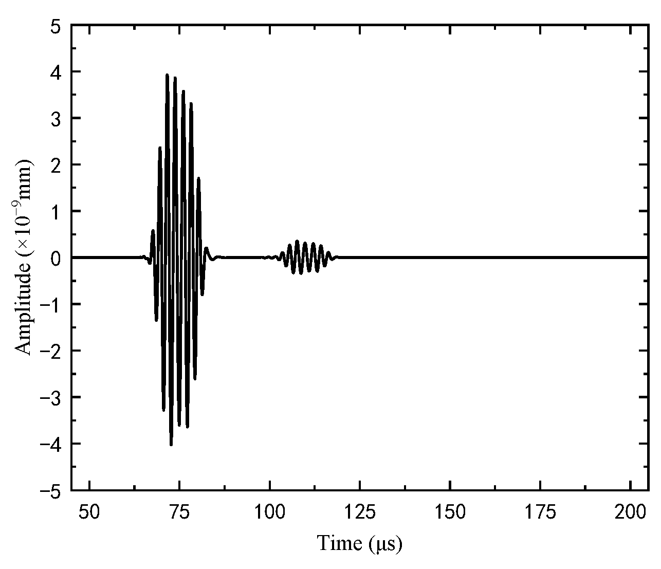
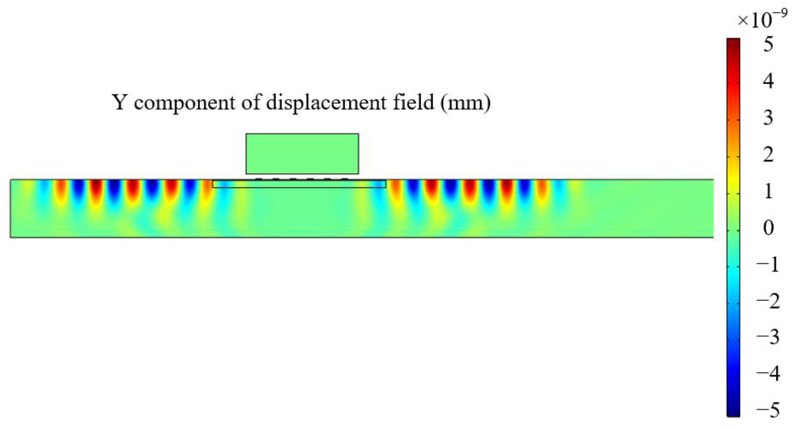
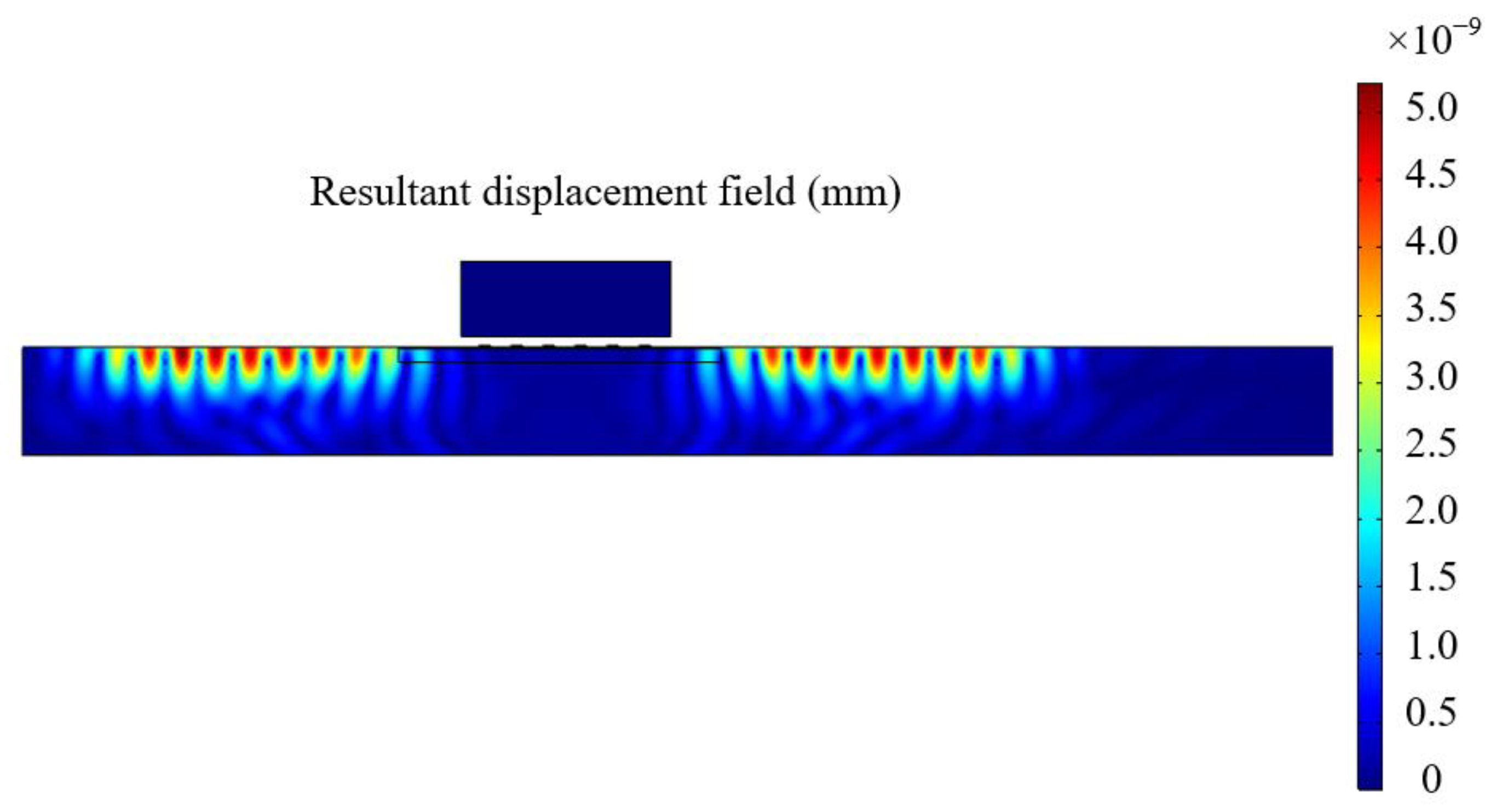
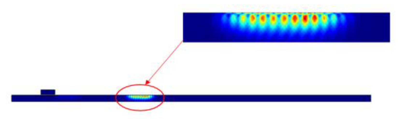
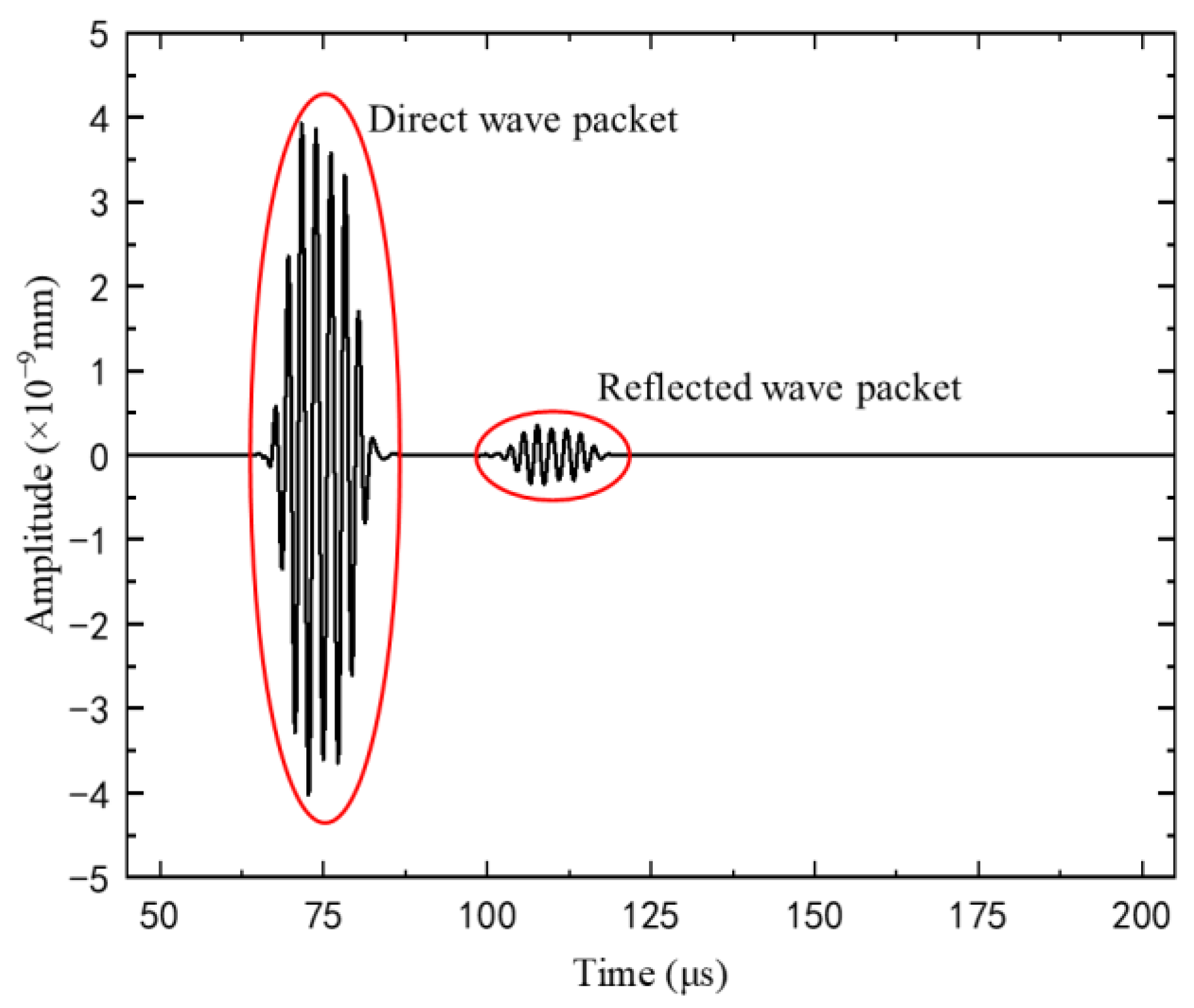
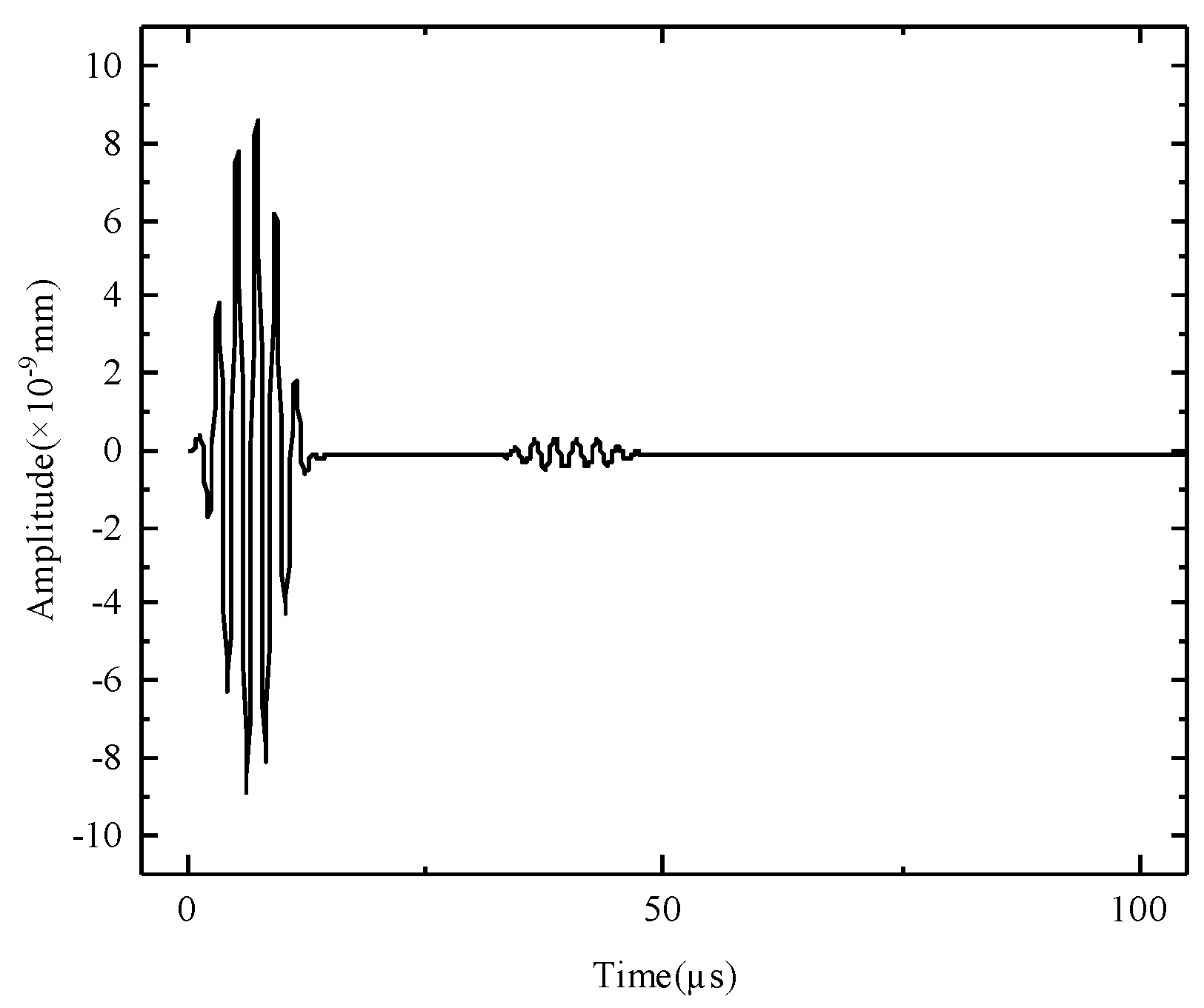
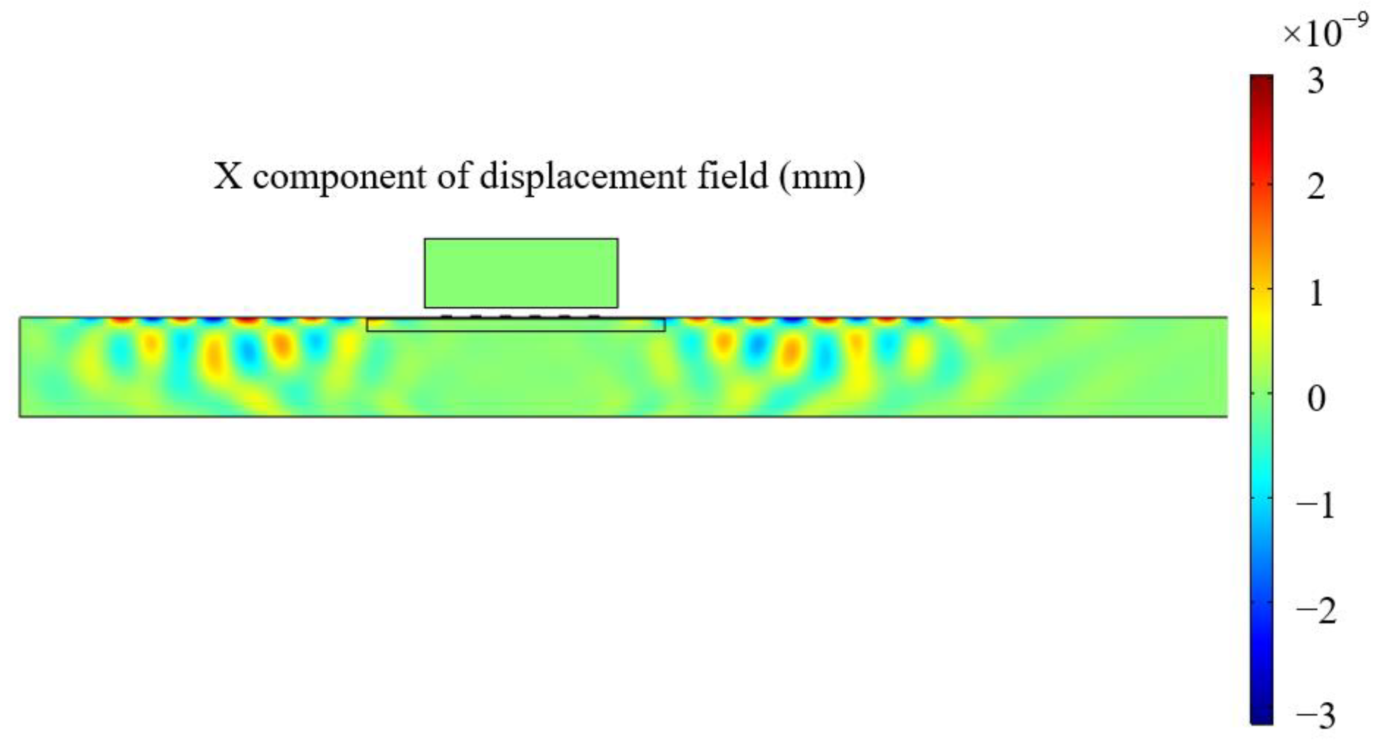
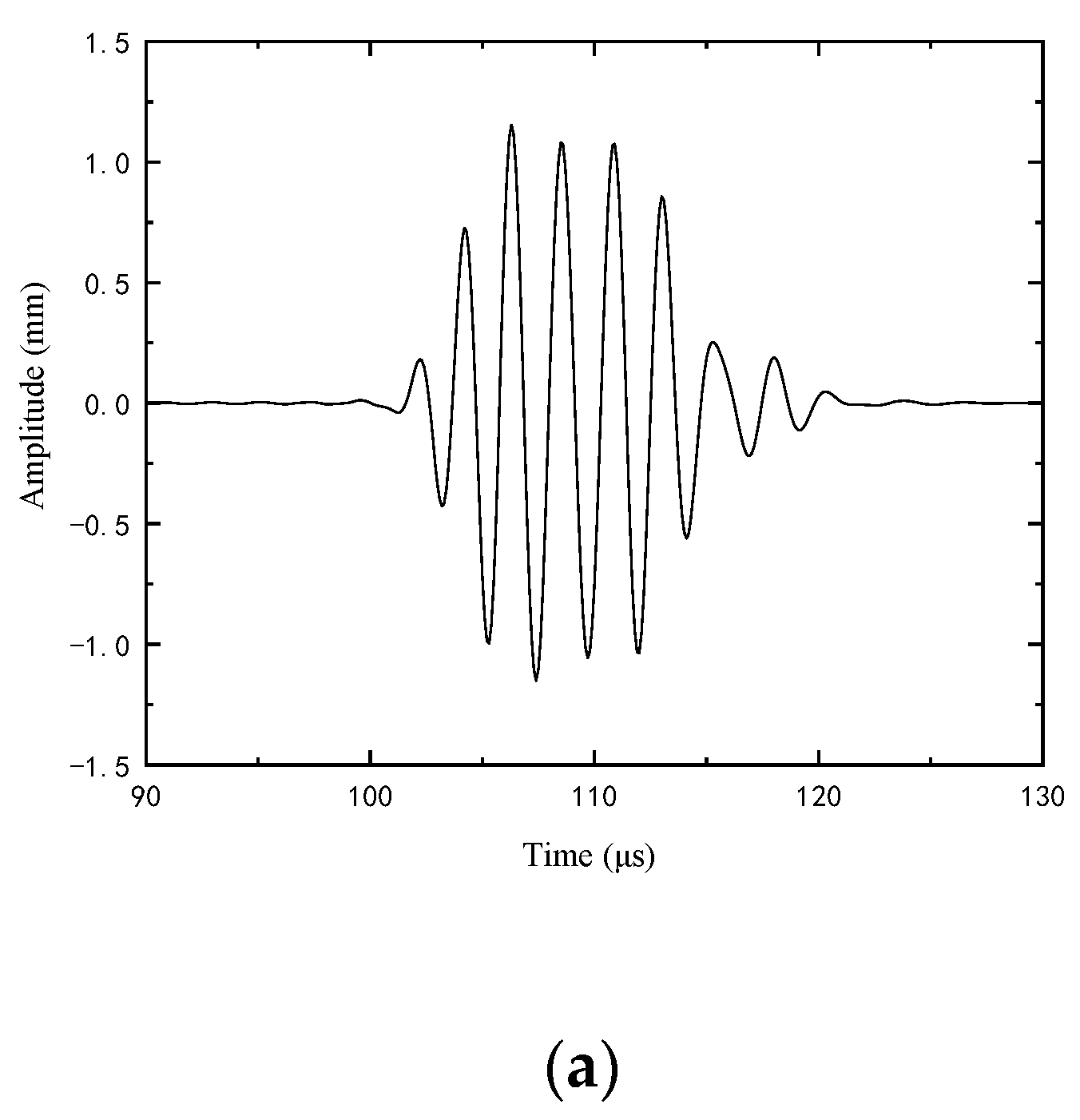
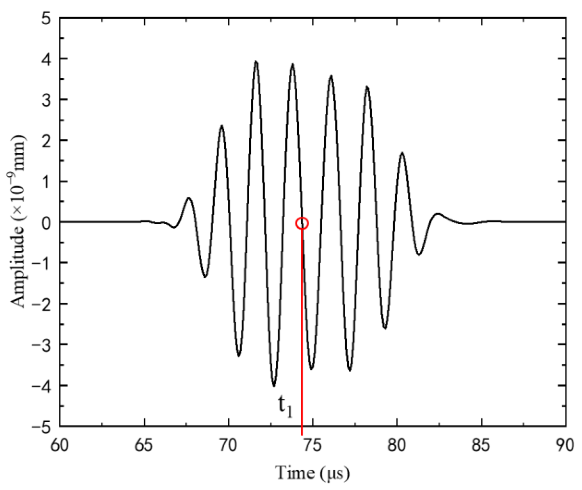
Figure 14 shows the time-domain waveform of the EMUS signal received at point (200, −1). The first wave packet is the direct wave of the excitation signal, and the second wave packet is the reflection wave from the left end surface. It can be calculated from the length of the aluminum plate and the model parameters that the propagation velocity of the surface wave in the aluminum plate is 2890 m/s. The acoustic field of the EMUS signal in the aluminum plate is shown in Figure 15, Figure 16 and Figure 17 at time 1.5 × 10⁻⁵ s. Figure 15 is the out-plane displacement, Figure 16 is the in-plane displacement, and Figure 17 is the resultant displacement. The surface wave excited by this model is mainly out-plane displacement, and the in-plane displacement is small because the permanent magnet mainly provides a vertical magnetic field. Due to the edge effect of the permanent magnet, there is also little horizontal component in the magnetic field, which is the reason for the low-amplitude in-plane displacement in the acoustic field.

4. Results Analysis

4.1. Optimization of EMAT Excitation Parameters

The main factors affecting the amplitude of EMUS surface wave are magnetic field, excitation current, and coil parameters. The magnetic field and excitation current are positively correlated with the amplitude of the surface wave. The magnetic field and excitation current is usually set to the maximum according to the external conditions. Therefore, this section mainly studies the influence of coil parameters on surface wave amplitude. As shown in Figure 18, the coil parameters include coil thickness, width, and lift-off distance. According to the common specifications of EMAT in aluminum plate and current coil manufacturing level, the value range of each factor can be determined in

Table 1. The value range of the three parameters to be optimized.

Lift-Off Distance (mm)	Coil Width (mm)	Coil Thickness (mm)
0.1	0.5	0.1
0.2	1.0	0.2
0.3	1.5	0.3
0.4	2.0	0.4

. The three parameters affect each other. To determine the optimal coil parameter combination, 4³ tests are required, which requires a huge amount of calculation.

To obtain the optimal coil parameter combination and analyze the influence of each parameter individually on surface wave amplitude, this study adopted the orthogonal experiment method to optimize the coil parameters. Orthogonal experimental design is a design method for studying multi-factors and multi-levels. Some representative points are selected from the overall test for experiments based on orthogonality. These representative points have the features of uniform dispersion, regularity, and comparability. Orthogonal experimental design is the main method of fractional factorial design, and it is a highly efficient, fast, and economical experimental design method. For tests with three parameters and each parameter with four levels, 64 experiments are required in the full test. However, if the orthogonal experiment design method is adopted, only 16 experiments are required, which greatly reduces the calculation amount.

The commonly used orthogonal test tables do not have the three-parameter four-level table. By removing the last two columns from L₁₆ (45), the five-parameter four-level orthogonal test table, the three-parameter four-level orthogonal test table can be obtained.

Table 2. Value combinations of three-parameter four-level orthogonal test.

Numerical Order	Parameter 1	Parameter 2	Parameter 3
1	1	1	1
2	1	2	2
3	1	3	3
4	1	4	4
5	2	1	2
6	2	2	1
7	2	3	4
8	2	4	3
9	3	1	3
10	3	2	4
11	3	3	1
12	3	4	2
13	4	1	4
14	4	2	3
15	4	3	2
16	4	4	1

shows the value combinations of the three-parameter four-level orthogonal test. Experiments were carried out according to the value combinations in Table 2, and the corresponding EMUS received signal amplitudes of different value combinations are shown in

Table 3. Received signal amplitude of different value combinations.

Value	Amplitude (×10−9 mm)	Value	Amplitude (×10−9 mm)
111	8.08	313	5.87
122	8.18	324	5.98
133	7.27	331	6.21
144	6.20	342	5.04
212	6.87	414	5.56
221	7.66	423	5.50
234	6.18	432	5.18
243	5.54	441	4.77

.

The commonly used orthogonal test tables do not have the three-parameter four-level table. By removing the last two columns from L₁₆ (45), the five-parameter four-level orthogonal test table, the three-parameter four-level orthogonal test table can be obtained. Table 2 shows the value combinations of the three-parameter four-level orthogonal test. Experiments were carried out according to the value combinations in Table 2, and the corresponding EMUS received signal amplitude of different value combinations are shown in Table 3.

From the comprehensive comparability of the orthogonal experiment, the influence of each parameter on signal amplitude could be obtained by calculating the arithmetic mean value of the signal amplitude ki of each parameter at the same level (where i represents the serial number of the value level of each parameter, i = 1, 2, 3, 4). By analyzing the influence of lift-off distance, coil width, and thickness on the amplitude of the received signal (Figure 19, Figure 20 and Figure 21), the following conclusions could be obtained: the amplitude of received signal gradually decreased with the increase of lift-off distance and coil thickness; it first increased and then decreased with the increase of coil width, and when the received signal amplitude was maximal, the coil width was about 1/3 of the coil turn distance. The best value combination of excitation parameters was 121, that is, a lift-off distance of 0.1 mm, a coil width of 1 mm, and a coil thickness of 0.1 mm. The time domain comparison of the received signal of the optimized parameters and the excitation parameters commonly used in previous simulations is shown in Figure 22. As shown in Figure 22, after the orthogonal test optimization, the received signal amplitude is significantly enhanced by about 80%.

4.2. Surface Wave Attenuation with Propagation Distance and Depth

Figure 23 shows the amplitude of the EMUS surface wave received at 1 mm depth positions in the aluminum plate. The attenuation of the surface wave was very small when it propagated in the aluminum plate. After the ultrasonic signal propagated a 350 mm distance, the attenuation of the amplitude was only 1.16 × 10⁻⁹ mm, and the loss was about 25.7%. It can be estimated that the complete attenuation distance of surface wave in the aluminum plate was about 1400 mm. When the ultrasonic signal propagated a 1000 mm distance, the signal attenuation was 70% of the excitation signal. Effective detection could still be achieved, indicating that the electromagnetic surface wave as the detection signal for aluminum plate defects has the advantages of high amplitude, small attenuation, and large detection range. What is more, the characteristic of large detection range also makes the EMUS surface wave probe have certain advantages in the distributed detection of ultra-large-scale specimens.

The effective detection depth of surface wave was about a wavelength range below the surface of the plate. The thickness of the aluminum plate was 10 mm. Figure 24 shows the acoustic field distribution of surface wave propagation depth. The surface wave was mainly distributed in the upper half of the aluminum plate. The area with the strongest acoustic field appeared in the upper middle part of the effective propagation area. The surface wave velocity in the aluminum plate was 2890 m/s, and the excitation current frequency was 500 kHz. Thus, the wavelength could be calculated to be about 6 mm. As is shown in Figure 25, the amplitude of surface wave was the largest with almost no attenuation in the depth range of (0, 10) mm; in the depth range of (1, 6) mm, the signal amplitude attenuated sharply; when the propagation depth was 6 mm, the amplitude of the surface wave attenuated to 22% of the maximum amplitude, which was consistent with the acoustic field distribution of propagation depth.

4.3. Analysis of Defect Detection of EMUS Surface Wave

To study the defect detection of the EMUS surface wave, a set of groove-shaped defects with different depths (of which the width was 0.2 mm) and a set of groove-shaped defects with different widths (of which the depth was 2 mm) were respectively set at 200 mm away from the EMAT. Defects with different depths had a depth range of (0.2, 2) mm, with 0.2 mm per division; defects with different widths had a width range of (0.1, 1) mm, with 0.1 mm per division. A defect with a width of 0.5 mm and a depth of 2 mm is shown in Figure 26. When studying the influence of defects on EMUS surface waves, the main consideration is the influence on the reflected signal and the transmitted signal. The detection point A of the reflected signal was located at 100 mm, in the middle of the EMAT module and the defect. The detection point B of the transmitted signal was located at 300 mm, behind the defect, as shown in Figure 27. According to the relation between the surface wave amplitude and the propagation depth shown in Figure 24, the detection points of reflected signal and transmitted signal were both located at 1 mm depth.

Influenced by the overlap and transformation of wave packets and noise interference, the error was large when the peak-to-peak amplitude of the EMUS surface wave was used to characterize the defect. The peak-to-peak amplitude and the maximum of power spectral density (PSD) function were selected to characterize the defect. Since the PSD function is the energy statistics of the whole wave packet, the peak-to-peak amplitude difference caused by wave packet overlap and transformation could be eliminated. Moreover, because the noise signal contained all the frequency components and had no periodicity, it could be suppressed in PSD autocorrelation. The time domain waveform and PSD of a received signal are shown in Figure 28.

The influence of defect depth on reflected and transmitted signals of surface waves is shown in Figure 29 and Figure 30, respectively. The red curve represents the peak-to-peak amplitude, corresponding to the left Y axis, and the blue curve represents the maximum of the PSD function, corresponding to the right Y axis. Whether it was the peak-to-peak amplitude or the maximum of the PSD function, the characteristics of the reflected signal gradually increased with the increase of the defect depth; the characteristics of the transmitted signal gradually decreased with the increase of the defect depth. The difference was that the characterization curve of the maximum of the PSD function was smoother, and the difference of different defect depths was more obvious, since the PSD function was less interfered with by the overlap and transformation of wave packets and noise, which shows that it is more suitable for quantitative detection of groove-shaped defects.

The influence of defect width on reflected and transmitted signals of surface waves is shown in Figure 31 and Figure 32, respectively. The red curve represents the peak-to-peak amplitude, corresponding to the left Y axis, and the blue curve represents the maximum of the PSD function, corresponding to the right Y axis. Similar to the defect depth characterization curve, whether it was the peak-to-peak amplitude or the maximum of the PSD function, the characteristics of the reflected signal gradually increased with the increase of the defect width; the characteristics of the transmitted signal gradually decreased with the increase of the defect width. Moreover, since the PSD function was less interfered with by the overlap and transformation of wave packets and noise, the characterization curve was smoother compared with the peak-to-peak amplitude, and the difference in signal characteristics was greater under the same defect width difference, which means it is more suitable for quantitative detection of groove-shaped defects. Unlike the influence trend of defect depth, the influence of defect width on both reflected and transmitted signals was small. This is mainly because the most important factor affecting the received signal characteristics is whether there was a defect or not, and when there was already a defect, the influence of defect width was less obvious.

4.4. Defect Localization of EMUS Surface Wave

The measurement of the time difference between EMUS wave packets is the most important part in defect localization. The measurement methods of the EMUS wave packet time difference mainly include the “peak-to-peak amplitude” method, “vibration starting point” method, and “cross-correlation” method. The “peak-to-peak amplitude” method measures the time difference of two wave packets according to the time difference of the peak point. The “vibration starting point” method measures the time difference of two wave packets according to the time difference of the vibration starting point of the wave packet. The “cross-correlation” method uses the cross-correlation function to calculate the time difference of two wave packets. Both the “peak-to-peak amplitude” and the “vibration starting point” use point-to-point measurement to determine the time difference of two wave packets. These measurement methods are simple, but the accuracy is low in characterizing the defects if the ultrasonic wave is affected by the overlap and transformation of wave packets; using these methods to characterize defects will lead to low accuracy. The “cross-correlation” method calculates the time difference according to the comparison of all data points of two wave packets. This measurement method is more complex, but the accuracy is higher.

Figure 33 shows the direct wave packet and reflected wave packet of EMUS defect detection signal. In the EMUS surface wave propagation process, the outline of the reflected wave packet is greatly changed compared with the direct wave packet because of the wave packet transformation and the overlap of different wave packets. Therefore, it is not appropriate to choose the “peak-to-peak amplitude” method, “vibration starting point” method, or “cross-correlation” method to calculate the time difference of the wave packets since the outline, the peak point, and the vibration starting point of the EMUS surface wave packet change during the propagation process, especially after reflection. Through the analysis of the EMUS surface wave characteristics, this study proposed a time difference measurement method called the “central zero-point” method. As is shown in Figure 34 and Figure 35, the direct wave packet and reflected wave packet showed the characteristics of central energy concentration and center symmetry. The time difference of the central zero-point of the two wave packets was selected as the time difference of the two wave packets, which could ensure the uniqueness of the wave packet time difference and the accuracy of the measurement result.

The velocity of the EMUS surface wave in an aluminum plate was 2890 m/s. Defect positions measured by the four methods are shown in

Table 4. Defect localization measurement data of four methods.

Defect Location (mm)	Peak-to-Peak Method (mm)	Starting Point Method (mm)	Cross-Correlation Method (mm)	Central Zero-Point Method (mm)
50	52.74	49.13	49.42	49.40
100	102.74	105.05	99.42	99.39
150	152.59	146.67	149.27	149.25
200	202.44	196.67	202.30	199.12
250	252.44	246.66	252.15	250.56
300	305.33	296.66	302.15	300.43
350	355.18	346.66	352.00	352.03
400	405.18	396.65	401.85	401.90

. The position data measured by the “peak-to-peak amplitude” method were generally larger than the actual position, while the position data measured by the “vibration starting point” method were generally smaller. The error of the position data measured by the two methods was about 5 mm. The location data measured by the “cross-correlation method” and the “central zero-point” method proposed in this study were close to each other, and the error was less than 2 mm, indicating that the accuracy was higher than the previous two methods. By further comparing the position data measured by the “cross-correlation” method and the “central zero-point” method, it could be obtained that for those data points with higher accuracy of the “cross-correlation” method, the accuracy of the “central zero-point” method was slightly higher than that of the “cross-correlation” method; and for those data points with lower accuracy of the “cross-correlation” method, the accuracy of the “central zero-point” method was much higher than that of the “cross-correlation” method. For most data points, the error of the “central zero-point” method was less than 0.5 mm, which is only about one-tenth of the “peak-to-peak amplitude” method and the “vibration starting point” method, although these three methods are all point-to-point measurement methods. What is more, compared with the “cross-correlation” method, which considers all the data points of two wave packets, the accuracy of the proposed “central zero-point” method was also greatly improved, but the proposed measurement method is simpler, since this method only uses one point rather than all the data points. This indicates that the proposed method is suitable for the time difference measurement of the wave packet of the EMUS detection signal.

5. Conclusions

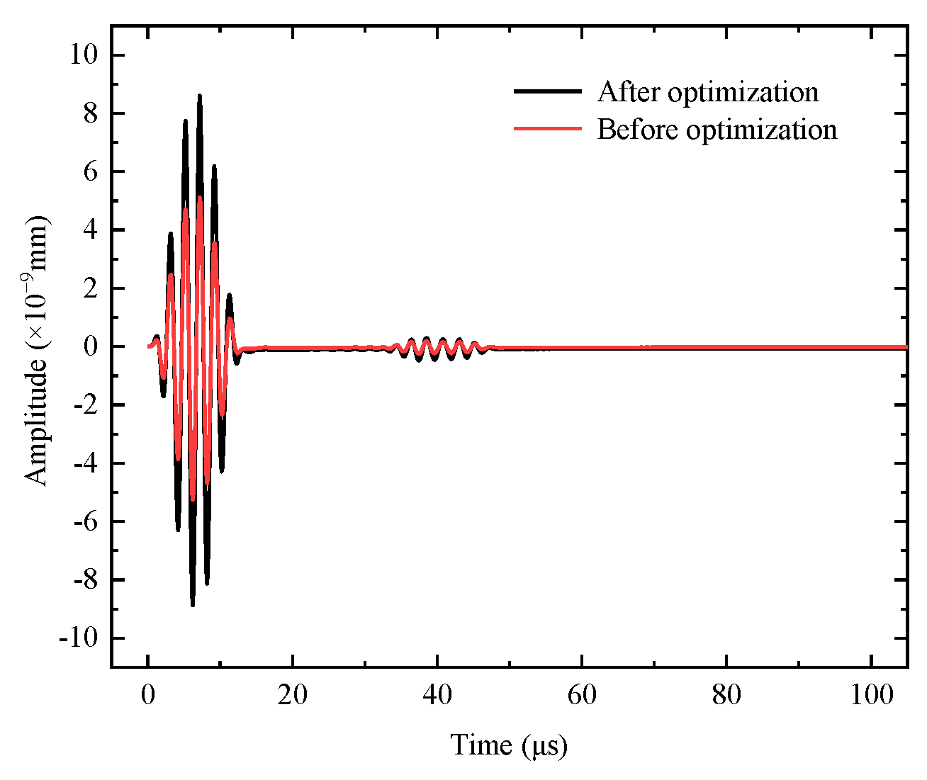
This study proposes EMUS surface wave detection of metal sheet defects aiming at improving the efficiency of the EMUS transducer, accuracy of the corresponding relation between ultrasonic signals and defect features, and measurement accuracy of the time delay between EMUS packets using an aluminum plate. The electromagnetic field distribution of the EMUS transducer, the propagation depth of the surface wave, and the influence of the grid accuracy on the EMUS excitation signal are analyzed; the orthogonal experimental design is used to optimize the excitation parameters of the EMUS surface wave transducer; the peak-to-peak value and PSD of the EMUS signal in defect detection are compared; a method for measuring the time delay of the EMUS signal wave packet is proposed; and the maximum value method and the cross-correlation method are compared. The following conclusions are drawn.

After optimizing the excitation parameters of the EMUS transducer through the orthogonal experiment design, the amplitude of the EMUS signal generated is increased by about 80%.

Using the PSD of the EMUS response signal to detect defects, the accuracy is higher than the peak-to-peak value detection, and the reliability is better; the measurement accuracy of the proposed "center zero-point method" for the EMUS signal wave packet time delay is higher than that of the peak-to-peak method and the starting point method, and the accuracy is close to that of the cross-correlation method. Certainly the boundary condition of this method should be further investigated and validated with experiments.