
Estimation of Floor Response Spectra for Self-Centering Structural Systems with Flag-Shaped Hysteretic Behavior


Abstract
:1. Introduction
2. Self-Centering (SC) SDOF System with Flag-Shaped Hysteretic Behavior, Ground Motion Records, and Numerical Modeling
3. Floor Response Spectra and Dynamic Amplification Factor from Nonlinear Response History Analysis (NLRHA)
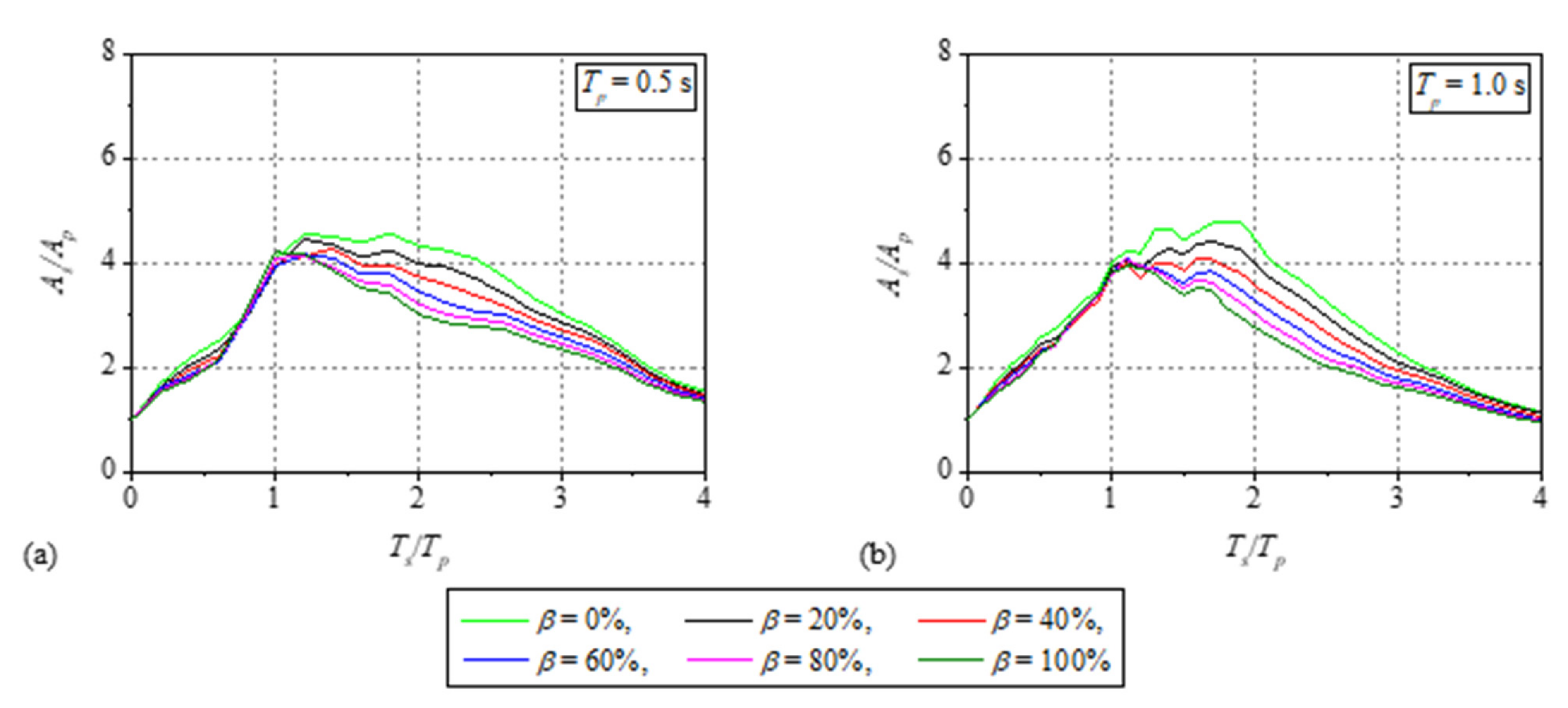
3.1. Floor Response Spectra
- (a)
- The NLRHA of the prescribed self-centering (SC) SDOF system with flag-shaped hysteretic behavior (primary structure), for the set of ground motion records and determination of the total floor acceleration response history for each ground motion record. Here, the total floor acceleration response history is the sum of the floor acceleration response history relative to the ground and the ground acceleration response history.
- (b)
- Linear RHA of the elastic SDOF system (secondary structure), using the set of total floor acceleration response histories determined from step (a), to generate floor response spectra.
- (c)
- Calculation of the mean floor response spectrum.
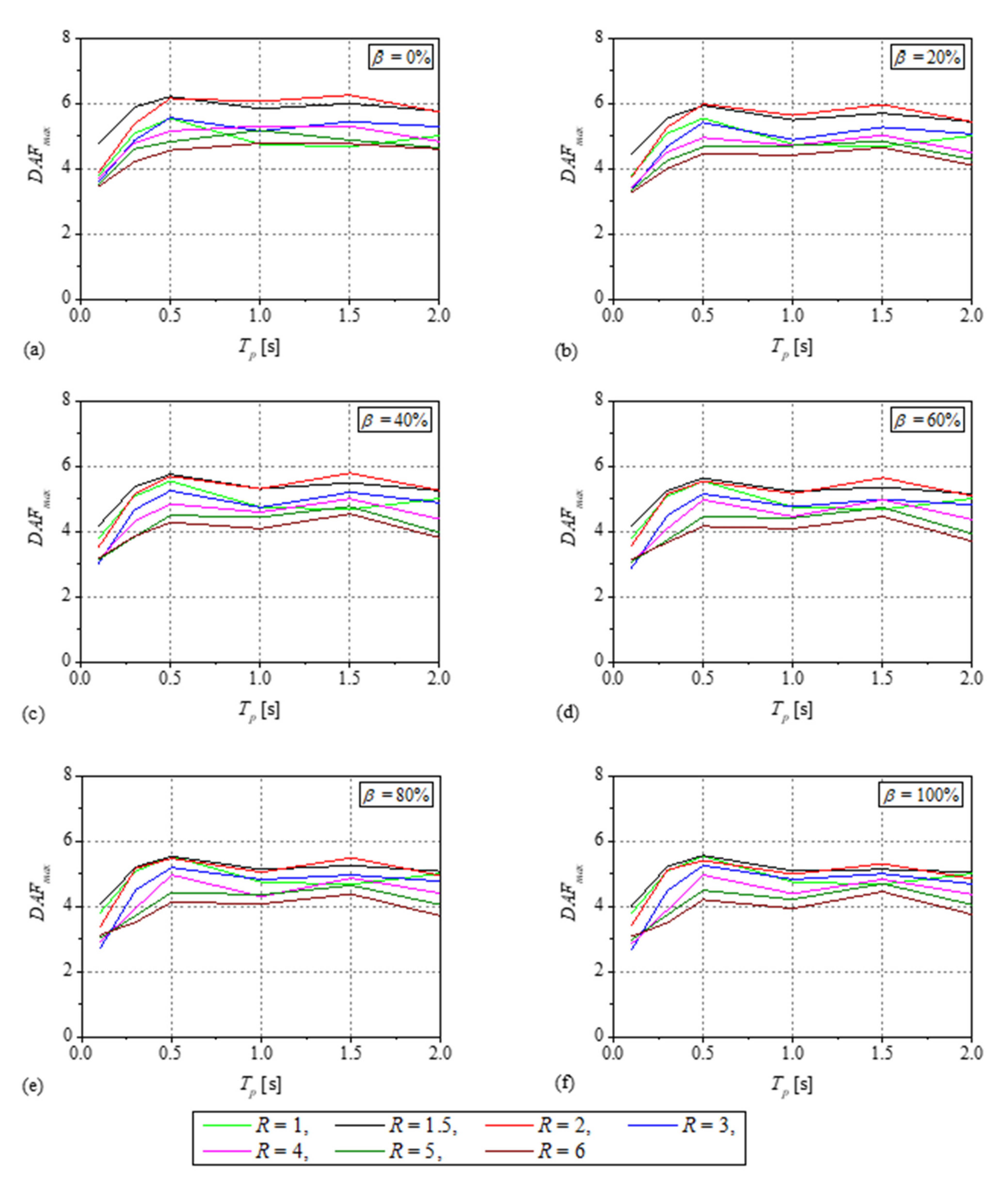
3.2. Maximum Dynamic Amplification Factor
3.3. Post-Resonance Dynamic Amplification Factor
4. Equation to Estimate Floor Response Spectra and Verification
4.1. Equation to Estimate FRS
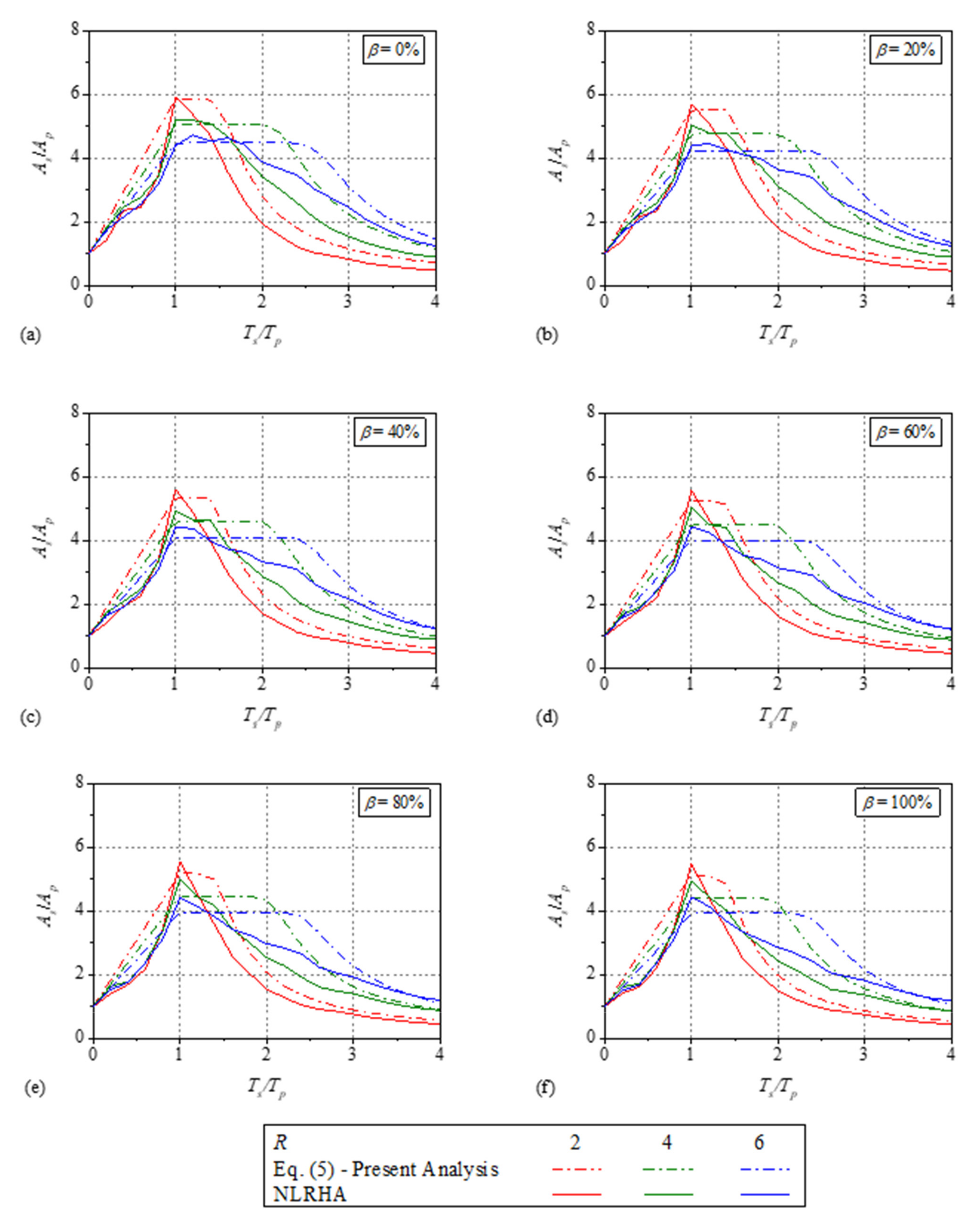
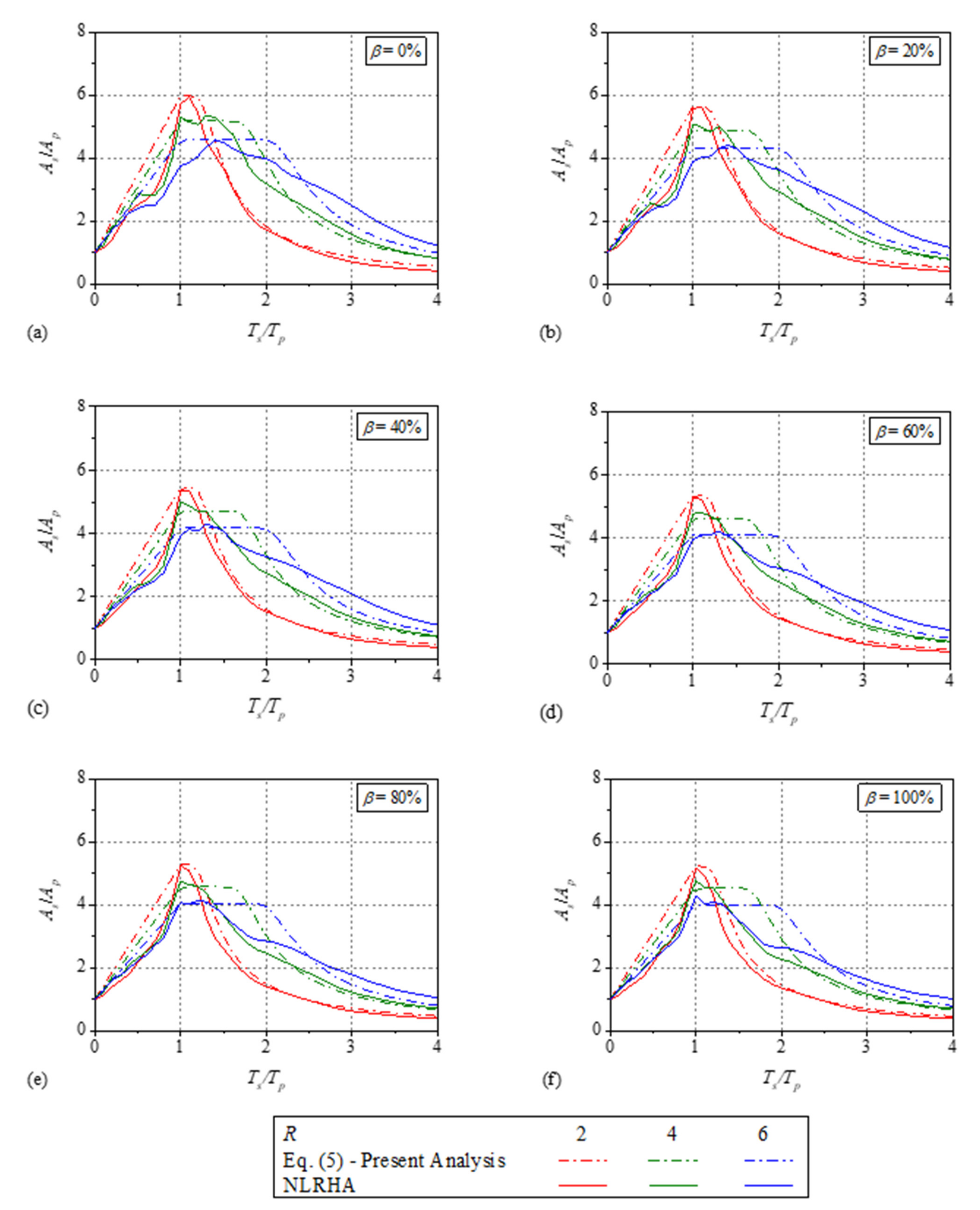
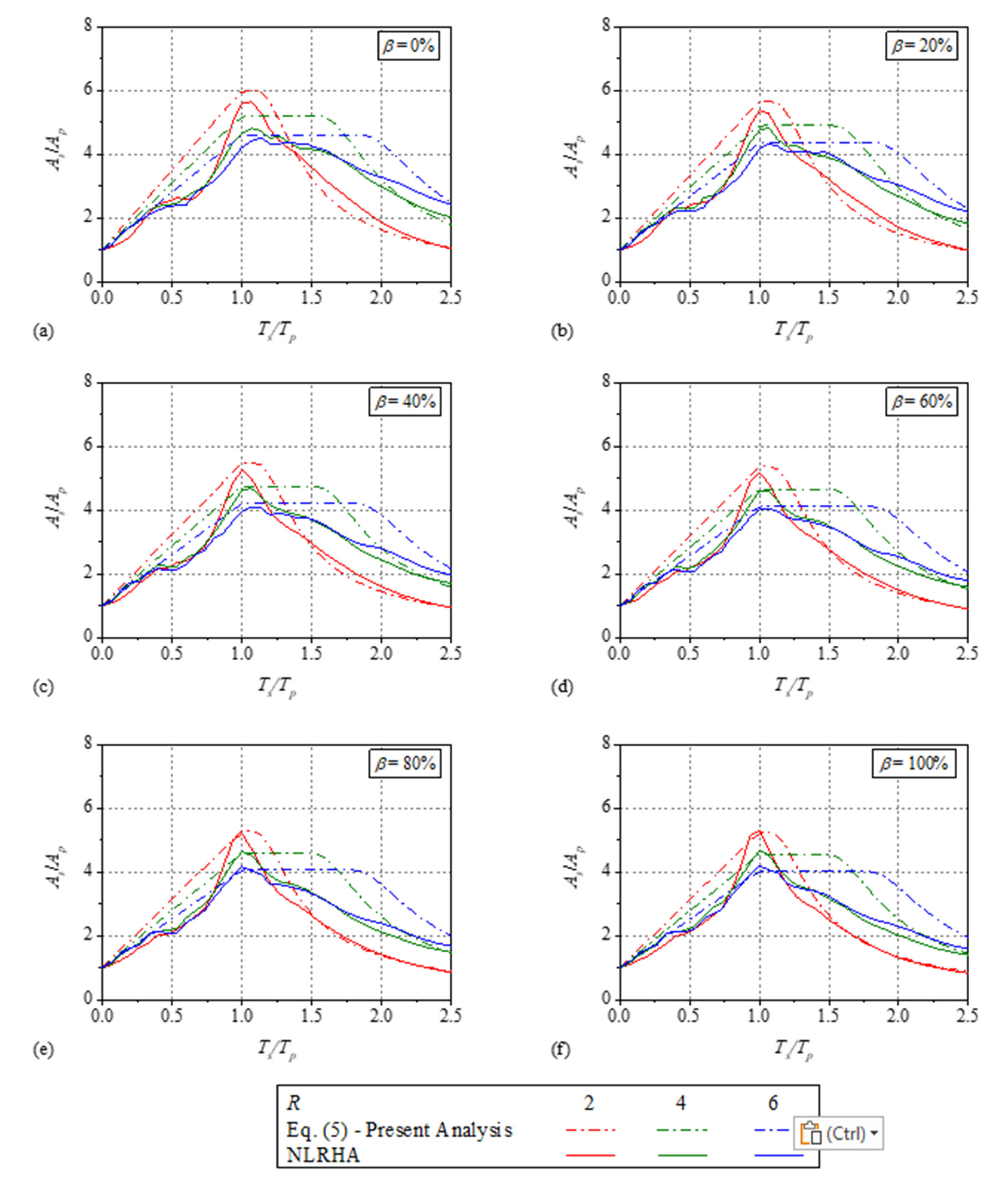
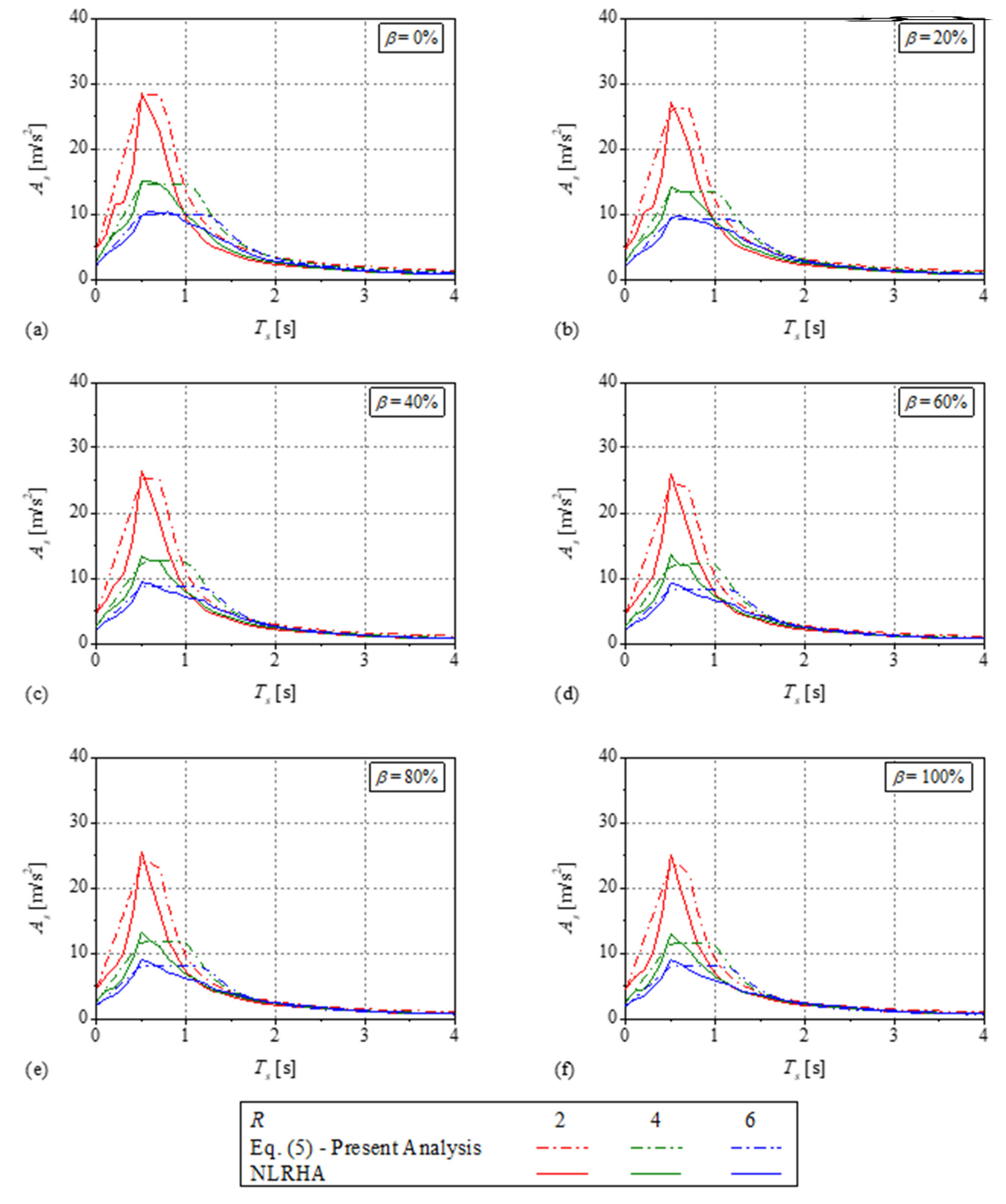
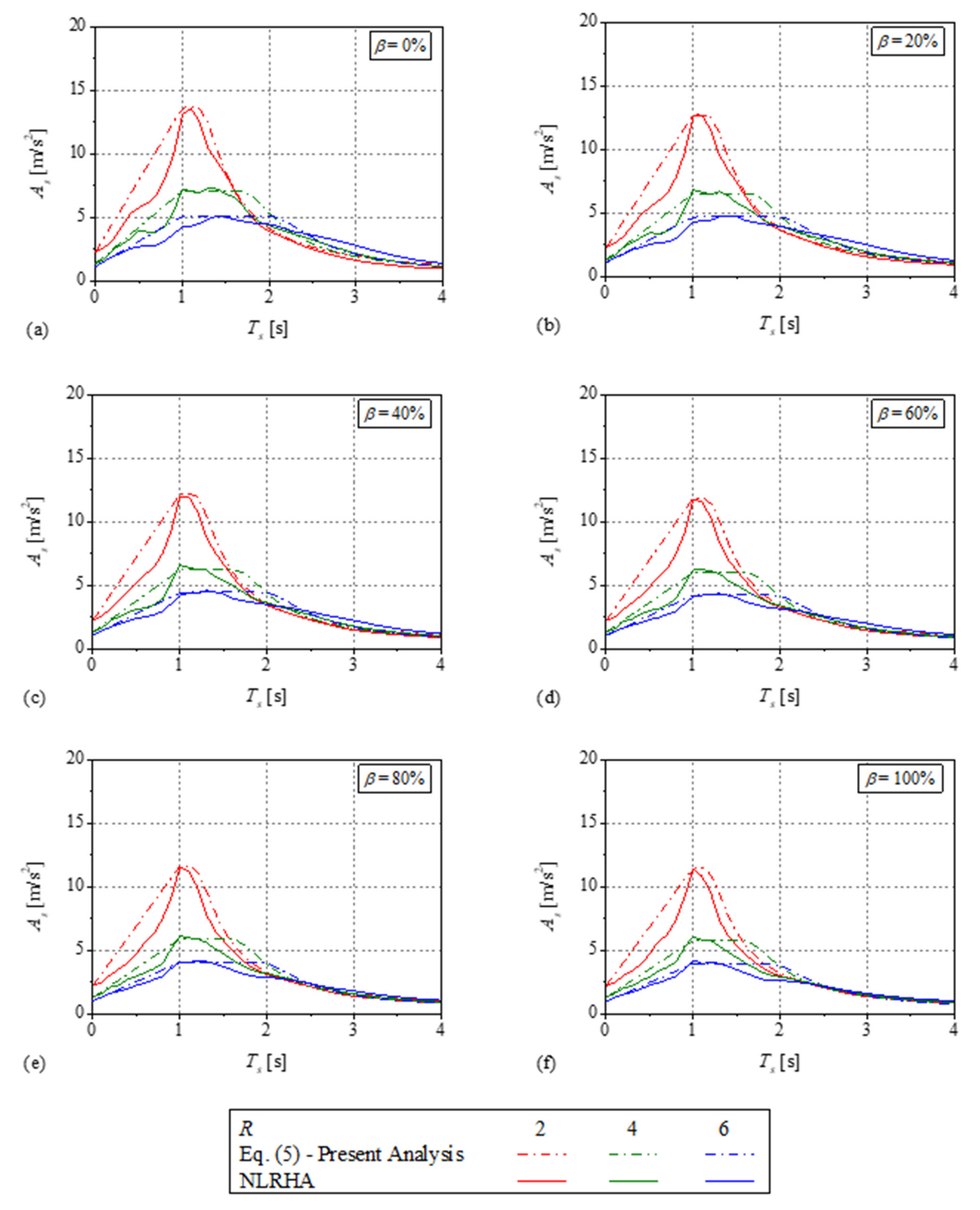
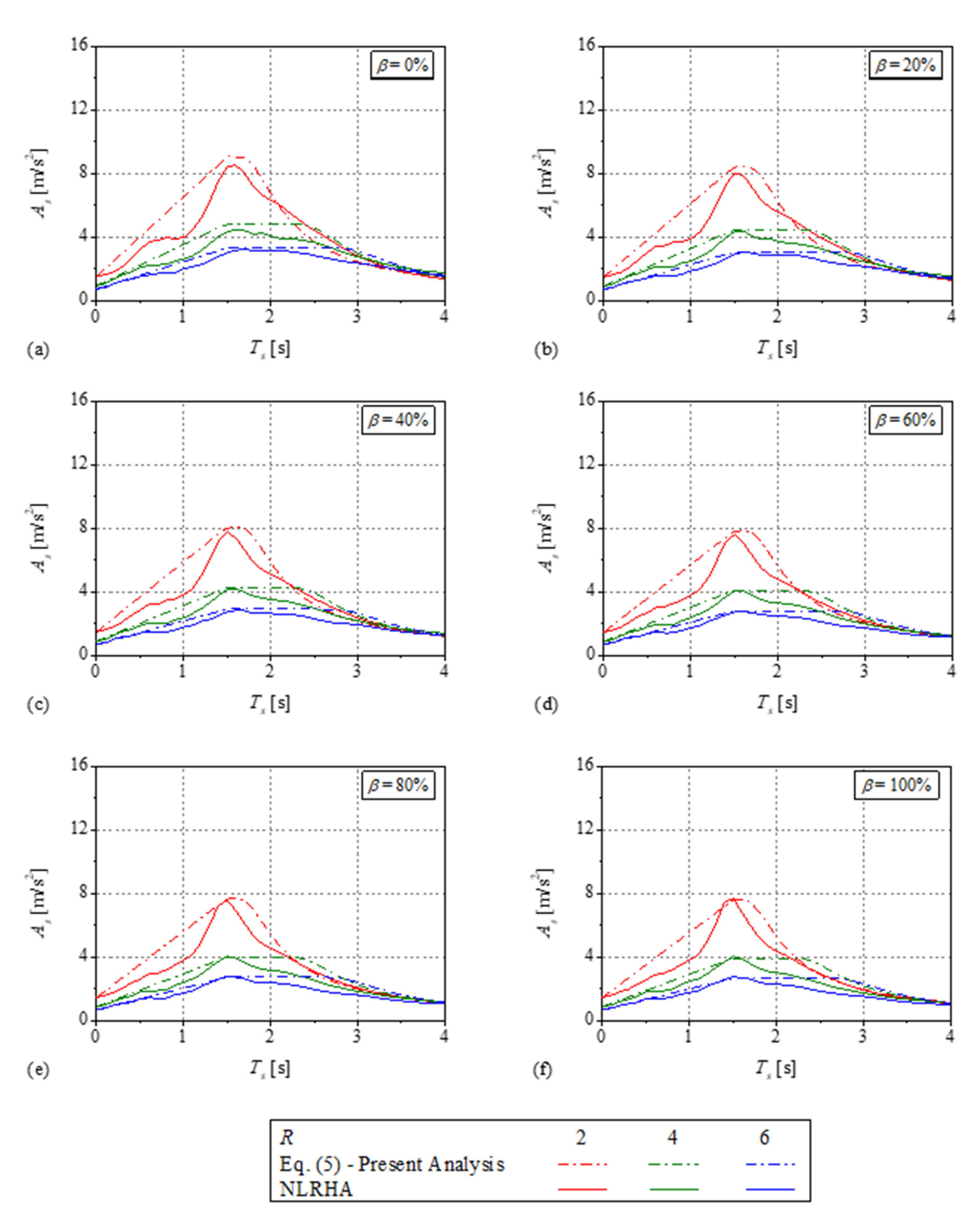
4.2. Verification of Proposed Equation to Estimate FRS
4.3. Comparison of the Proposed FRS with Existing Direct Methods
5. Conclusions
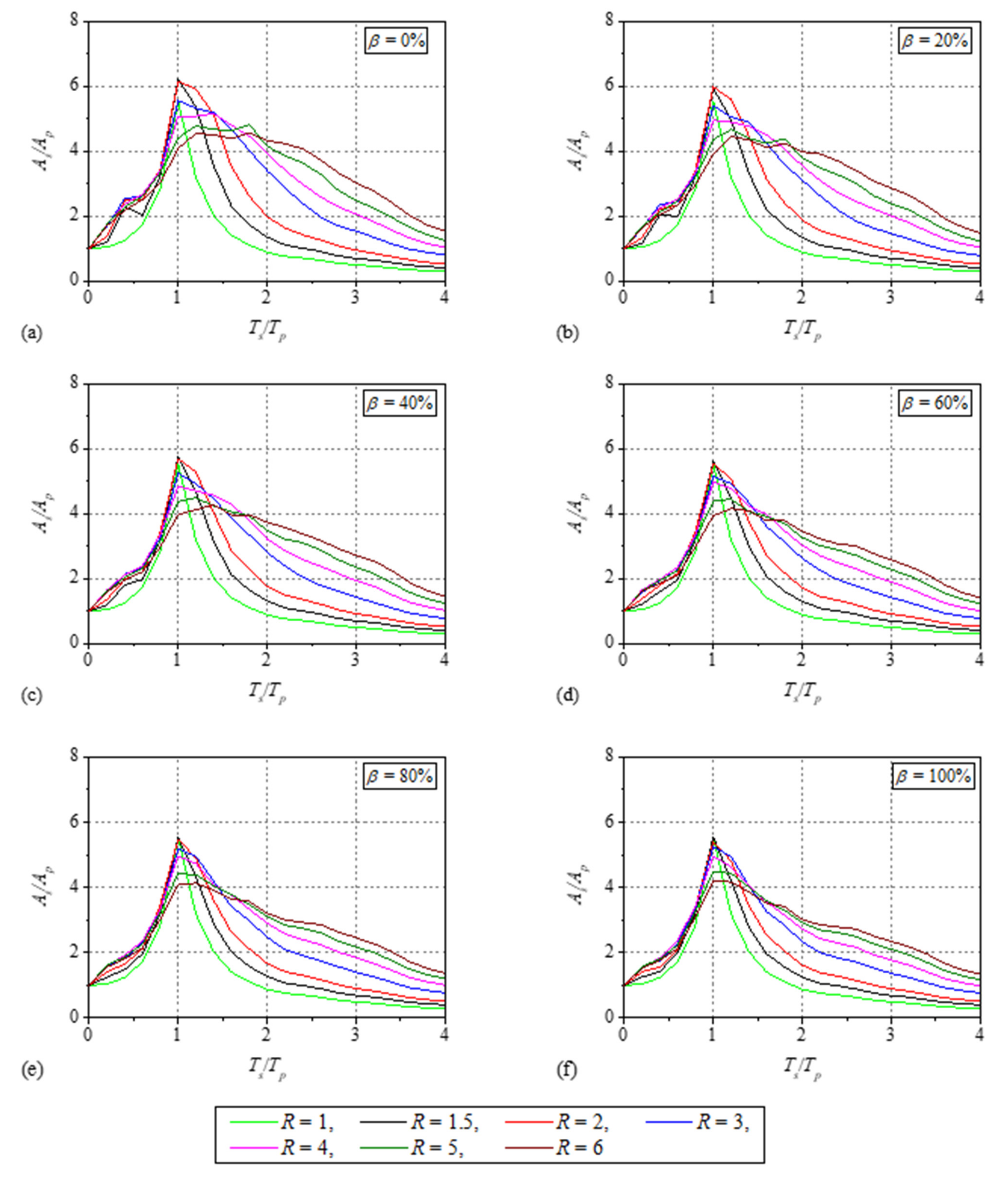
- The effect of the primary structure initial vibration period , response reduction factor , and energy dissipation parameter on the FRS is studied. A single peak was observed on the mean normalized FRS for , but for , the maximum value of the mean normalized FRS is nearly constant over a wide period range and forms a spectral plateau. The width of the spectral plateau increases with increase in and decrease in , which is due to the higher ductility demand on the primary structure. In addition, the peak value of mean normalized FRS increases when changes from 1 to 2 and then decreases for . The reduction in the mean normalized FRS was observed with increase in . With increase in , the maximum dynamic amplification factor , increases for , and remains nearly constant for and .
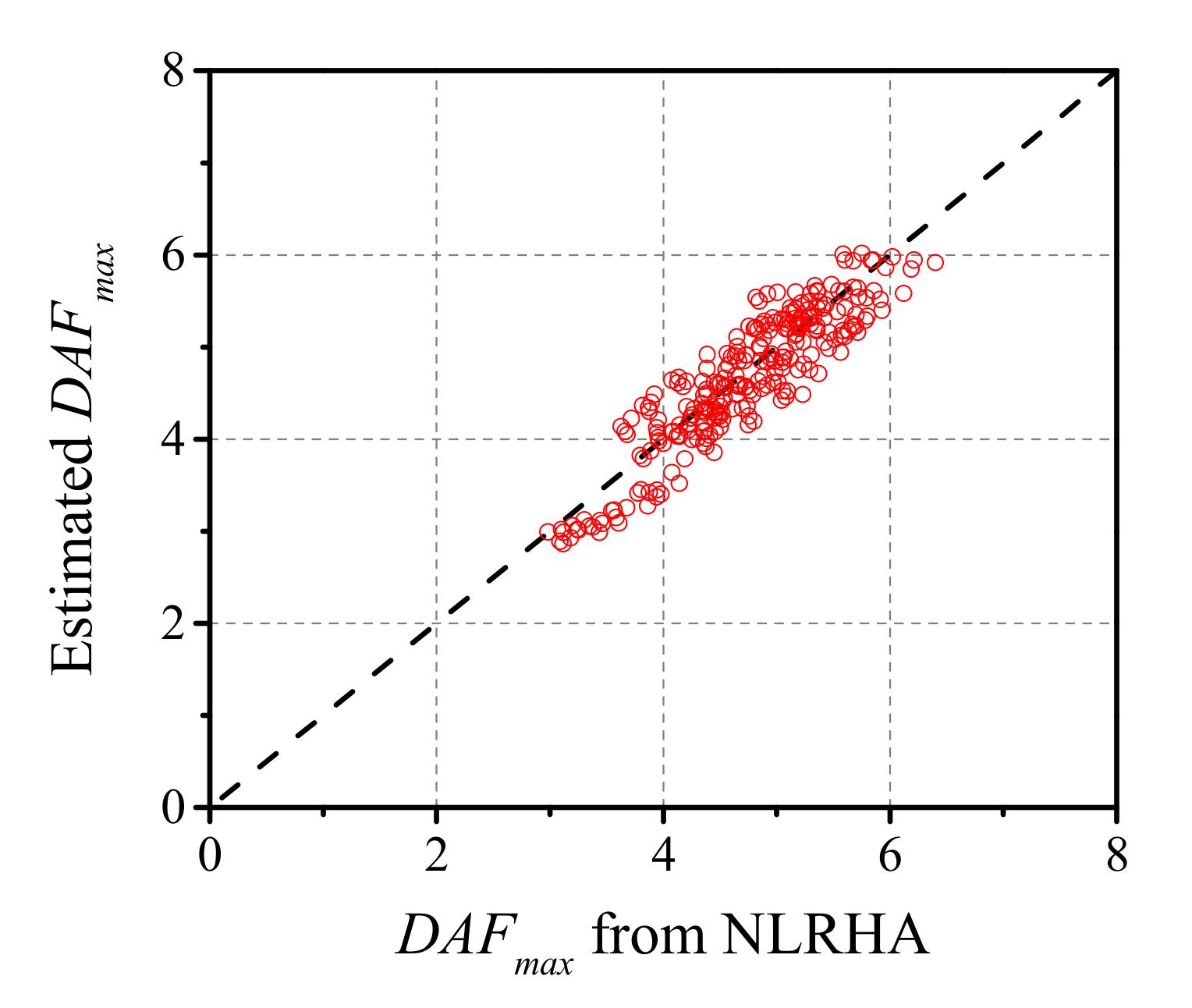
- An empirical equation for which can be used to estimate the acceleration demand in the resonance region is developed. This equation showed good accuracy when compared with NLRHA results. In addition for the post-resonance region, an equation to estimate the dynamic amplification factor is also obtained.
- An equation to estimate the FRS for SC systems with flag-shaped hysteretic behavior is proposed using the and the . The equation to estimate FRS is then validated using a different set of far-fault ground motions. It was observed that the equation to estimate FRS for SC systems with flag-shaped hysteretic behavior showed good accuracy when compared with the NLRHA results.
Author Contributions
Funding
Institutional Review Board Statement
Informed Consent Statement
Data Availability Statement
Acknowledgments
Conflicts of Interest
Appendix A. Comparison of the Normalized Floor Response Spectra
Appendix B. Existing Direct Methods to Estimate the FRS
- (a)
- In the pre- and post-resonance region,where is the value at the specific period and damping ratio in the elastic acceleration spectrum of the ground motion.
- (b)
- In the resonance region,where is the characteristic period of the ground motion.
References
- EERI. Nonstructural Issues of Seismic Design and Construction; Earthquake Engineering Research Institute: Berkeley, CA, USA, 1984. [Google Scholar]
- Villaverde, R. Seismic design of secondary structures: State of the art. J. Struct. Eng. (ASCE) 1997, 123, 1011–1019. [Google Scholar] [CrossRef]
- Dhakal R., P.; Pourali, A.; Tasligedik A., S.; Yeow, T.; Baird, A.; MacRae, G.; Pampanin, S.; Palermo, A. Seismic performance of non-structural components and contents in buildings: An overview of NZ research. Earthq. Eng. Eng. Vib. 2016, 15, 1–17. [Google Scholar] [CrossRef]
- Devin, A.; Fanning, P.J. Non-structural elements and the dynamic response of buildings: A review. Eng. Struct. 2019, 187, 242–250. [Google Scholar] [CrossRef]
- Wang, T.; Shang, Q.; Li, J. Seismic force demands on acceleration-sensitive nonstructural components: A state-of-the-art review. Earthq. Eng. Eng. Vib. 2021, 20, 39–62. [Google Scholar] [CrossRef]
- CEN. Eurocode 8: Design of Structures for Earthquake Resistance—Part 1: General Rules, Seismic Actions and Rules for Buildings (EN 1988-1); European Committee for Standardization: Brussels, Belgium, 2004. [Google Scholar]
- ASCE 7-16. Minimum Design Loads for Buildings and Other Structures; American Society of Civil Engineers (ASCE): Reston, VA, USA, 2017. [Google Scholar]
- Sullivan, T.J.; Calvi, P.M.; Nascimbene, R. Towards improved floor spectra estimates for seismic design. Earthq. Struct. 2013, 4, 109–132. [Google Scholar] [CrossRef]
- Vukobratović, V.; Fajfar, P. Code-oriented floor acceleration spectra for building structures. Bull. Earthq. Eng. 2017, 15, 3013–3026. [Google Scholar] [CrossRef]
- Aragaw, L.F.; Calvi, P.M. Earthquake-induced floor accelerations in base-rocking wall buildings. J. Earthq. Eng. 2021, 25, 941–969. [Google Scholar] [CrossRef]
- Kazantzi, A.K.; Vamvatsikos, D.; Miranda, E. The effect of damping on floor spectral accelerations as inferred from instrumented buildings. Bull. Earthq. Eng. 2020, 18, 2149–2164. [Google Scholar] [CrossRef]
- Vukobratović, V.; Yeow, T.Z.; Kusunoki, K. Floor acceleration demands in three RC buildings subjected to multiple excitations during shake table tests. Bull. Earthq. Eng. 2021, 19, 5495–5523. [Google Scholar] [CrossRef]
- Oropeza, M.; Favez, P.; Lestuzzi, P. Seismic response of nonstructural components in case of nonlinear structures based on floor response spectra method. Bull. Earthq. Eng. 2010, 8, 387–400. [Google Scholar] [CrossRef] [Green Version]
- Vukobratović, V.; Fajfar, P. A method for the direct determination of approximate floor response spectra for SDOF inelastic structures. Bull. Earthq. Eng. 2015, 13, 1405–1424. [Google Scholar] [CrossRef]
- Yasui, Y.; Yoshihara, J.; Takeda, T.; Miyamoto, A. Direct generation method for floor response spectra. In Proceedings of the Transactions of the 12th International Conference on Structural Mechanics in Reactor Technology, Stuttgart, Germany, 15–20 August 1993. [Google Scholar]
- Welch, D.P.; Sullivan, T.J. Illustrating a new possibility for the estimation of floor spectra in nonlinear multi-degree of freedom systems. In Proceedings of the 16th World Conference on Earthquake Engineering, Santiago, Chile, 9–13 January 2017. [Google Scholar]
- Calvi, P.M.; Sullivan, T.J. Estimating floor spectra in multiple degree of freedom systems. Earthq. Struct. 2014, 7, 17–38. [Google Scholar] [CrossRef]
- Vukobratović, V.; Fajfar, P. A method for the direct estimation of floor acceleration spectra for elastic and inelastic MDOF structures. Earthq. Eng. Struct. Dyn. 2016, 45, 2495–2511. [Google Scholar] [CrossRef]
- Merino R., J.; Perrone, D.; Filiatrault, A. Consistent floor response spectra for performance-based design of nonstructural elements. Earthq. Eng. Struct. Dyn. 2020, 49, 261–284. [Google Scholar] [CrossRef]
- Vukobratović, V.; Ruggieri, S. Floor acceleration demands in a twelve-storey RC shear wall building. Buildings 2021, 11, 38. [Google Scholar] [CrossRef]
- Kurama, Y.C. Hybrid post-tensioned precast concrete walls for use in seismic regions. PCI Journal 2002, 47, 36–59. [Google Scholar] [CrossRef]
- Smith, B.J.; Kurama Y., C.; McGinnis, M.J. Behavior of precast concrete shear walls for seismic regions: Comparison of hybrid and emulative specimens. J. Struct. Eng. (ASCE) 2013, 139, 1917–1927. [Google Scholar] [CrossRef] [Green Version]
- Belleri, A.; Schoettler, M.J.; Restrepo, J.I.; Fleishman, R.B. Dynamic behavior of rocking and hybrid cantilever walls in a precast concrete building. ACI Struct. J. 2014, 111, 661–672. [Google Scholar] [CrossRef]
- Buddika, H.A.D.S.; Wijeyewickrema, A.C. Seismic performance evaluation of posttensioned hybrid precast wall-frame buildings and comparison with shear wall-frame buildings. J. Struct. Eng. (ASCE) 2016, 142, 04016021. [Google Scholar] [CrossRef]
- Shrestha, B.K.; Wijeyewickrema, A.C.; Kono, S. Seismic performance and collapse safety assessment of post-tensioned hybrid precast concrete infill wall-frames and comparison with reinforced concrete infill wall-frames. J. Earthq. Eng. 2021; 1–24, in press. [Google Scholar] [CrossRef]
- Priestley, M.J.N.; Calvi, G.M.; Kowalsky, M.J. Displacement-Based Seismic Design of Structures; IUSS Press: Pavia, Italy, 2007. [Google Scholar]
- Yang, B.; Lu, X. Displacement-based seismic design approach for prestressed precast concrete shear walls and its application. J. Earthq. Eng. 2018, 22, 1836–1860. [Google Scholar] [CrossRef]
- Rahgozar, N.; Moghadam, A.S.; Aziminejad, A. Inelastic displacement ratios of fully self-centering controlled rocking systems subjected to near-source pulse-like ground motions. Eng. Struct. 2016, 108, 113–133. [Google Scholar] [CrossRef]
- Zhang, C.; Steele, T.C.; Wiebe, L.D.A. Design-level estimation of seismic displacements for self-centering SDOF systems on stiff soil. Eng. Struct. 2018, 177, 431–443. [Google Scholar] [CrossRef]
- Dong, H.; Han, Q.; Du, X.; Liu, J. Constant ductility inelastic displacement ratios for the design of self-centering structures with flag-shaped model subjected to pulse-type ground motions. Soil Dyn. Earthq. Eng. 2020, 133, 106143. [Google Scholar] [CrossRef]
- FEMA P695. Quantification of Building Seismic Performance Factors; Federal Emergency Management Agency (FEMA): Washington, DC, USA, 2009. [Google Scholar]
- OpenSees. OpenSees. Open system for earthquake engineering simulation. In Computer Program; University of California: Berkeley, CA, USA, 2017; Available online: https://opensees.berkeley.edu/ (accessed on 1 April 2017).
- Bates, D.M.; Watts, D.G. Nonlinear Regression Analysis and Its Applications; Wiley: New York, NY, USA, 1988. [Google Scholar]
- SPSS. IBM SPSS Statistics for Windows; Version 25.0; IBM Corp.: Armonk, NY, USA, 2017. [Google Scholar]


| EQ. No. | Event | Year | Station | Fault Type |
PGA Component 1 |
PGA Component 2 | (m/s) | ||
|---|---|---|---|---|---|---|---|---|---|
| 1 | Northridge | 1994 | Beverly Hills - Mulhol | Thrust | 6.7 | 17.2 | 0.42 | 0.52 | 356 |
| 2 | Northridge | 1994 | Canyon Country-WLC | Thrust | 6.7 | 12.4 | 0.41 | 0.48 | 309 |
| 3 | Duzce, Turkey | 1999 | Bolu | Strike-slip | 7.1 | 12.0 | 0.73 | 0.82 | 326 |
| 4 | Hector Mine | 1999 | Hector | Strike-slip | 7.1 | 11.7 | 0.27 | 0.34 | 685 |
| 5 | Imperial Valley | 1979 | Delta | Strike-slip | 6.5 | 22.0 | 0.24 | 0.35 | 275 |
| 6 | Imperial Valley | 1979 | El Centro Array #11 | Strike-slip | 6.5 | 12.5 | 0.36 | 0.38 | 196 |
| 7 | Kobe, Japan | 1995 | Nishi-Akashi | Strike-slip | 6.9 | 7.1 | 0.51 | 0.50 | 609 |
| 8 | Kobe, Japan | 1995 | Shin-Osaka | Strike-slip | 6.9 | 19.2 | 0.24 | 0.21 | 256 |
| 9 | Kocaeli, Turkey | 1999 | Duzce | Strike-slip | 7.5 | 15.4 | 0.31 | 0.36 | 276 |
| 10 | Kocaeli, Turkey | 1999 | Arcelik | Strike-slip | 7.5 | 13.5 | 0.22 | 0.15 | 523 |
| 11 | Landers | 1992 | Yermo Fire Station | Strike-slip | 7.3 | 23.6 | 0.24 | 0.15 | 354 |
| Coefficients | |||||||
|---|---|---|---|---|---|---|---|
| −0.020 | −0.001 | −0.013 | −0.021 | −0.017 | −0.019 | −0.018 | |
| −1.304 | −2.358 | −1.574 | −1.400 | −1.382 | −1.258 | −1.178 | |
| 1.259 | 1.330 | 1.350 | 1.260 | 1.175 | 1.108 | 1.043 |
|
EQ No. | Event | Year | Station | Fault Type | PGA Component 1 | PGA Compontent 2 | (m/s) | ||
|---|---|---|---|---|---|---|---|---|---|
| 1 | Landers | 1992 | Coolwater | Strike-slitd | 7.3 | 19.7 | 0.28 | 0.42 | 271 |
| 2 | Loma tdrieta | 1989 | Capitola | Strike-slip | 6.9 | 15.2 | 0.53 | 0.44 | 289 |
| 3 | Loma Prieta | 1989 | Gilroy Array #3 | Strike-slip | 6.9 | 12.8 | 0.56 | 0.37 | 350 |
| 4 | Manjil, Iran | 1990 | Abbar | Strike-slip | 7.4 | 12.6 | 0.51 | 0.50 | 724 |
| 5 | Superstition Hills | 1987 | El Centro Imp. Co. | Strike-slip | 6.5 | 18.2 | 0.36 | 0.26 | 192 |
| 6 | Superstition Hills | 1987 | Poe Road (temp) | Strike-slip | 6.5 | 11.2 | 0.45 | 0.30 | 208 |
| 7 | Catde Mendocino | 1992 | Rio Dell Overpass | Thrust | 7.0 | 14.3 | 0.39 | 0.55 | 312 |
| 8 | Chi-Chi, Taiwan | 1999 | CHY101 | Thrust | 7.6 | 10.0 | 0.35 | 0.44 | 259 |
| 9 | Chi-Chi, Taiwan | 1999 | TCU045 | Thrust | 7.6 | 26.0 | 0.47 | 0.51 | 705 |
| 10 | San Fernando | 1971 | LA - Hollywood Stor | Thrust | 6.6 | 22.8 | 0.21 | 0.17 | 316 |
| 11 | Friuli, Italy | 1976 | Tolmezzo | Thrust | 6.5 | 15.8 | 0.35 | 0.31 | 425 |
Publisher’s Note: MDPI stays neutral with regard to jurisdictional claims in published maps and institutional affiliations. |
© 2022 by the authors. Licensee MDPI, Basel, Switzerland. This article is an open access article distributed under the terms and conditions of the Creative Commons Attribution (CC BY) license (https://creativecommons.org/licenses/by/4.0/).
Share and Cite
Shrestha, B.K.; Wijeyewickrema, A.C.; Miyashita, H.; Malla, N. Estimation of Floor Response Spectra for Self-Centering Structural Systems with Flag-Shaped Hysteretic Behavior. Buildings 2022, 12, 167. https://doi.org/10.3390/buildings12020167
Shrestha BK, Wijeyewickrema AC, Miyashita H, Malla N. Estimation of Floor Response Spectra for Self-Centering Structural Systems with Flag-Shaped Hysteretic Behavior. Buildings. 2022; 12(2):167. https://doi.org/10.3390/buildings12020167
Chicago/Turabian StyleShrestha, Binod Kumar, Anil C. Wijeyewickrema, Hiroki Miyashita, and Niraj Malla. 2022. "Estimation of Floor Response Spectra for Self-Centering Structural Systems with Flag-Shaped Hysteretic Behavior" Buildings 12, no. 2: 167. https://doi.org/10.3390/buildings12020167
APA StyleShrestha, B. K., Wijeyewickrema, A. C., Miyashita, H., & Malla, N. (2022). Estimation of Floor Response Spectra for Self-Centering Structural Systems with Flag-Shaped Hysteretic Behavior. Buildings, 12(2), 167. https://doi.org/10.3390/buildings12020167