Civil Infrastructure Damage and Corrosion Detection: An Application of Machine Learning

Abstract

Automatic detection of corrosion and associated damages to civil infrastructures such as bridges, buildings, and roads, from aerial images captured by an Unmanned Aerial Vehicle (UAV), helps one to overcome the challenges and shortcomings (objectivity and reliability) associated with the manual inspection methods. Deep learning methods have been widely reported in the literature for civil infrastructure corrosion detection. Among them, convolutional neural networks (CNNs) display promising applicability for the automatic detection of image features less affected by image noises. Therefore, in the current study, we propose a modified version of deep hierarchical CNN architecture, based on 16 convolution layers and cycle generative adversarial network (CycleGAN), to predict pixel-wise segmentation in an end-to-end manner using the images of Bolte Bridge and sky rail areas in Victoria (Melbourne). The convolutedly designed model network proposed in the study is based on learning and aggregation of multi-scale and multilevel features while moving from the low convolutional layers to the high-level layers, thus reducing the consistency loss in images due to the inclusion of CycleGAN. The standard approaches only use the last convolutional layer, but our proposed architecture differs from these approaches and uses multiple layers. Moreover, we have used guided filtering and Conditional Random Fields (CRFs) methods to refine the prediction results. Additionally, the effectiveness of the proposed architecture was assessed using benchmarking data of 600 images of civil infrastructure. Overall, the results show that the deep hierarchical CNN architecture based on 16 convolution layers produced advanced performances when evaluated for different methods, including the baseline, PSPNet, DeepLab, and SegNet. Overall, the extended method displayed the Global Accuracy (GA); Class Average Accuracy (CAC); mean Intersection Of the Union (IOU); Precision (P); Recall (R); and F-score values of 0.989, 0.931, 0.878, 0.849, 0.818 and 0.833, respectively.

1. Introduction and Background

Corrosion is the degradation of material properties due to environmental interactions that ultimately cause the failure of civil infrastructures [1]. Corrosion is classified into eight categories based on the morphology of the attack and the type of environment to which the structure is exposed. Uniform or general corrosion is the most dominant type of corrosion, which includes rusting of steel bridges, rusting of underground pipelines, tarnishing of silver, and patina formation on copper roofs and bronze statues [2]. The World Corrosion Organization has delineated corrosion as an extremely hazardous phenomenon that has caused significant damage to global infrastructure amounting to 2.5 trillion USD [3]. Therefore, it is one of the major defects evident in the structural materials or systems and has a considerable impact on the economy and on safety [4].

Early detection with concurrent maintenance is essential for maintaining safety and reducing the costs associated with corrosion-related damages [4,5]. Therefore, it is of extreme importance to monitor the condition and health of civil infrastructures to assure the safety of human lives and reduce the associated financial losses in line with modern smart city initiatives [6,7]. Traditionally, human-based visual inspection systems have been used to monitor the structural health of civil infrastructures [8]. However, these visual inspection methods are highly subjective, mainly due to variable personal evaluation approaches used by the involved personnel. Therefore, visual inspection of civil infrastructures such as bridges can lead to highly variable outcomes that depend on multiple factors [9]. These factors include but are not limited to the height of UAV, the field of view (FoV), camera pose, weather conditions, and photometric quantities [10]. As a result, these visual inspection systems display numerous limitations in terms of monitoring corrosion in civil infrastructures, which ultimately lead to lower overall structural reliability [11], pose threats to human lives [12], and result in a huge economic burden due to high maintenance costs.

Corrosion mainly consists of two main visual characteristics: rough texture surface and product color. Therefore, it is recommended to develop algorithms for corrosion detection, with the help of texture analysis and color analysis [9]. These two features can be applied on a stand-alone basis or implemented in a pattern recognition technique [9,10]. Furthermore, digital image processing unlocks various real-life opportunities to explore a variety of environments [11,12]. In comparison to the conventional techniques, digital image processing provides an economical, easy to handle, fast, and accurate approach to be used for large civil infrastructures such as metal bridges, tunnels, poles, and ships [13,14]. Moreover, structural monitoring of the civil infrastructures is an area that has gained considerable importance in terms of assessing the fitness and health of infrastructures. For at least half of the century, numerous structural monitoring approaches have been applied to civil infrastructures using modern sensor-based technology, including load cells, transducers, strain gauges, thermistors, accelerometer, anemometer, microphone, and internet camera technology [15,16].

However, during the last two decades, a shift has been observed to computational approaches to monitor the structural health of infrastructures [17]. The computer-based methods are designed to assist in measuring aging in infrastructures to provide timely responses to ensure safety and reduce economic losses [17]. Nowadays, the research focuses on replacing visual inspection methods with more efficient computer vision-based methods that can efficiently assess buildings, roads, bridges, and underground tunnels to identify damage-sensitive features [18]. Tian et al. [19] used computer vision to identify metal corrosion through the design of a combined Faster-Region Based Convolutional Neural Networks (Faster R-CNN) model and the Hue-Saturation-Intensity (HSI) color feature, to achieve higher correctness and recall rate. Hoang [20] has proposed a computer vision and data-driven method for detecting pitting corrosion. This method is based on history-based adaptive differential evolution with linear population size reduction (LSHADE) integrated with various image processing techniques and support vector machine (SVM) [21]. Numerous other computer-based image processing techniques have been reported to assess corrosion in civil infrastructures. For example, Pragalath et al. [22] have reported using a fuzzy logic framework combined with a recently developed image processing algorithm to measure damages to or the structural health of civil infrastructures. To address the pitting corrosion that causes serious failures to infrastructures, Hoang developed a method based on computer vision, constituting a data-driven approach [20]. Over the recent years, technological breakthroughs have been achieved in developing computer vision techniques to assess civil infrastructures. This has also increased the applicability of artificial intelligence (AI) models based on artificial neural networks (ANNs) and convolutional neural networks (CNNs). Huang et al. [23] have proposed a damage identification system in steel frames through a neural network integrated with time series and variable temperatures. Liu et al. [24] used the CNN (Faster R-CNN) architecture and a Visual Geometry Group-19 model (VGG-19 model) to quantify and assess corrosion in civil infrastructure. Atha and Jahanshahi [4] developed various CNN models for corrosion detection. Additionally, a CNN-based deep learning method for damage detection (i.e., cracks) has been reported by Munawar et al. [25]. Suh and Cha [26] used a modified version of the Faster R-CNN to evaluate and quantify multiple types of structural damages. Furthermore, Atha and Jahanshahi [4] reported using different CNN architectures to assess corrosion on metal structures. It was shown that CNNs perform better in comparison to advanced vision-based corrosion detection methods.

The advancements in machine learning and AI have also led to a greater emphasis on applying hybrid approaches that ultimately display improved accuracy and reliability [27]. Accordingly, the detection of structural corrosion from infrastructures has been demonstrated using drone images (for automated image analysis) [28]. Furthermore, an ensemble deep learning approach was used in a relevant study, displaying better efficacy than the existing approaches [29]. Furthermore, the new PAnoramic surface damage DEtection Network (PADENet) has been reported to assess corrosion from metal structures. The PADENet method is based on an unmanned aerial vehicle (UAV) for capturing panoramic images, a distorted panoramic augmentation method, the use of multiple projection techniques, a modified CNN (faster region-based), and training through transfer learning on VGG-16 [30].

The reported literature highlights the importance of image processing and machine learning over traditional corrosion detection and assessment methods in civil works [31]. Most prominently, utilizing an ImageNet Large-Scale Visual Recognition Challenge (LSVRC-2010) and deep CNNs for the training and classification of approximately 1.2 million high-resolution images has produced promising results [32]. Accordingly, numerous studies based on CNN architectures have been reported extensively in the literature [4]. Sensor-based technologies are very expensive; thus, we need a plethora of resources to deploy these sensor-based systems, and we still need a fusion-based technique to improve accuracy. Sensor-based systems are time-consuming and require extensive manual work and engineering output. Moreover, the output provided by the sensor also significantly affects the final decision.

However, a visual inspection provides a solution that lacks consistency and sustainability. On the contrary, many municipalities do not conduct infrastructure inspections appropriately and frequently due to a lack of viable methods and human resources. This situation increases the overall risk posed by deteriorating structures. Apart from visual inspection methods, modern municipalities, with enough resources, answer the problem by employing quantitative determination-based solutions, such as using a mobile measurement system (MMS) or laser-scanning. However, though quantitative inspections are accurate and consistent, they are too expensive to conduct such comprehensive inspections [33].

In the current study, we aim to develop a robust CNN-based classifier for corrosion detection on civil infrastructures such as bridges. Our proposed CNN-based methodology will be effectively used for large-scale corrosion detections as it is based on a cycle generative adversarial network (CycleGAN). The applicability of the generative adversarial network (GAN) has gained phenomenal progress in deep learning methods during recent years. It provides a novel strategy for model training using a max–min two-player game [34]. Initially, a fully connected layered generator configuration was used for GAN to generate images from random noised images. The CycleGAN provides effective training without using the pair data for image style transfer and can prevent the overfitting problem during training. Owing to the wider applicability of CycleGANs, corrosion detection on surfaces can be treated as an image-to-image translation problem. The CycleGAN is a style-changing image generation network; thus, the generated data will not differ much from the original data. Thus, this study proposes the automatic detection of corrosion with the application of CycleGAN and minimizing manual defect detection. The proposed novel methodology is effective for identifying possible cracks and corrosion. Cycle GAN has been found to enhance corrosion detection accuracy and performs much better than other traditional methods. It employs a novel compositional layer-based architecture for generating realistic defects within various image backgrounds with different textures and appearances. It can also mimic the variations of defects and offer flexible control over the locations and categories of the generated defects within the image background.

Overall, the CNN-based architecture proposed in the current study is highly efficient in detecting corrosion features with greater accuracy due to pixel-wise segmentation. Moreover, the proposed architecture will help in overcoming the processing overhead. However, besides the various advantages, the current approach displays certain limitations and challenges due to the inclusion of CycleGAN, such as instability, the collapse of mode, and non-convergence. These are due to inappropriate architectural design, objective function, and the usage of the optimization algorithm. Additionally, the one-to-one mappings used by the CycleGAN lead to a limitation where the model associates a single input image with a single output image that is not suitable for application in complex environments. Therefore, the current architecture considers manipulating the photometric values and HSV (Hue Saturation, Value) for data augmentation.

In the current study, after the introduction section, we elaborate on the detailed architecture and the methodology used for the corrosion detection of civil infrastructures such as bridge. After the methodology section, the results are elaborated in the results and discussion section using an image data set from two locations, mainly the Bolte Bridge and sky rail, Victoria as shown in Figure 1a,b. Also, the list of abbreviations used in this study is given in Abbreviations part.

2. Materials and Methods

In the methodology section, we provide the details of the dataset, followed by a discussion of the image processing procedure and the proposed scheme used for the study. The methodology of the proposed method is presented in Figure 2.

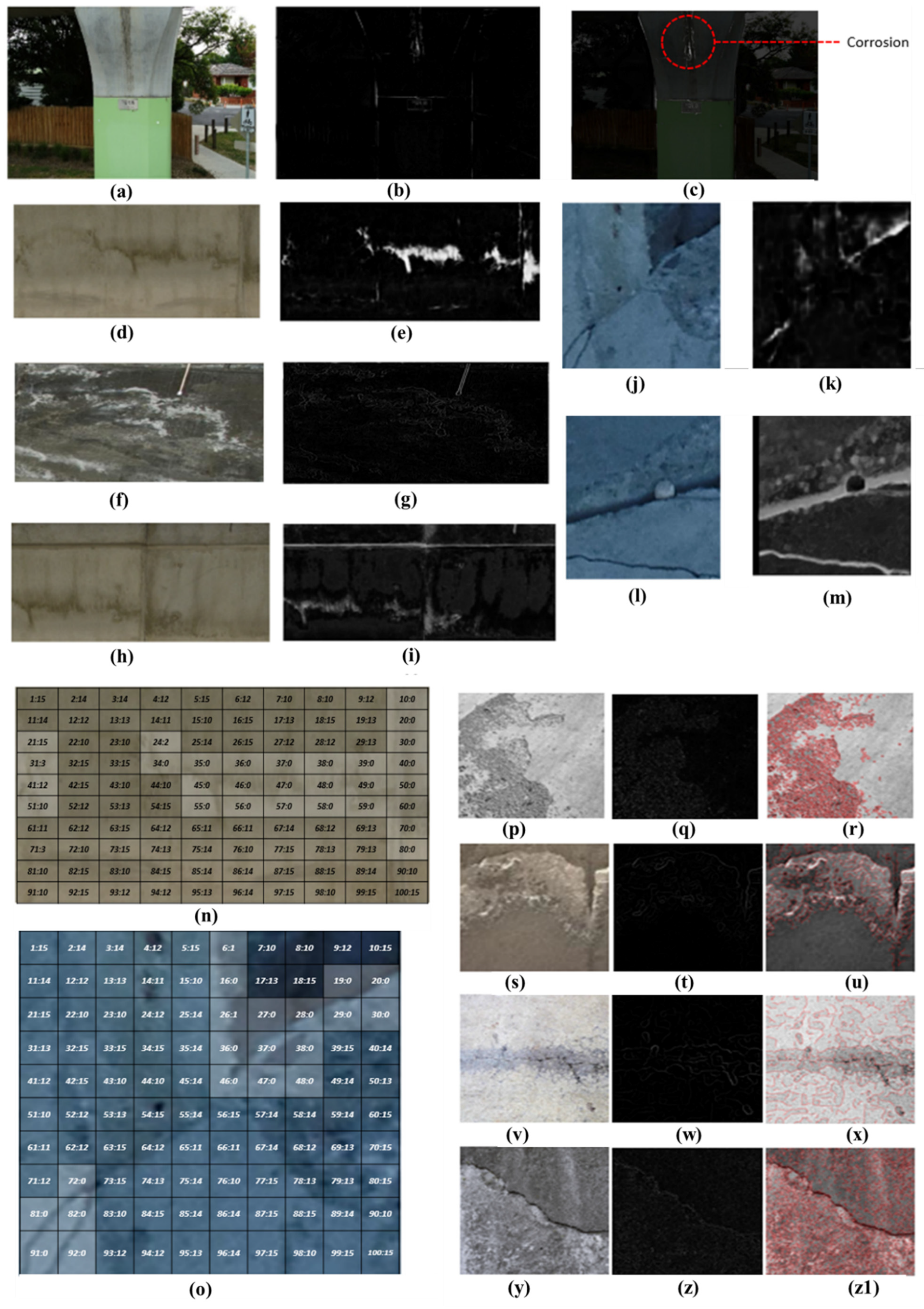
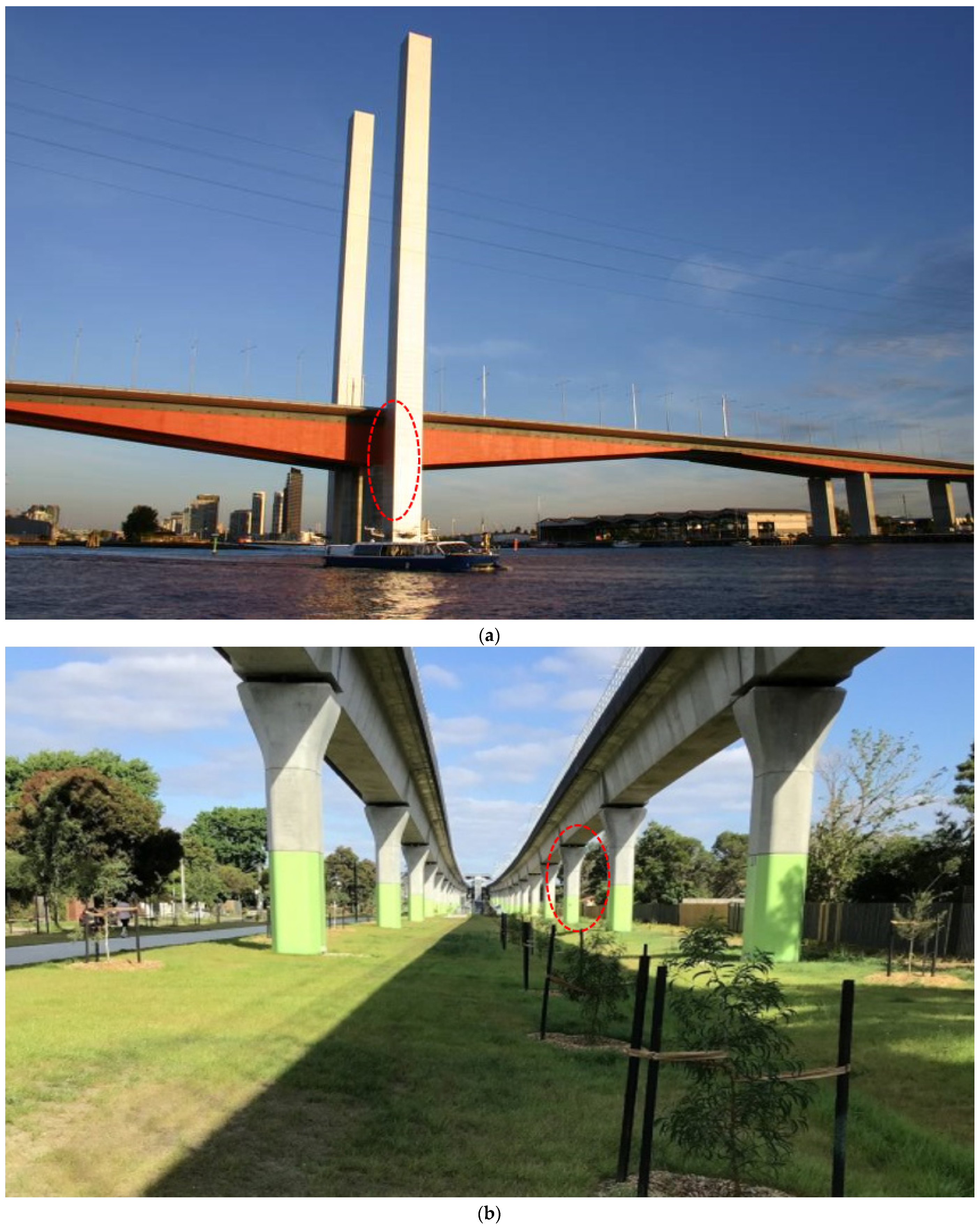
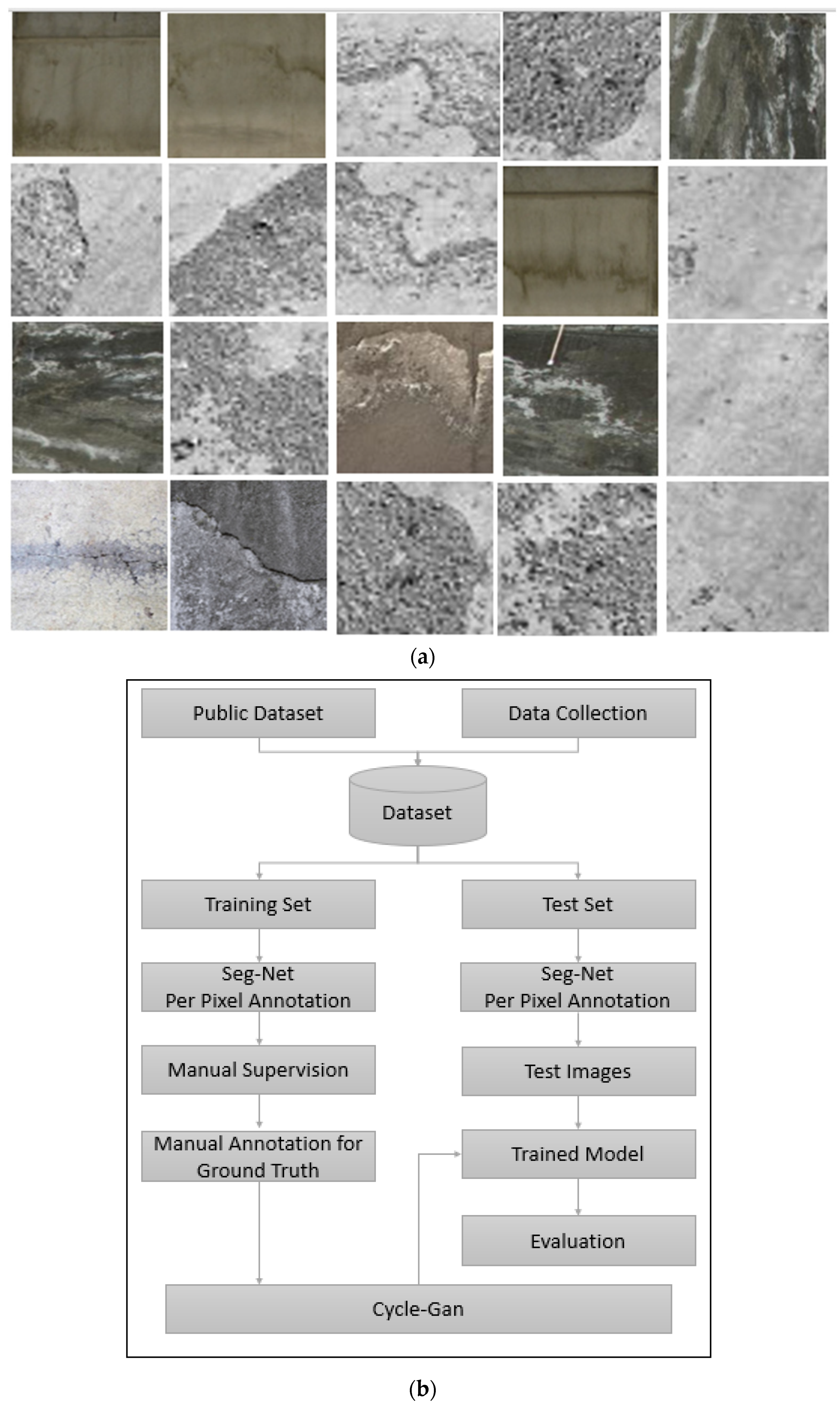
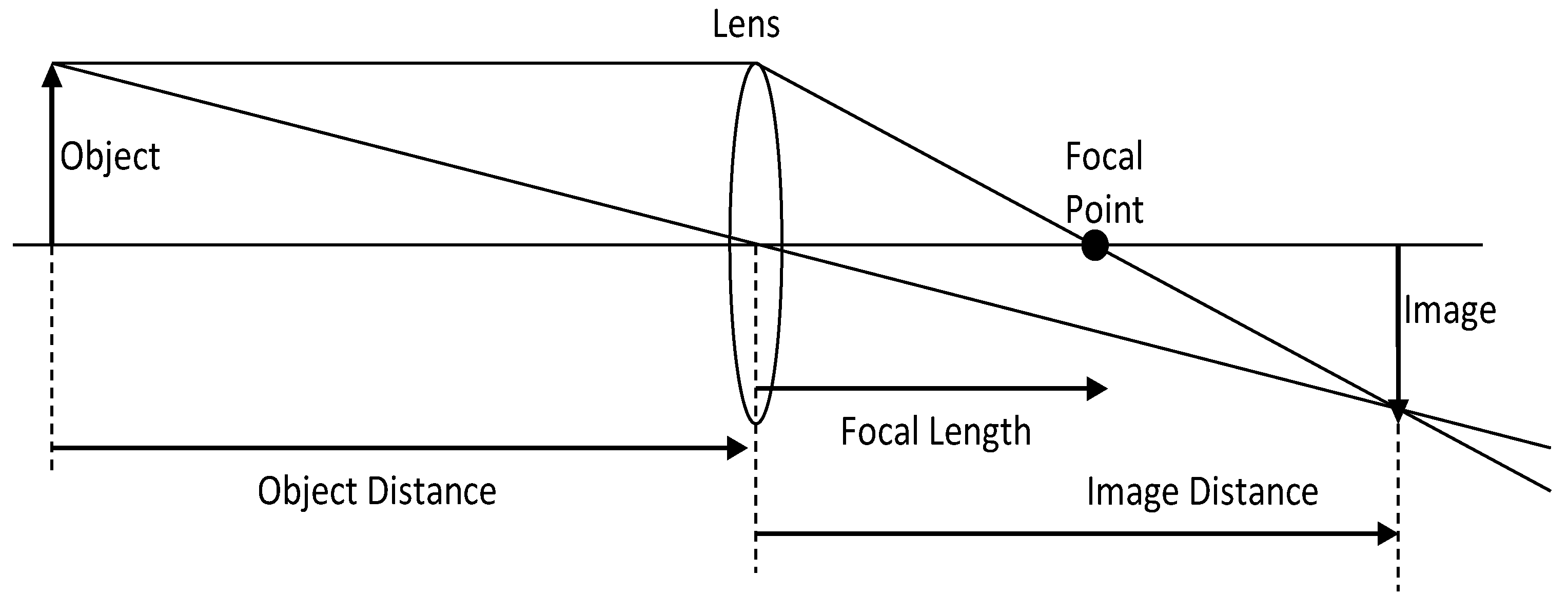
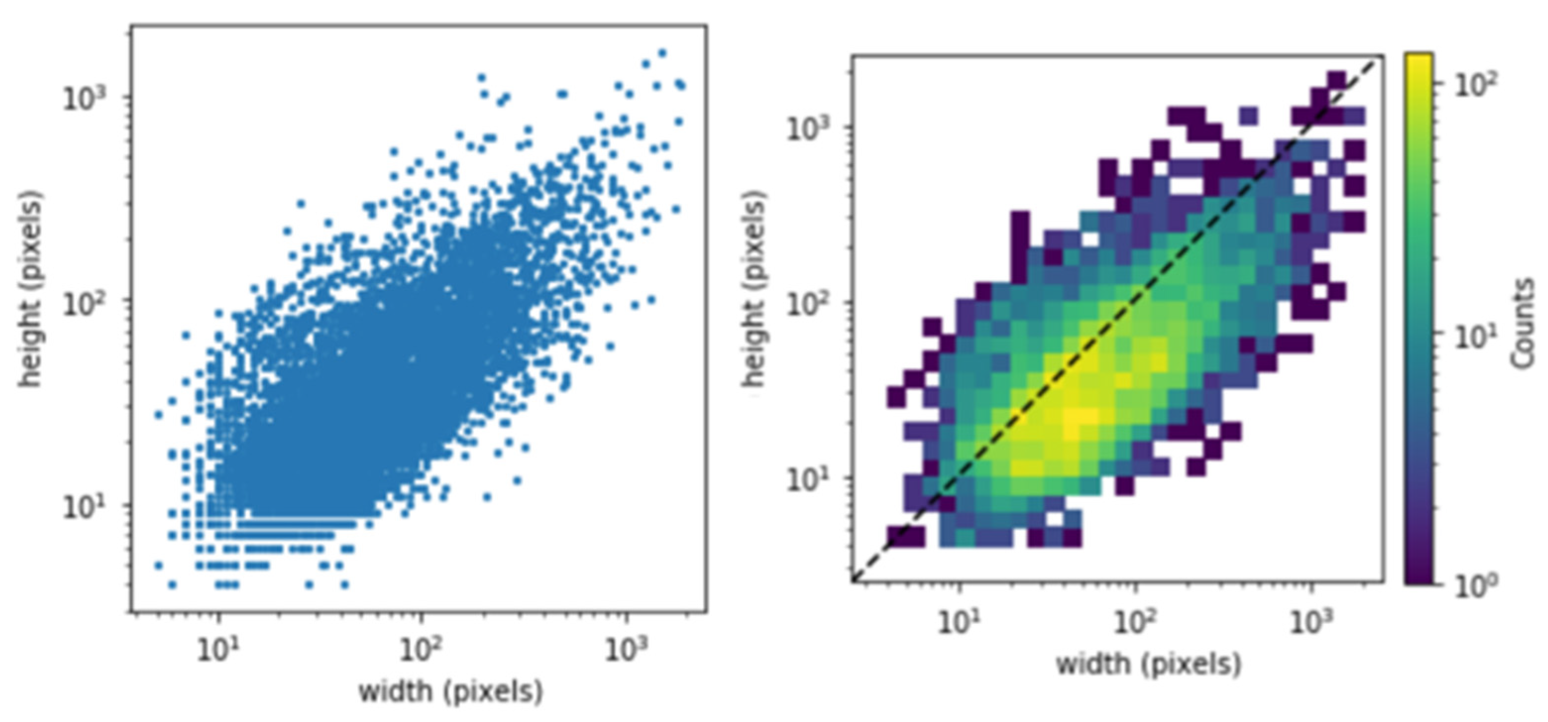
2.1. Data Collection

In the current study, corrosion images were collected from two locations in Melbourne, Victoria, Australia: The Bolte Bridge and sky rail areas. The images of the case projects are presented in Figure 1a,b, respectively. The images were collected from both locations to assess the safety and structural health of case projects. This objective was achieved by including the corrosion dataset for corrosion detection collected at the selected locations. It is preferred to design techniques capable of detecting and localizing infrastructural damages such as corrosion efficiently and cost-effectively [35]. To perform these tasks without interfering with the operational processes, UAVs should be utilized, which are flexible and cost-effective means for capturing images [36]. In the current study, all images were captured using the UAV model DJI-M200 based on vertical take-off and landing (VTOL). Additionally, the quadcopter of DJI-M200 is equipped with three important components: the Global Navigation Satellite System (GNSS) receiver, a barometer, and the Inertial Measurement Unit (IMU) [35].

In the current study, the corrosion detection procedure was started by the collection of an image dataset. The images were extracted from public datasets such as Crack Forest Dataset (CFD), Crack500, and GAPs. The datasets were provided by VERIS, Australia as well. The images were captured using an Unmanned Aerial Vehicle (UAV) with a digital camera. The main data set was raw images that were processed through Seg-Net for label generation and cropped based on desired height and width used as our dataset. For the current study, the target structure was the Bolte Bridge and the SkyRail located in Melbourne, Victoria, Australia (Figure 1a,b). The final dataset contained a total of 1300 images with dimensions set to 4864 × 3648. Each image number of cropped images that was kept was manually supervised based on corrosion level. Each image used was 7 megabytes (MB) and in JPEG format (Figure 2a). The structure degradation detection framework used in the current study is presented in Figure 2b.

Moreover, the images included in the final dataset were divided into four types of corrosion levels: no corrosion, low-level corrosion, medium-level corrosion, and high-level corrosion, as shown in

Table 1. The percentages of pixels in images used for model training and validation.

Item	Corrosion Pixels (%) Classes			Non-Corrosion Pixels (%)	Grand Total (All Corrosion + Non-Corossion Pixels)
	Low	Medium	High
Training	3.61	1.30	0.49	74.60	80
Validation	0.65	0.34	0.26	18.65	20
Total	4.26	1.64	0.75	93.25	100

. A total of 4.26%, 1.64%, 0.75%, and 93.25% pixels were used in the current study for low, medium, high, and no corrosion, respectively, selected by the expert conducting this study. From a total of 6.75% corroded pixels of the final dataset, the used training and validation ratio is 80:20. Training is performed with a total of 5.4% pixels of final dataset, whereas the validation set comprises 1.25% pixels (see Table 1).

The camera installed on the UAV was used to capture the images. The lens collected the light from the object to create an image (Figure 3). The size and location of the image depend on the location of the object and the focal length of the lens. The relationship between the object distance $\left(o\right)$, the focal length $\left(f\right),$ and the image distance$\left(i\right)$ are given by $\frac{1}{o}+\frac{1}{i}=\frac{1}{f}$. The image distance is simply the distance from the object to the thin lines. The image distance is the distance from the thin lens to the image. The focal length is a characteristic of the thin lens, and it specifies the distance at which parallel rays come to a focus. The field calibration at 50 m flight height was carried out with the focal length of 8.4 mm, format size of 7.5 mm, and principal point of 3.8 × 2.5. The drone DJI M200 was used to have a focal length of 24 mm, an operating frequency of 24,000–24,835 GHz, obstacle sensing range 2.3–98.4 feet, a maximum speed of 50.3 mph (S-mode/A-mode) and 38 mph (P-mode), and maximum wind resistance of 12 m/s.

The height and width distributions of the corrosion images included in the final data set are presented as per the four corrosion levels in the current study (Figure 4). An explanation of the spatial location of the corroded area is provided in Figure 4. The overall height and width distributions of corrosion pixels included in the data were obtained using WANDB and Pytorch sessions. Note that the plot only shows corroded pixels distribution. To define positive class images with blob/connected components of more than 3%, corroded pixels are considered after performing a morphological closing operation. Using this procedure, the frequency of corroded pixels was depicted for our data. The data distribution and spatial location are used to locate the labels or bounding boxes of corrosion data. Herein, the axis values define the size distribution of our data set. For our data set, it is notable that the frequency or spatial distribution of the corrosion pixels is not projected closely at one place but rather is well distributed. Moreover, the distribution of the corrosion pixels is not skewed to the left or right side of the plot. Rather, it is centralized, which shows that the data are normal and display a Gaussian distribution. This also indicates that our selected data set of corrosion pixels is not biased.

The final dataset has been divided into four types of corrosion levels. The levels are manually defined based on the segmentation task since all images are randomly cropped in our architecture to 544 × 384 × 3. Further, morphological operation (closing) using a disk of size 3 × 3 has been used to categorize images into sub-classes. The reason for using closing operation is trails that are used as closing fills in the gaps and are smaller than or the same size as the structuring element.

• No corrosion: All images without corrosion (negative class).
• Low-level corrosion: Images having less than 5% of corroded pixels.
• Medium-level corrosion: Images having less than 15% of corroded pixels.
• High-level corrosion: Images having more than 15% of corroded pixels.

Image Pre-Processing and Data Augmentation

After collecting the data set, pre-processing was performed on the captured images for the removal of unwanted objects and noise. This was followed by adjusting the image brightness and size. An important component of the deep networks is the data augmentation procedure. For the current study, the data augmentation was performed 16 times using the following steps:

• The rotation of images to 8 different angles every 45° in [0°, 360°];
• Cropping the rotated image in terms of the largest rectangle without any blank regions;
• Flipping images horizontally at each angle.

2.2. Manual Supervision

The captured dataset has been segmented by the training SegNet model. However, due to its limited accuracy, manual supervision is required. Therefore, we performed per pixel annotation and supervised it manually. While working with general images, the pre-trained model for semantic segmentation is not appropriate for use; therefore, the deep corrosion data set was used to train the SegNet.

The SegNet deep convolutional architecture contains a sequence of encoders, decoders, and a pixel-wise classifier. Generally, the encoder is based on one or more convolutional layers, batch normalization, and rectified linear activation unit (ReLU) non-linearity units, followed by non-overlapping max-pooling and sub-sampling [37]. For the reduction in the overall model parameters and the retention of the class boundaries in segmented images, the decoder displays an unsampled sparse encoding through max-pooling indices. For this study, the end-to-end model training was performed using the stochastic gradient descent method [37], and the general SegNet architecture was modified to Bayesian SegNet. The modification of the architecture was performed using SegNet [37] and SegNet-Basic [38]. Additionally, for the SegNet’s encoder, a VGG-16 network with 13 convolutional layers, was used, followed by 13 corresponding decoders [39].

The CNN is composed of multiple blocks, where the first block is used for feature extraction from an image through the utility of several convolution kernels. This procedure is repeated multiple times, and the last feature map-based values are transformed into a vector that forms the output of the first block and serves as the input for the next block. During the processing in the second block, the input vector values are modified using several linear combinations and activation functions. This results in returning output in the form of a new vector. The end block contains the same number of elements and classes, where each element lies between 0 and 1 and the probabilities are calculated using the logistic or a softmax function activation function. As far as the layers are considered, there are a total of four types of layers in a CNN, namely, (1) convolutional layer, (2) pooling layer, (3) ReLU correction layer, and (4) fully connected layer. The convolution layer is present in the first layer and is responsible for receiving input images and calculating convolution across each filter.

Moreover, the pooling layer is conventionally positioned between two convolution layers and is responsible for receiving feature maps. The pooling layer is responsible for applying pooling operations to these maps, mainly reducing image size by preserving important characteristics. It also plays an important role in reducing the number of parameters and calculations within the network, thus improving the overall efficiency and avoiding the over-learning of the network. Another important component of the CNN is the ReLU correction layer, an activation function responsible for replacing all negative values received as inputs by zeros [40]. Herein, a constant feature size of 64 and a total of four layers were used for each encoder and decoder in the smaller SegNet-Basic network. Therefore, we use the SegNet-Basic as the smaller model for our analysis as it is evident that it provides a conceptually effective representation of the larger architecture. After performing image labeling, all labeled images were re-examined manually using MATLAB for the delicate handling of all corrosion/non-corrosion labels.

2.3. Image Classification and Processing

Generally, the image needs to be resized for the classification network to correspond to the input size, after which high-level features are extracted via the convolutional layers. Then, the fully connected layers utilize the extracted features for the image classification based on the corrosion levels. Ultimately, a particular image will be classified according to four levels of corrosion: no corrosion, low-level corrosion, medium-level corrosion, and high-level corrosion. It is notable that both raw and augmented images were used for the training of our network. The data augmentation based on random image cropping and patching for deep CNNs were used for label generation and corrosion detection in the entire training procedure. Additionally, the input images were resized to 256 × 256 due to the rotation-based transformations. The model training and testing were executed using a single NVIDIA TITAN X graphic card [40].

Considerable advancements have been achieved in classifying and processing images by utilizing the highly expressive deep CNNs displaying numerous parameters [41]. However, the high-performance CNNs are likely to display chances of over-fitting, which might be due to the CNNs memorization of the non-generalized image features present in the training set. Therefore, it is extremely important to use a sufficient set of training samples because utilizing an insufficient set of training samples can cause the model to be over-fitting [42]. However, collecting sufficiently abundant samples is a prodigiously costly attempt that allows for the increased applicability of various data augmentation methods, including flipping, resizing, and random cropping. These augmentation techniques are essentially required to increase the variation in images to prevent model over-fitting [43].

A detailed description of the method adopted in the current study and the proposed CNN architecture is provided in the following subsections.

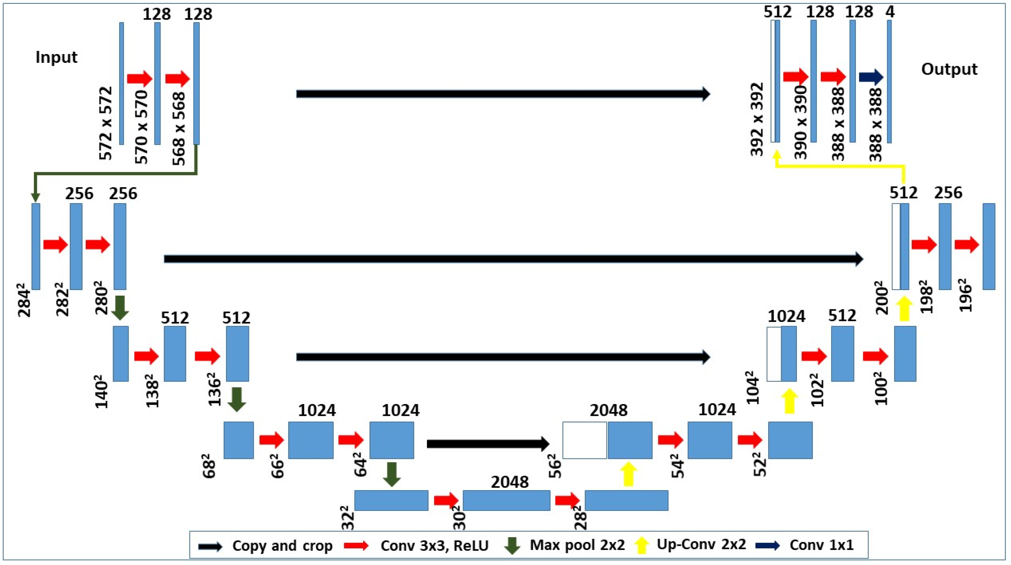
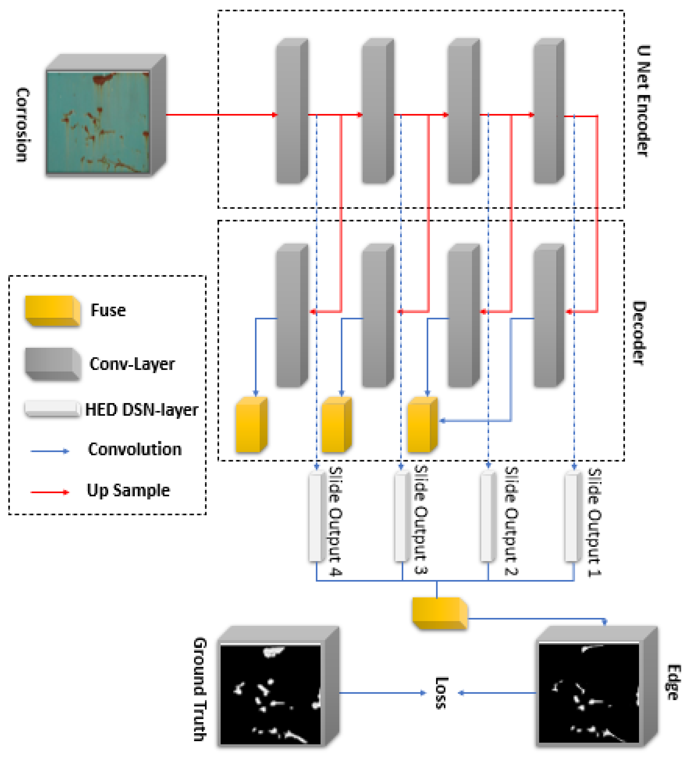
2.3.1. U-Net Model Architecture

A U-Net implementation was used as the model architecture through which important model configurations, including activation, function, and depth, can be passed as arguments during model creation. The U-Net implementation considers the CNNs for precise and quick image segmentation. Such U-Net architectures have emerged as prevalent end-to-end architectures for performing semantic segmentation and can produce very promising results [44]. The overall U-Net architecture of the encoder and decoder used in the study for corrosion detection is presented in Figure 5. The steps followed are given as below:

• A conventional stack of layers and functions is used for the encoder architecture to capture features at different image scales.
• Repeated use of layers $\left(k=3, s=1\right)$ is utilized in each block of the encoder. The non-linearity layer and a max-pooling layer $\left(k=2, s=2\right)$are arranged after each convolution block.
• The decoder architecture is based on the symmetric expanding counterpart of the transposed convolution layers. These layers consider the up-sampling method and a set of trainable parameters to function as the reverse of pooling layers such as the max pool.
• Each convolution block is connected to an up-convolutional layer for the decoder architecture that receives the outputs (appended by the feature maps). This is generated by the corresponding encoder blocks.
• The feature maps for the encoder layer are cropped if the dimensions of any decoder layer are exceeded. Largely, the output is required to pass another convolution layer $\left(k=1, s=1\right)$ that displays an equal number of feature maps and defined labels.

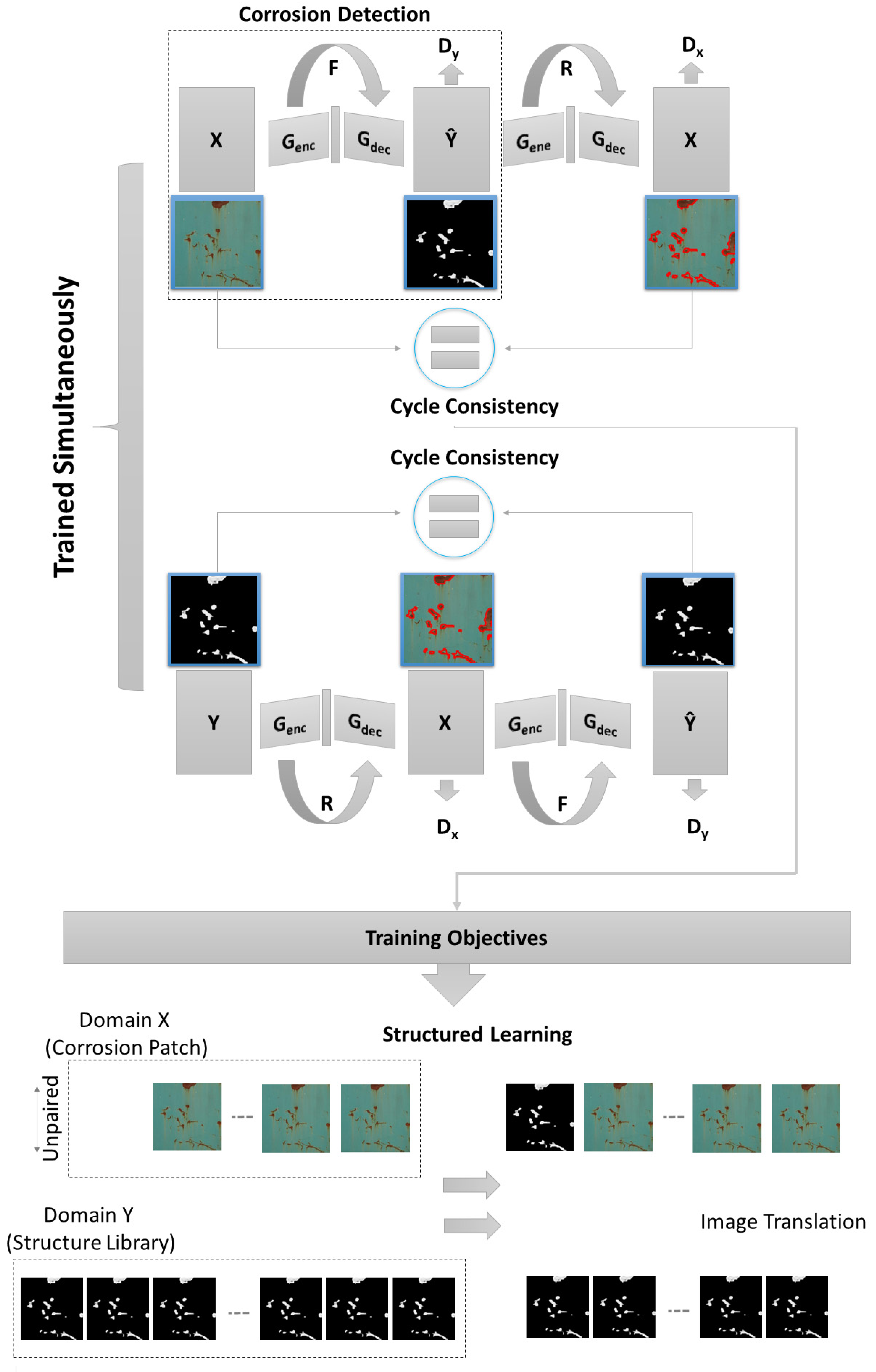
The architectural details described above lead to an elegantly designed u-shaped convolution network that can provide localization and context-based solutions. The accuracy of U-Net architecture is 6.1% higher than FCN (Fully Convolutional Network) architecture for the 256 × 256 dataset. For dataset 512 × 512, although the validation accuracy of U-Net architecture is 1% less than FCN, for memory footprint, U-Net is better than other variants. In comparison with U-Net, Seg-Net has a similar design. The main difference is the depth (channels), whereas the overall accuracy is almost similar. Therefore, the usage of Seg-Net or U-Net is often considered a developer choice.

Each blue box in Figure 5 represents a multi-channel feature map with the number of channels mentioned on top of the box, and the $x-y-size$ is provided at the lower-left edge of the box, whereas the white box corresponds to the copied feature maps, and the arrows indicate different operations.

We employed a multi-scale feature Decode and Fuse (MSDF) model with a Conditional random fields (CRF) layer for the current study for boundary detection (Figure 6). Furthermore, we also used this model to implement the probabilistic inference over the segmentation model. Therefore, for the given training data $X$ with labels $Y$ and probability distribution $p$, we use the Bayesian SegNet to explain the posterior distribution over the convolutional weights $\left(W\right),$ as denoted by the following expression:

$$p(W|X,Y)$$

(1)

Since the posterior distribution is not manageable, an approximation of the weight distribution is essential for which we utilize the variational inference that allows distribution learning over the network weights $q(W$) This is achieved through the Kullback–Leibler $\left(KL\right)$ divergence minimization amid the approximated distribution and the full posterior, described as follows:

$$KL(q\left(W\right)\parallel p(W|X,Y))$$

(2)

For each $K\times K$ dimensional convolutional layer $\left(i\right)$ with units $j$, vectors of Bernoulli distributed random variables bi and variational parameters $Mi$ (in the approximated variational distribution $q \left(Wi\right)$) allow one to achieve an approximated model of the Gaussian process and the approximated model of the Gaussian process can be described mathematically, as shown in Equation (4).

$$bi,j\sim Bernoulli\left(pi\right)forj=1,\dots ,Ki$$

(3)

$$Wi=Midiag\left(bi\right)$$

(4)

For this study, we used a standard value of 50% to account for the probability $\left(pi=0.5\right)$ of dropping for probability optimization of neurons to avoid overfitting while training. For the network training, the utilization of the stochastic gradient descent allows for effective learning of the weight distribution that assists in obtaining a better explanation of data and avoiding model over-fitting. For model training, we use the dropout method, which aids in achieving a posterior distribution of SoftMax class probabilities. For segmentation prediction, the means of these samples are employed. In comparison, the output uncertainty associated with each class is modeled by the variance estimation, estimated by taking the mean of the variance measurements per class.

2.3.2. CycleGAN

The CycleGANs offer effective network training without requiring manually labeled Ground Truths. This is mainly because CycleGANs allow for the translation of corrosion images to the Ground Truth, such as images with similar structural patterns [45]. The proposed approach will help government/municipalities by providing a scalable, real-time, robust, and efficient technique to conduct a cost-effective inspection to maintain or detect structural damages. We propose a conceptual framework for an automated corrosion detection system using modern machine learning techniques (deep neural network). This can be easily scaled to any edge device, e.g., jetson nano or coral dev board. Two separate data sets are required for training a CycleGAN. These include the corrosion images $\left\{xi\right\}$ in the corrosion image set $\left(X\right)$, and the images $\left\{yi\right\}$ in the structure library $\left(Y\right)$, respectively. The network topology is based on the forward and reverses GANs that perform image translations from $X$ to $Y$ $\left(F: X \to Y\right)$ and $Y$ to $X \left(F: Y \to X\right)$. The overall topology is presented in Figure 7. The CycleGAN is used to transfer or distribute the characteristics of an image to another image.

The CycleGAN addresses problems through image reconstruction. Generally, the CycleGAN has two core components: the generator and discriminator. The generator produces the samples from the desired distribution, whereas the discriminator helps determine whether the sample is from a real distribution or a generated one. The CycleGAN comprises three parts: (1) encoder, (2) transformer, and (3) decoder. The steps for CycleGAN are given as below:

• At first, the input image (x) is taken and converted to a reconstructed image based on the generator (G).
• Next, the process is reversed to convert a restructured image to an original image through the generator (F)
• Later, the mean squared error loss between real and reconstructed images is calculated.

The input images are received by the encoder, which extracts input features using convolutions. The encoder is based on three convolutions that help reduce the image to 1/4th of its actual size. After applying the activation function, the output of the encoder is transferred to the transformer based on 6 or 9 residual blocks depending on the input size. Similarly, the transformer’s output is transferred to the decoder, which utilizes a 2-deconvolution block of fraction strides that helps increase representation size compared to the original size [34].

Generally, for the CycleGAN working, there are two discriminators for the system, mainly $Dx$ and $Dy$. The discriminator $Dx$ is used for distinguishing between the $\left\{xi\right\}$ and $\left\{R\left(yi\right)\right\}$ with $L_{advr}$ (reverse adversarial loss). Further, the discriminator $Dy$ distinguishes between $\left\{yi\right\}$ and the translated images $\left\{F\left(xi\right)\right\}$ to overcome the differences in consistency to domains and data imbalance. Finally, the objective function can be described using Equation (5), where $L_{advf}$ indicates the forward adversarial loss.

$$L=\left(L_{advf}+L_{advr}\right)+\lambda \left(L{1}_{fc}+L{1}_{rc}\right)$$

(5)

In the objective function, $\lambda$ controls the weight between the two losses (adversarial and the cycle-consistent loss), and $L{1}_{fc}$and $L{1}_{rc}$ represent the two-cycle consistent losses with $L1$-distance formulas in the forward and reverse GAN, respectively [45].

2.4. Loss Formulation

The loss formulation is based on adversarial loss and cycle-consistency loss. The adversarial loss provides the benefit of obtaining structured images. However, when used solely, it is insufficient to translate the corrosion image patch to the desired structure patch or vice versa. Owing to this, the consistency of structure pattern amid the input and the output images is not guaranteed. Thus, an extra parameter for cycle consistency is necessitated for the effective network training and maintenance of the structure pattern consistency between the input and output [34].

2.4.1. Adversarial Loss

The adversarial networks execute through the max–min two-player game. The training based on these networks can assist in achieving real-like images that are generated from noise. Therefore, the alternate optimization of the following objectives of the adversarial networks is very important.

$$ma{x}_D{V}_D\left(D,G\right)=E_{XP{4}^{\left(X\right)}}\left[logD\left(x\right)\right]+E_{zP{4}^{\left(z\right)}}$$

(6)

$$ma{x}_G{V}_G\left(D,G\right)=E_{zP{4}^{\left(z\right)}}$$

(7)

In Equations (6) and (7), D refers to discriminator, G refers to the generator, z refers to noise vector input into the generator, and $x$ refers to the real image in the training set. $G$ generates images $\left(Gz\right)$ that are like images from $X. D$ distinguishes between the real samples ‘$x$’ and the generated sample $G\left(z\right)$. Equations (6) and (7) are being maximized by $D$ and $G$, leading to adversarial learning.

2.4.2. Cycle-Consistency Loss

For the data set $X$, each sample ‘$x$’ should be able to return to the original patch through the network after the processing cycle $(x$ → $G\left(x\right) \to F\left(G\left(x\right)\right) ~ x)$. Similarly, for each structure image ‘$y$’ in the structure set, the network should allow for the return of y back to the original image $(y \to R\left(y\right) \to F\left(R\left(y\right)\right) ~ y$). $E_{xp{4}^{\left(x\right)}}$ defines the expected probability distribution. These constraints lead to the formulation of cycle-consistency loss, which can be defined using Equation (8).

$$L_{cyc}\left(F,R\right)=E_{xp{4}^{\left(x\right)}}$$

(8)

A general mathematical expression can be used for the image edge detection problem, where an image in the data layer can be transformed into a multidimensional matrix and the set of edge feature pixels of the Ground Truth can be denoted by the variables $Xn$ and $Yn,$ respectively, as shown in Equation (9).

$$Yn=\left\{yj\left(n\right),j=1,\dots ,\left|Xn\right|\right\}$$

(9)

In Equation (9), $\left|Xn\right|$ denotes the number of pixels in the image $n$. The possibility of predicted pixel labeled by the annotator is represented as follows:

$$P(yj=1|Xn)$$

(10)

The values are obtained as zero and one, where zero means that the edge pixel predicted by the model is not the Ground Truth label, and one shows that the edge pixel predicted by the model is labeled by all annotators.

Each pixel is annotated, and a value of 0.7 was set as the threshold $\left(\mu \right)$ based on training data in the loss function. A pixel should not be used if the value of $P(yj=1|Xn)$ is greater than 0 and less than $\mu$ because the pixel is considered controversial. The training data of images can be described using Equation (11).

$$S=\left\{\left(Xn,Yn\right),n=1,2,\dots ,N\right\}$$

(11)

where $N$ is the number of images used for training. For every pixel, the loss functions are computed for both the top-down architecture and the decoder subnet regarding the Ground Truth pixel label, using Equations (12) and (13).

$$IfP(yj=1|Xn)>\mu$$

(12)

$$l_{side}\left(W,X_n\right)=-\beta {\displaystyle \sum }_{jϵy^{+}}logP\left(y_j=1|X_n,W\right)-\left(1-\beta \right){\displaystyle \sum }_{jϵy^{-}}logP\left(y_j=0|X_n,W\right)$$

(13)

If $P (yj=1|Xn)<\mu$ then lside $\left(W, Xn\right)=0$. For this particular instance, Equation (14) is used.

$$\beta =\frac{\left|Y-\right|}{\left|Y-\right|+\left|Y+\right|},1-\beta =\frac{\left|Y-\right|}{\left|Y-\right|+\left|Y+\right|}$$

(14)

where $Y+represents$ the edge label and $Y-refers$ to the non-edge label.

It is extremely important to consider the fusion loss while calculating the total loss function for a multi-scale model. This method for calculating fusion loss assumes that the top-down architecture has the same loss function as the decoder subnet. Further, the value $W$ is learned and subsequently updated during the training procedure. The improved loss function version is represented using Equation (15).

$$l\left(W,X_n\right)={\displaystyle \sum }_{i=1}^N({\displaystyle \sum }_{j=1}^M{l}_{side}^j\left(W,X_n\right)+l_{fuse}\left(W,X_n\right))$$

(15)

where $N$ represents the number of images used for training and $M$ denotes the total number of Holistically-Nested Edge Detection (HED) dsn-layers and the layers of decoder subnet (set to 6 for this study). Similarly, $l_{fuse}\left(W,X_n\right)$ represents the loss function associated with the fusion layer.

2.4.3. Model Parameters

The network was built based on top of implementations (i.e., Fully Convolutional Network (FCN) , Deeply Supervised Network (DSN), Holistically-Nested Edge Detection (HED), and SegNet. It was trained using the Caffe library. The Stochastic Gradient Descent (SGD) based optimization was used for the model. The parameters considered for this study and the associated tuned values are represented in

Table 2. Model parameters tuned for the network.

	Parameter	Value Tuned
(1)	Size of the input image size	544 × 384 × 3
(2)	Ground truth size	544 × 384 × 1
(3)	Size of mini-batch	1
(4)	Learning rate	1 × 10−4
(5)	Loss weight associated with each side-output layer	1.0
(6)	The loss weight associated with the final fused layer	1.0
(7)	Momentum	0.9
(8)	Weight decay	2 × 10−4
(9)	Training iterations	2 × 105; reduce learning rate by 1/5 after 5 × 104

.

In the current study, we utilized batch normalization, side-output layers, and loss-of-function elaboration for our network principally to distinguish the four levels of corrosion. For our model, the learning rate; loss weight of each side-output; loss weight of each momentum; and decay values of 1 × 10⁻⁴, 1.0, 1.0, 0.9, and 2 × 10⁻⁴ were used, respectively (Table 2). The size of the images was scaled according to the size of the input images. The in-depth analysis of local images was performed using image segmentation.

Moreover, variable mini-batch sizes can be used depending on the GPU capacity. For the current study, a mini-batch of 1 was used to reduce the time required for training. The learning rate starts from 0.0001 but is later adjusted based on momentum and weight decay. This is performed for the training optimization and avoiding getting stuck at the local minima. The utilization of the described architecture assists in improving the convergence and accuracy subsequently. It also eliminates the requirement of using pre-trained models for network training.

3. Model Development and Training

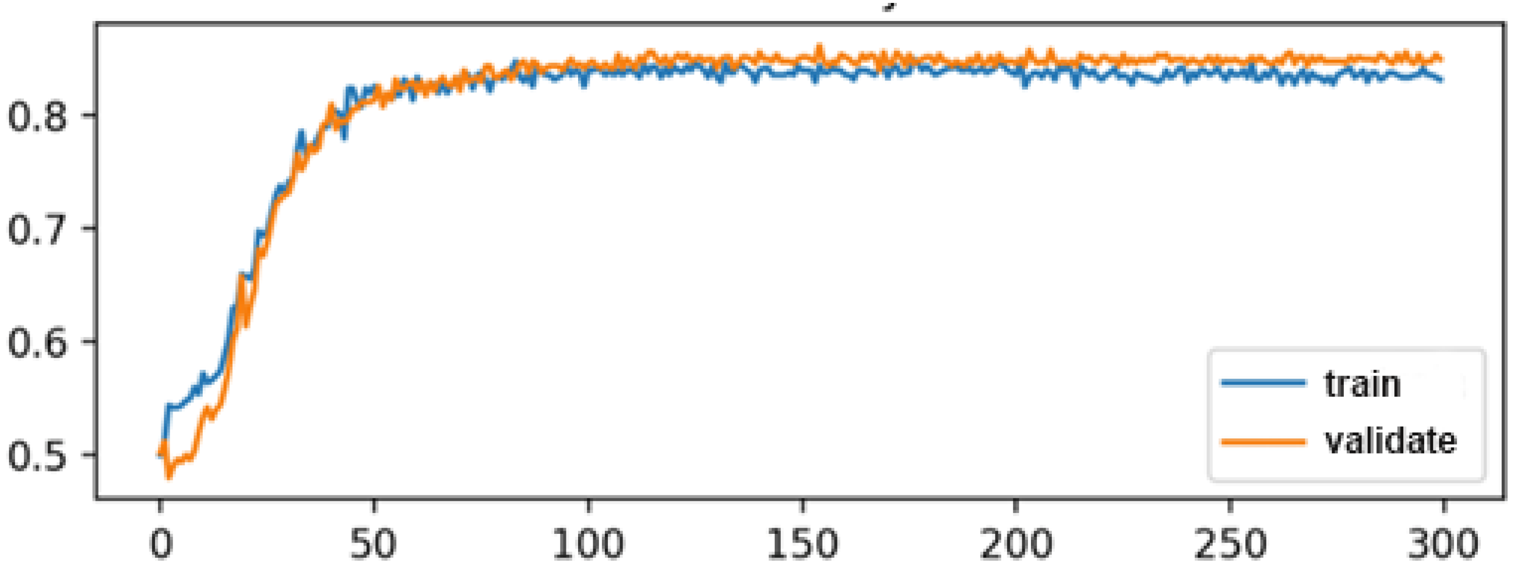
This section explains the development and implementation of the model developed in this study.

3.1. Model Training

Various tools, functions, and criteria such as a loss function, optimizer (Stochastic Gradient Descent (SGD)), device (CPU/GPU), learning rate scheduler, epoch (number from where to initiate training), training, and validation data loader were used to train the U-Net architecture. Training U-Net is based on iterating over the training data loads and sending the batches to the training mode through the network. Training of the U-Net architecture produces outputs/results in the three forms: accumulated training loss, validation loss, and learning rate. Thus, an extra parameter for cycle consistency is necessitated for the effective network training and maintenance of the structure pattern consistency between the input and output. The training rate range test results on our data set (for both the training and validation loss) were analyzed using the matplotlib. The data used in the current study do not display overfitting or bias. Since we are using both the training and test sets, we adopt a better and generalized strategy that can also be applied to unseen data to give better performance and accuracy. It is also shown that for both the training and test set, a comparable performance was achieved after 50 iterations (Figure 8).

3.2. Evaluation Metrics

For the evaluation of common semantic segmentation, three metrics were used in the study. We calculated the Global Accuracy (GC), Class Average Accuracy (CAC), and the mean Intersection of the Union (IoU) over all classes. Additionally, three other metrics, including precision (P, Equation (13)), recall (R, Equation (14)), and F-score (F, Equation (15)), were used for the evaluation. Finally, the GC estimates the percentage of correctly predicted pixels and is calculated using Equation (16). Here, n and t refer to the sample and technique currently under observation.

$$\mathrm{GC}={\displaystyle \sum }_i{n}_{ii}{\displaystyle \sum }_i{t}_i$$

(16)

The CAC estimates the predictive accuracy over all the classes and is presented by Equation (17).

$$\mathrm{CAC}=\left(\frac{1}{n_{cls}}\right){\displaystyle \sum }_i{n}_{ii}/t_i$$

(17)

The mean IoU over all classes was calculated using Equation (18), where n is the sample and t is the technique currently under observation.

$$\mathrm{IoU}=\left(\frac{1}{n_{cls}}\right){\displaystyle \sum }_i{n}_{ii}/t_i+{\displaystyle \sum }_j{n}_{ji}-n_{ii}$$

(18)

Further, P, R, and F were also calculated to evaluate the semantic segmentation using Equations (19)–(21).

$$\mathrm{P}=\frac{no of true positives}{ no of true positives+no of false positives}$$

(19)

$$\mathrm{R}=\frac{no of true positives}{ no of true positives+no of false negatives}$$

(20)

$$\mathrm{F}=\frac{2\mathrm{PR}}{\mathrm{R}+\mathrm{R}}$$

(21)

Since the P and R metrics do not consider the true negative rates, the concept of the Receiver Operating Characteristic (ROC) curve was employed for the evaluation. The True Positive Rate (TPR), False Positive Rate (FPR), and the Area Under the ROC Curve (AUC) are calculated using Equations (22) and (23), respectively.

$$\mathrm{TPR}=\frac{no of true positives}{ no of true positives+no of false negatives}$$

(22)

$$\mathrm{TPF}=\frac{no of false positives}{ no of false positives+no of true negatives}$$

(23)

3.3. Training and Test Accuracy

To assess the accuracy of the training and test set, mean average precision $\left(\mathrm{mAP}\right)$ and $\mathrm{IoU}$ parameters were used in the current study. The P values were plotted on the x-axis and the $\mathrm{R}$ values on the y-axis, respectively. Precision (P) is defined as the positive predictions for a positive class, whereas the $\mathrm{R}$ metric quantifies positive predictions for all positive classes included in the dataset. These parameters were used for the evaluation of image segmentation. Here, the IoU metric is used to quantify the percent overlap between a target mask and the predictions of the output results. In other words, the IoU parameter can measure or quantify the number of overlapping or common pixels between a target mask and the predictions of the output results. For the selected data, the value of the $\mathrm{IoU}\_\min$ was increased from 0.1 to 0.9 while calculating the error on each point, as shown in Figure 9.

It was observed that when the value $\mathrm{IoU}\_\min$ was equal to 0.1, the value of $\mathrm{mAP}$ was maximum (0.77). This indicates that the threshold should be high. However, while increasing the $\mathrm{IoU}\_\min$ from 0.1 to 0.9, an observable decrease in the values of $\mathrm{mAP}$ is observed for our data set (Figure 9). The threshold must not fluctuate; otherwise, the average accuracy will be compromised. The P should be high for a model, and R-value should be lower. In the current study, we have computed the P-R curves by changing the prediction confidence threshold. The process was repeated for different $\mathrm{IoU}$ thresholds to establish a match. Further, in our model, the computation of a single$\mathrm{P}$ and R score at the specified $\mathrm{IoU}$ threshold did not adequately describe the behavior of our model’s full P-R curve. Therefore, we utilized the average $\mathrm{P}$ to integrate the area under a P-R curve effectively.

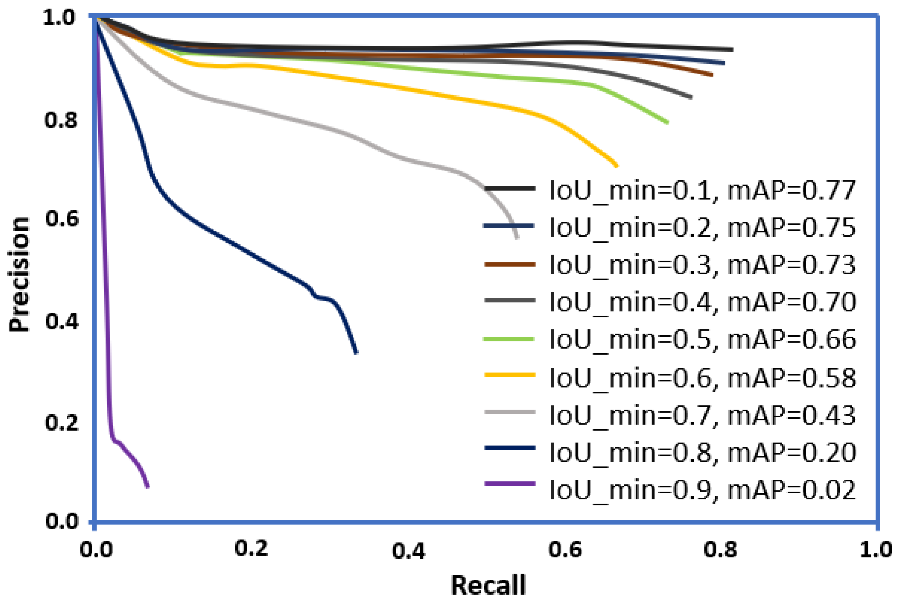
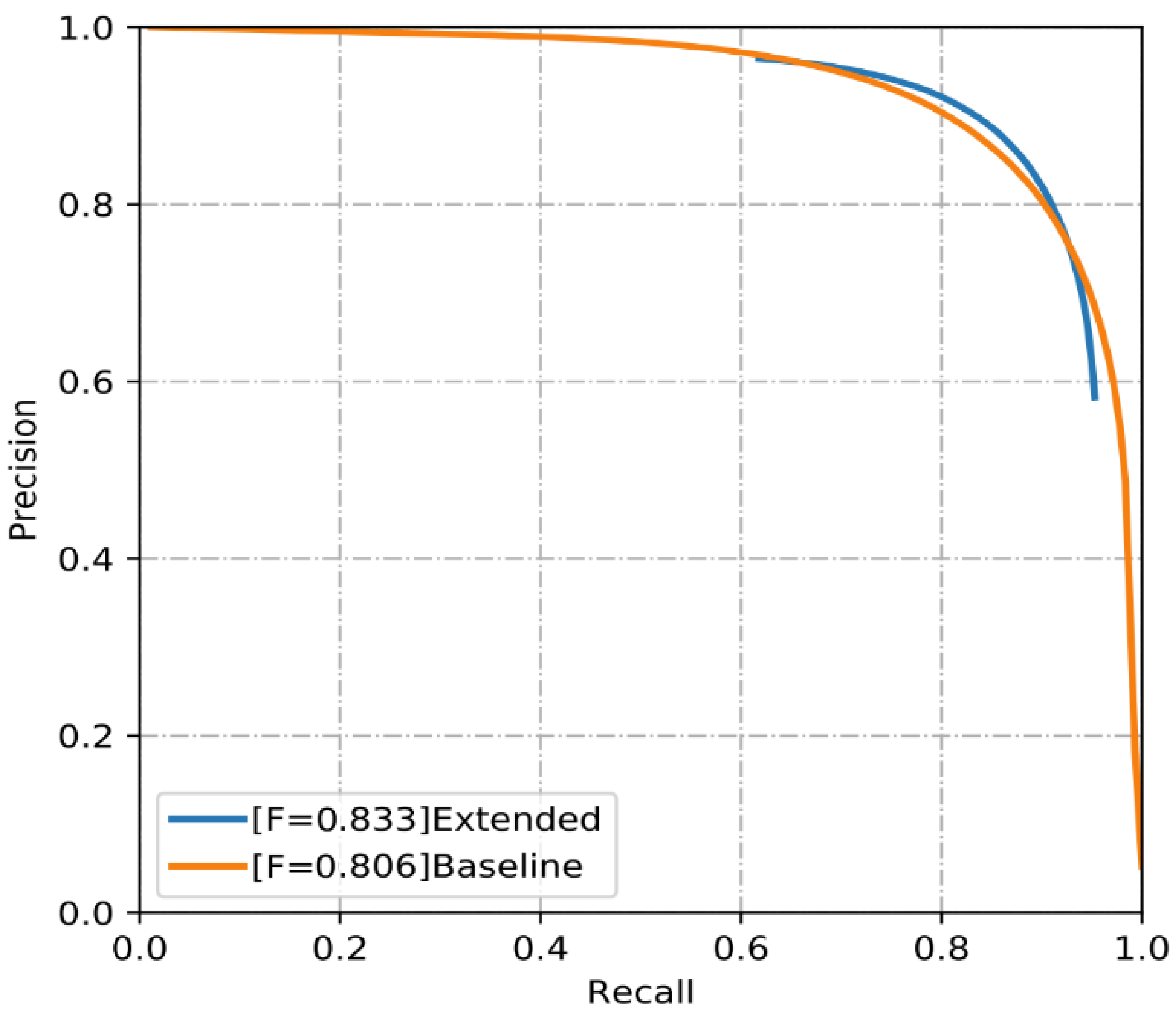
3.4. Evaluation of Network Performance

The network for corrosion detection was trained using six approaches, namely, (1) DeepCorrosion-Basic, (2) DeepCorrosion-BN, (3) DeepCorrosion-CRF, (4) DeepCorrosion-GF, (5) DeepCorrosion-CRF-GF, and (6) DeepCorrosion-Aug. The HED and loss-of-function architecture were used in the DeepCorrosion-Basic. This approach was used for the training of a set of 3000 original images. The DeepCorrosion-BN is the modified version of DeepCorrosion-Basic, where, before every activation operation, the batch normalization layers are added. The architectures of DeepCorrosion-BN and DeepCorrosion-CRF are similar, but they differ concerning the variations in the addition of the CRF after the network. The same holds for the DeepCorrosion-GF, which is a DeepCorrosion-BN based version with an addition of the guided filtering module. The DeepCorrosion-CRF-GF approach is based on the linear combination of the two approaches, namely, DeepCorrosion-CRF and DeepCorrosion-GF, and is described using Equation (24).

P = βP CRF + (1 − β) PGF

(24)

where $\mathrm{P}$ is the prediction map, and β is the balancing weight with a value of 0.5. The precision-recall curves generated by the threshold segmentation method used in the current study is shown in Figure 10 below.

We have used the PSPnet based multi-focus method for image fusion. Moreover, the DEEPLAB method was used for the semantic image segmentation using deep CNNs, Atrous Convolution, and Fully Connected CRFs. Herein, the Pyramid Scene Parsing Network (PSPnet) is used to extract the focused region of an image. In comparison, DEEPLAB was utilized for the optimization of the segmentation map to achieve map refinement. We have used baseline and extended architecture for the current study. We have added data augmentation, fusion method, and decay of learning rates in the extended architecture method. However, in the baseline method, data augmentation has not been applied. The results of both the baseline and extended methods are presented in Figure 10.

The P-R curves obtained for both the methods indicate that the extended method displays better performance, as indicated by the F-Score value of 0.833 compared to the baseline method (F-Score of 0.806), as shown in Figure 10.

4. Results and Discussions

Early detection and concurrent maintenance form an integral part of the structural health monitoring system used for civil infrastructures. If left unprotected, the damage caused to infrastructures can lead to serious losses in terms of economy and loss of human lives [4]. Therefore, designing cutting-edge technologies to monitor the health of infrastructures such as bridges is of extreme importance to ensure the health of civil infrastructures and the safety of human lives and to reduce financial losses [17]. However, the traditional manual or human-based visual inspection methods that were conventionally used to monitor the structural health of civil infrastructures display different limitations [46]. To overcome the limitations associated with traditional inspection methods, it is necessary to use advanced computer vision-based and artificial intelligence (AI) techniques, such as artificial neural networks (ANNs) and convolutional neural networks (CNNs), to assess the health of civil infrastructures.

Therefore, in the current study, we proposed a modified version of deep hierarchical CNN architecture, based on 16 convolution layers and cycle generative adversarial network (CycleGAN), to predict pixel-wise segmentation in an end-to-end manner. This was achieved through image collection (1300 images) from two target locations, mainly the Bolte Bridge and sky rail areas in Victoria (Melbourne), using the DJI-MJ200. The images were collected to train our deep learning model. To detect corrosion on civil infrastructures such as bridges, an in-depth analysis of local images was conducted using image segmentation that was performed through the representation of the subject into the binary images. Herein, the total image set was divided into the training set and the test set, respectively. We have presented some of the representative images collected from the target locations, and the corresponding segmentation used in the current study is also presented in Figure 11.

The segmentation was performed through the representation of subjects in the binary images. The pixel-wise segmentation map was used for each image that allowed the exact coverage of the corrosion regions. The images were set to a pixel size of 544 × 384. The corrosion images were chosen from a wide range of scales and scenes to achieve the universal representation of corrosion. Furthermore, the images included in the dataset were divided into four types of corrosion levels: no corrosion (93.25%), low-level corrosion (4.23%), medium-level corrosion (1.32%,) and Hhigh-level corrosion (1.20%), as previously presented in Table 1. Thus, about 95.16% non-corrosion pixels and 4.84% corrosion pixels were included in the training set.

In comparison, 94.01% non-corrosion pixels and 5.99% corrosion pixels were included in the test set (Table 1). The statistics for the annotation of the major textures and scenes distribution are shown in Figure 11. Figure 11a,b represents the input and output water straining images of the case study projects, whereas Figure 11d,f,h represent the water straining input images used to obtain the output images Figure 11e,g,i respectively. The input and output images for corrosion are presented in Figure 11j–m, where the left panel corresponds to input and the right panel corresponds to the output images. The corrosion images were chosen to achieve the universal representation of corrosion, as shown in the data distribution previously in Figure 4. Figure 11a–m depicts water straining, and Figure 11c shows the suppression of the background image to extract water straining. Figure 11n represents water straining, and Figure 11o depicts corrosion severity. There are different shades of grey, but from a practical standpoint, a grey spectrum can be divided into a limited number of levels, i.e., grey level Figure 11p–z1.

The colored image is converted to grayscale with predetermined grey levels to build the matrix. For example, Figure 11p shows a grey-scale patch, and Figure 11r represents its corresponding grey levels. Figure 11r,u,x,z1 represents the detected corrosion. Despite other structures in the images, the prediction gives a high score for the area where positive classes are present. For the proposed CNN framework, the total corrosion pixels included in the training and test sets were further distributed into significant and weak corrosion pixels, respectively (Figure 11). This classification was performed to distinguish corrosion pixels based on the pixel width. For example, corrosion with a pixel depth of 0 to 5 was categorized with corrosion and water straining.

Similarly, corrosion with a pixel width above 5 depicts object features. Moreover, a data augmentation approach based on random image cropping and patching was used for the proposed deep CNN architecture for label generation and corrosion detection during training. The frequency of corrosion pixels was predicted, and related labels or bounding boxes were located using data distribution and spatial location.

A batch normalization, side-output layers, and loss-of-function elaboration were used for our network, principally to distinguish four levels of corrosion in the current study. A reduced over-fitting of the network and a significant boost in the performance can be achieved using batch normalization. In addition, both conditional random fields and the faster/efficient guided image filtering methods can be implemented to refine the dense regions. In the current study model, parameters such as learning rate, loss weight of each side-output, loss weight of each final fused layer, momentum, and decay were considered, as shown in Table 2. A mini-batch size of 1 was used to reduce the time required for training.

We have proposed two models in our study that are the baseline and extended architectures (Figure 10). In the baseline method, data augmentation has not been applied, whereas in the extended architecture method, we have added data augmentation, fusion method, and decay of learning rates. Overall, we assessed the performance of two proposed methods (i.e., baseline and extended). The performance was also evaluated for three different methods, including the PSPNet, DeepLab, and SegNet. It was evident that the extended method displayed superior performance compared to all other models, as shown by the performance evaluation metrics presented in

Table 3. The statistics for the used threshold segmentation methods.

Outputs	Global Accuracy	Class Average Accuracy	Mean IoU	Precision	Recall	F-Score
Extended	0.989	0.931	0.878	0.849	0.818	0.833
Baseline	0.983	0.899	0.892	0.83	0.784	0.806
PSPNet	0.962	0.873	0.822	0.785	0.724	0.753
DeepLab	0.932	0.82	0.76	0.725	0.654	0.687
SegNet	0.870	0.815	0.642	0.625	0.66	0.642

. The performance of models was assessed using parameters such as GC, CAC, Mean IOU, P, R, and F-score.

In addition, cross-validation was performed on each architecture, and the prediction for each method was assessed using the described evaluation metrics. The statistical parameters for all five models, including proposed methods (extended and baseline), PSPNet, DeepLab, and SegNet, are presented in Table 3. The SegNet method is sensitive to noise and incorrectly extracts data with more shadows and stains. Lack of contextual information to acquire different types of cracks may lead to changes in the width of the cracks. While PSPNet effectively eliminates the influence of noise, it loses more detailed information. DeepLab performs better in extracting light cracks and can eliminate most of the noise interference, but non-existent cracks are produced at large dilation rates, and its single convolution kernel size may cause a loss of crack information.

Similar to our study, various authors have also described the importance of CNN-based deep learning methods for damage detection of civil infrastructures with variable performance statistics. Moreover, the utility of CNNs for corrosion detection has been extensively reported in the literature. Cha et al. [18] have adopted Faster R-CNN for the detection of multiple damages on civil infrastructures. The authors used a total of 2366 images with 500 × 375 pixels, and the evaluation of their model revealed average precision values of about 90.6%, 83.4%, 82.1%, 98.1%, and 84.7% for concrete crack, steel corrosion (medium or high), bolt corrosion, and steel delamination damage types, respectively. Particularly for this study, the CNN-based method showed better accuracy.

Moreover, Atha and Jahanshahi reported using CNN-based networks, namely, ZF Net and VGG16, compared with three other proposed CNNs (i.e., Corrosion7, Corrosion5, and VGG15) for the detection of corrosion [4]. Overall, for these models, the F-Scores were observed between 91.96 to 98.64%, and the P and R values were found to be 90–98.31% and 65.64–98.64%, respectively [4]. The fine-tuned VGG-16 network outperformed all other methods showing F-Score, R, and P values of 98.47%, 98.31%, and 98.64%, respectively [4]. Additionally, Forkan and coworkers have reported the development of a CorrDetector framework for corrosion detection and feature extraction. The CorrDetector was based on the novel ensemble of deep learning CNNs. Seven different methods were evaluated in the study, including a simple CNN, $\lambda C$ model, Corrosion 5, Corrosion 7, Inception V3, Mobilnet, Resnet50, and VGG16 [29]. Overall, their proposed λC model displayed the best performance for segment-level and image-level predictions compared to all other methods. Accuracy (92.50%), precision (96.01%), recall (95.91%), and F-score (98%) of $\lambda C$ model were the highest for the image-level predictions [29].

However, if we consider the performance of our proposed models (i.e., extended, baseline, PSPNet, DeepLab, and SegNet) in the current study, it is evident that the extended method outperformed all other methods, thus showing GC, CAC, mean IOU, P, R, and F-score values of 0.98, 0.93, 0.87, 0.84, 0.81, and 0.83, respectively, as shown in Table 3. Notably, our extended and baseline models display higher accuracies of about 0.989% and 0.983%, respectively. As far as the overall performance evaluation parameters are considered, it is evident that our proposed models display performance measures within a comparable range of the previously reported studies [4,29]. Moreover, the lowest performance was obtained in our study using the SegNet architecture as indicated by the evaluation parameter values. The PSPNet and DeepLab architectures displayed better performance in comparison to the SegNet method. Most prominently, the baseline method also outperformed the PSPNet, DeepLab, and SegNet architectures. If we compare the proposed baseline and extended methods, it is evident that the performance of the extended method was slightly better than the baseline method. Notably, the baseline did not perform good generalization because we added a weighted average instead of simple fusion averaging. However, in the extended architecture, we performed CRF-based fusion. Therefore, it is evident that the proposed network architecture in the current study displays a considerable improvement in the overall performance compared to the methods included in this study (i.e., PSPNet DeepLaband and SegNet) and methods used in other studies reported in the literature. Moreover, variations are observable in the results of the methods, mainly due to the presence of certain intrinsic differences between the corrosion detection and edge detection methods. Therefore, we can conclude that the extended model is ideal for real-time image processing of corrosion images, while the lowest performance was obtained for corrosion assessment using the SegNet.

Generally, the major challenge in damage identification is the characterization of the unknown relationships between measurements and patterns of damages for the subsequent selection of damage indicators. This requires the utilization of dense sensor array and complex algorithms for data processing, producing computational complexity. The proposed CNN-based architecture proposed in the current study is highly efficient at detecting corrosion features with greater accuracy due to pixel-wise segmentation. It also helps in overcoming processing overhead and computational intensity. Additionally, the utility of CNN-based architecture allows for the exploration and learning of abstract features and complex classifier boundaries that allow distinguishing various attributes of the problem under study. Moreover, the proposed CNN-based architecture is less prone to noise in images and thus allows for the efficient detection and localization of corrosion. Using CycleGAN and U-Net together in the CNN-based architecture provides the advantage of shifting the target domain distribution to fit the source distribution. This allows for the maintenance of the segmentation performance due to the GANs ability to enforce the segmentation-specific similarity of the U-Net features.

Overall, the proposed architecture will assist in improving the convergence and accuracy and eliminating the requirement of using a pre-trained model for network training. Additionally, the proposed U-Net-CycleGAN-based CNN architecture allows for efficient adaption of images across various platforms, such that it leads to effective generalization to another platform in real-world scenarios, without the requirement of new annotation. The approach presented in the current study will ultimately assist the government/municipalities in providing a scalable, real-time, robust, and efficient techniques to conduct cost-effective inspection and detection of structural damages for maintenance purposes. We describe an automated conceptual framework for corrosion detection using modern machine learning techniques based on deep neural networks that can be easily scaled to any edge device, e.g., jetson nano or coral dev board.

5. Conclusions

The manual inspection of the damages incurred due to corrosion on various surfaces is an extremely challenging and time-consuming exertion. Moreover, these methods display shortcomings in terms of the objectivity and reliability aspects. To address these issues, the automatic detection of corrosion from images of civil infrastructure is utilized to reduce the potential loss to the degraded infrastructures by identifying the possible cracks and corroded regions. Generally, a broader range of AI and machine learning/deep learning methods have been effectively applied to detect corrosion on bridges or sky rails. Among the reported deep learning methods, CNNs provide promising features for the automatic learning of image features without the need to extract image features, which helps reduce the effects of noise. Therefore, owing to these facts, we proposed a deep hierarchical CNN architecture based on 16 convolution layers in combination with Cycle GAN to predict pixel-wise segmentation in an end-to-end manner for the detection of corrosion on the Bolte Bridge and sky rail projects in Victoria, Melbourne. The proposed architecture is based on the extended FCN and the DSN, where the DSN provides very direct and highly integrated supervision of features at each convolutional stage.

Moreover, the sophisticated design of the proposed network model allows for the effective learning and aggregation of both multi-scale and multilevel features during the training procedure. Therefore, our proposed network differs from the standard architectures that rely on the utility of the last convolutional layer. Here, we have also reported using guided filtering and CRFs methods to refine the overall predictions. Moreover, the effectiveness of the proposed architecture can be seen in the results section, which shows that the deep hierarchical CNN architecture based on 16 convolution layers produced advanced performances. The extended method outperformed all other methods, including baseline, PSPNet, DeepLab, and SegNet, as indicated by the model performance metrics such as Global Accuracy (0.989), Class Average Accuracy (0.931), mean IOU (0.878), precision (0.849), recall (0.818) and F-score (0.833), respectively.

Overall, superior performance has been obtained for our proposed extended method; however, the approach has certain limitations due to the inclusion of CycleGAN. Although the utilization of CycleGAN has allowed one to obtain exceptional performance, there are several challenges associated with its use, such as instability, the collapse of mode, and non-convergence. This mainly occurs due to ineffective architectural design, inappropriate use of objective function, and the optimization algorithm. Moreover, another limitation of a CycleGAN is evident in the form of one-to-one mappings in which the model associates a single input image to a single output image that is not suitable for describing relationships across complex domains.

The focus of the study is limited to methodology (CycleGAN), corrosion, external environmental factors, and the severity of corrosion. Future studies can test the proposed method for the corrosion detection of different shapes. Additionally, the current study does not consider manipulating the photometric values and HSV for data augmentation. Therefore, in the future, researchers can focus on using the photometric values and HSV for data augmentation to achieve better accuracy. Additionally, detection under multi-angle and multi-light conditions will be taken into consideration. Further, future studies can compare the performance of CycleGANs with other methods.

References

1. Hembara, O.; Andreikiv, O. Effect of hydrogenation of the walls of oil-and-gas pipelines on their soil corrosion and service life. Mater. Sci. 2012, 47, 598–607. [Google Scholar] [CrossRef]
2. Ahuja, S.K.; Shukla, M.K. A Survey of Computer Vision Based Corrosion Detection Approaches. In Information and Communication Technology for Intelligent Systems (ICTIS 2017); Satapathy, S., Joshi, A., Eds.; Springer: Cham, Switzerland, 2017; Volume 2, pp. 55–63. [Google Scholar]
3. Arriba-Rodriguez, L.-D.; Villanueva-Balsera, J.; Ortega-Fernandez, F.; Rodriguez-Perez, F. Methods to evaluate corrosion in buried steel structures: A review. Metals 2018, 8, 334. [Google Scholar] [CrossRef] [Green Version]
4. Atha, D.J.; Jahanshahi, M.R. Evaluation of deep learning approaches based on convolutional neural networks for corrosion detection. Struct. Health Monit. 2018, 17, 1110–1128. [Google Scholar] [CrossRef]
5. Munawar, H.S.; Khalid, U.; Maqsood, A. Modern day detection of mines; using the vehicle based detection robot. In Proceedings of the 2nd International Conference on Culture Technology (ICCT), Tokyo, Japan, 8–10 December 2017; Available online: http://www.iacst.org/iacst/Conferences/The2ndICCT/The%202nd%20ICCT_%20Proceeding(final).pdf (accessed on 1 December 2021).
6. Qayyum, S.; Ullah, F.; Al-Turjman, F.; Mojtahedi, M. Managing smart cities through six sigma DMADICV method: A review-based conceptual framework. Sustain. Cities Soc. 2021, 72, 103022. [Google Scholar] [CrossRef]
7. Ullah, F.; Qayyum, S.; Thaheem, M.J.; Al-Turjman, F.; Sepasgozar, S.M. Risk management in sustainable smart cities governance: A TOE framework. Technol. Forecast. Soc. Change 2021, 167, 120743. [Google Scholar] [CrossRef]
8. Qadir, Z.; Ullah, F.; Munawar, H.S.; Al-Turjman, F. Addressing disasters in smart cities through UAVs path planning and 5G communications: A systematic review. Comput. Commun. 2021, 168, 114–135. [Google Scholar] [CrossRef]
9. Khayatazad, M.; De Pue, L.; De Waele, W. Detection of corrosion on steel structures using automated image processing. Dev. Built Environ. 2020, 3, 100022. [Google Scholar] [CrossRef]
10. Munawar, H.S.; Hammad, A.W.; Waller, S.T. A review on flood management technologies related to image processing and machine learning. Autom. Constr. 2021, 132, 103916. [Google Scholar] [CrossRef]
11. Ullah, F.; Sepasgozar, S.M.; Thaheem, M.J.; Al-Turjman, F. Barriers to the digitalisation and innovation of Australian Smart Real Estate: A managerial perspective on the technology non-adoption. Environ. Technol. Innov. 2021, 22, 101527. [Google Scholar] [CrossRef]
12. Ullah, F.; Sepasgozar, S.M.; Thaheem, M.J.; Wang, C.C.; Imran, M. It’s all about perceptions: A DEMATEL approach to exploring user perceptions of real estate online platforms. Ain Shams Eng. J. 2021, 12, 4297–4317. [Google Scholar] [CrossRef]
13. Munawar, H.S. Image and video processing for defect detection in key infrastructure. Mach. Vis. Insp. Syst. Image Processing Concepts Methodol. Appl. 2020, 1, 159–177. [Google Scholar]
14. Ullah, F.; Thaheem, M.J.; Sepasgozar, S.M.; Forcada, N. System dynamics model to determine concession period of PPP infrastructure projects: Overarching effects of critical success factors. J. Leg. Aff. Disput. Resolut. Eng. Constr. 2018, 10, 04518022. [Google Scholar] [CrossRef]
15. Bisby, L.; Eng, P.; Banthia, N.; Bisby, L.; Britton, R.; Cheng, R.; Mufti, A.; Neale, K.; Newhook, J.; Soudki, K. An Introduction to Structural Health Monitoring. Philos. Trans. R. Soc. A Math. Phys. Eng. Sci. 2005, 365, 303–315. [Google Scholar]
16. Ullah, F.; Sepasgozar, S.M.; Wang, C. A systematic review of smart real estate technology: Drivers of, and barriers to, the use of digital disruptive technologies and online platforms. Sustainability 2018, 10, 3142. [Google Scholar] [CrossRef] [Green Version]
17. Brownjohn, J.M. Structural health monitoring of civil infrastructure. Philos. Trans. R. Soc. A Math. Phys. Eng. Sci. 2007, 365, 589–622. [Google Scholar] [CrossRef] [Green Version]
18. Cha, Y.-J.; You, K.; Choi, W. Vision-based detection of loosened bolts using the Hough transform and support vector machines. Autom. Constr. 2016, 71, 181–188. [Google Scholar] [CrossRef]
19. Tian, H.; Li, W.; Wang, L.; Ogunbona, P. A novel video-based smoke detection method using image separation. In Proceedings of the 2012 IEEE International Conference on Multimedia and Expo, Melbourne, VIC, Australia, 9–13 July 2012; pp. 532–537. [Google Scholar]
20. Hoang, N.-D. Image processing-based pitting corrosion detection using metaheuristic optimized multilevel image thresholding and machine-learning approaches. Math. Probl. Eng. 2020, 2020, 6765274. [Google Scholar] [CrossRef]
21. Munawar, H.S.; Khalid, U.; Maqsood, A. Fire detection through Image Processing; A brief overview. In Proceedings of the 2nd International Conference on Culture Technology (ICCT), Tokyo, Japan, 8–10 December 2017; Available online: http://www.iacst.org/iacst/Conferences/The2ndICCT/The%202nd%20ICCT_%20Proceeding(final).pdf (accessed on 1 December 2021).
22. Pragalath, H.; Seshathiri, S.; Rathod, H.; Esakki, B.; Gupta, R. Deterioration assessment of infrastructure using fuzzy logic and image processing algorithm. J. Perform. Constr. Facil. 2018, 32, 04018009. [Google Scholar] [CrossRef]
23. Huang, M.; Zhao, W.; Gu, J.; Lei, Y. Damage Identification of a Steel Frame Based on Integration of Time Series and Neural Network under Varying Temperatures. Adv. Civ. Eng. 2020, 2020, 4284381. [Google Scholar] [CrossRef]
24. Liu, L.; Tan, E.; Zhen, Y.; Yin, X.J.; Cai, Z.Q. AI-facilitated coating corrosion assessment system for productivity enhancement. In Proceedings of the 2018 13th IEEE Conference on Industrial Electronics and Applications (ICIEA), Wuhan, China, 31 May–2 June 2018; pp. 606–610. [Google Scholar]
25. Munawar, H.S.; Hammad, A.W.; Haddad, A.; Soares, C.A.P.; Waller, S.T. Image-Based Crack Detection Methods: A Review. Infrastructures 2021, 6, 115. [Google Scholar] [CrossRef]
26. Suh, G.; Cha, Y.-J. Deep faster R-CNN-based automated detection and localization of multiple types of damage. In Sensors and Smart Structures Technologies for Civil, Mechanical, and Aerospace Systems 2018; International Society for Optics and Photonics: Denver, CO, USA, 2018; p. 105980T. [Google Scholar]
27. Ullah, F.; Sepasgozar, S.M.; Shirowzhan, S.; Davis, S. Modelling users’ perception of the online real estate platforms in a digitally disruptive environment: An integrated KANO-SISQual approach. Telemat. Inform. 2021, 63, 101660. [Google Scholar] [CrossRef]
28. Rakha, T.; Gorodetsky, A. Review of Unmanned Aerial System (UAS) applications in the built environment: Towards automated building inspection procedures using drones. Autom. Constr. 2018, 93, 252–264. [Google Scholar] [CrossRef]
29. Forkan, A.R.M.; Kang, Y.-B.; Jayaraman, P.P.; Liao, K.; Kaul, R.; Morgan, G.; Ranjan, R.; Sinha, S. CorrDetector: A Framework for Structural Corrosion Detection from Drone Images using Ensemble Deep Learning. Expert Syst. Appl. 2021, 193, 116461. [Google Scholar] [CrossRef]
30. Luo, C.; Yu, L.; Yan, J.; Li, Z.; Ren, P.; Bai, X.; Yang, E.; Liu, Y. Autonomous detection of damage to multiple steel surfaces from 360° panoramas using deep neural networks. Comput.-Aided Civ. Infrastruct. Eng. 2021, 36, 1585–1599. [Google Scholar] [CrossRef]
31. Ham, Y.; Kamari, M. Automated content-based filtering for enhanced vision-based documentation in construction toward exploiting big visual data from drones. Autom. Constr. 2019, 105, 102831. [Google Scholar] [CrossRef]
32. Krizhevsky, A.; Sutskever, I.; Hinton, G.E. Imagenet classification with deep convolutional neural networks. Adv. Neural Inf. Processing Syst. 2012, 25, 1097–1105. [Google Scholar] [CrossRef]
33. Thomson, C.; Apostolopoulos, G.; Backes, D.; Boehm, J. Mobile laser scanning for indoor modelling. ISPRS Ann. Photogramm. Remote Sens. Spat. Inf. Sci 2013, 5, 66. [Google Scholar] [CrossRef] [Green Version]
34. Zhu, J.-Y.; Park, T.; Isola, P.; Efros, A.A. Unpaired image-to-image translation using cycle-consistent adversarial networks. In Proceedings of the IEEE International Conference on Computer Vision, Venice, Italy, 22–29 October 2017; pp. 2223–2232. [Google Scholar]
35. Sledz, A.; Unger, J.; Heipke, C. UAV-based thermal anomaly detection for distributed heating networks. Int. Arch. Photogramm. Remote Sens. Spat. Inf. Sci. 2020, 43, 499–505. [Google Scholar] [CrossRef]
36. Munawar, H.S.; Ullah, F.; Khan, S.I.; Qadir, Z.; Qayyum, S. UAV Assisted Spatiotemporal Analysis and Management of Bushfires: A Case Study of the 2020 Victorian Bushfires. Fire 2021, 4, 40. [Google Scholar] [CrossRef]
37. Badrinarayanan, V.; Kendall, A.; Cipolla, R. Segnet: A deep convolutional encoder-decoder architecture for image segmentation. IEEE Trans. Pattern Anal. Mach. Intell. 2017, 39, 2481–2495. [Google Scholar] [CrossRef]
38. Badrinarayanan, V.; Handa, A.; Cipolla, R. Segnet: A deep convolutional encoder-decoder architecture for robust semantic pixel-wise labelling. arXiv 2015, arXiv:1505.07293. [Google Scholar]
39. Simonyan, K.; Zisserman, A. Very deep convolutional networks for large-scale image recognition. arXiv 2014, arXiv:1409.1556. [Google Scholar]
40. Albawi, S.; Mohammed, T.A.; Al-Zawi, S. Understanding of a convolutional neural network. In Proceedings of the 2017 International Conference on Engineering and Technology (ICET), Antalya, Turkey, 21–23 August 2017; pp. 1–6. [Google Scholar]
41. Zeiler, M.D.; Fergus, R. Visualizing and understanding convolutional networks. In European Conference on Computer Vision; Springer: Cham, Switzerland, 2014; pp. 818–833. [Google Scholar]
42. Zintgraf, L.M.; Cohen, T.S.; Adel, T.; Welling, M. Visualizing deep neural network decisions: Prediction difference analysis. arXiv 2017, arXiv:1702.04595. [Google Scholar]
43. He, K.; Zhang, X.; Ren, S.; Sun, J. Deep residual learning for image recognition. In Proceedings of the IEEE Conference on Computer Vision and Pattern Recognition, Las Vegas, NV, USA, 27–30 June 2016; Volume 3, pp. 770–778. [Google Scholar]
44. Han, L.; Liang, H.; Chen, H.; Zhang, W.; Ge, Y. Convective Precipitation Nowcasting Using U-Net Model. IEEE Trans. Geosci. Remote Sens. 2021, 60, 4103508. [Google Scholar] [CrossRef]
45. Zhang, K.; Zhang, Y.; Cheng, H. Self-supervised structure learning for crack detection based on cycle-consistent generative adversarial networks. J. Comput. Civ. Eng. 2020, 34, 04020004. [Google Scholar] [CrossRef]
46. Graybeal, B.A.; Phares, B.M.; Rolander, D.D.; Moore, M.; Washer, G. Visual inspection of highway bridges. J. Nondestruct. Eval. 2002, 21, 67–83. [Google Scholar] [CrossRef]
Figure 1. The images of (a) Bolte Bridge and (b) sky rail areas in Victoria (Melbourne).
Buildings 12 00156 g001
Figure 2. (a) Images collected from the selected locations. (b) The structure degradation detection framework used in the current study.
Buildings 12 00156 g002
Figure 3. Lens collects the light from the object to create an image.
Buildings 12 00156 g003
Figure 4. The height, width, and spatial extent of the corroded pixels in our dataset.
Buildings 12 00156 g004
Figure 5. The U-Net architecture used for crack detection.
Buildings 12 00156 g005
Figure 6. A representation of multiple layer CNN architecture based on 16 convolutional layers.
Buildings 12 00156 g006
Figure 7. Use of CycleGan for training the network.
Buildings 12 00156 g007
Figure 8. The plots for iterations versus accuracy for the training and validation data sets.
Buildings 12 00156 g008
Figure 9. The precision-recall curves for the data set.
Buildings 12 00156 g009
Figure 10. The precision-recall curves generated by the threshold segmentation.
Buildings 12 00156 g010
Figure 11. (az1) Results of several samples with corrosion and water straining.
Buildings 12 00156 g011