Data-Driven Compressive Strength Prediction of Fly Ash Concrete Using Ensemble Learner Algorithms

Abstract

Concrete is one of the most popular materials for building all types of structures, and it has a wide range of applications in the construction industry. Cement production and use have a significant environmental impact due to the emission of different gases. The use of fly ash concrete (FAC) is crucial in eliminating this defect. However, varied features of cementitious composites exist, and understanding their mechanical characteristics is critical for safety. On the other hand, for forecasting the mechanical characteristics of concrete, machine learning approaches are extensively employed algorithms. The goal of this work is to compare ensemble deep neural network models, i.e., the super learner algorithm, simple averaging, weighted averaging, integrated stacking, as well as separate stacking ensemble models, and super learner models, in order to develop an accurate approach for estimating the compressive strength of FAC and reducing the high variance of the predictive models. Separate stacking with the random forest meta-learner received the most accurate predictions (97.6%) with the highest coefficient of determination and the lowest mean square error and variance.

1. Introduction

Concrete is one of the most widely used substances in the word [1]. This is owing to the widespread usage of concrete in the buildings and civil engineering industries [2]. It is composed of a variety of elements such as coarse aggregate, fine aggregate, water, and binder, among others [3]. Its widespread use as a building material may be seen worldwide. The mechanical characteristics of concrete must be evaluated to effectively assess its performance and for use in design methods [4]. The concrete compressive strength (CCS) is treated as one of the most important parameters in the design and study of concrete structures. Because computation of the compressive strength of concrete takes a long time [5], needs a lot of material [6], and requires a lot of effort, artificial intelligence (AI) methods, as dynamic, applicable, accurate and easy-to-use technologies, have been successfully used to get around these issues [7]. Apart from these issues, AI methods have been highlighted as the main and ultimate solutions for problems in science and engineering [8,9].

Ashrafian et al. [10] used different models, including random forest (RF), M5 rule model tree, M5 prime model tree, and chi-square automatic interaction detection, for the mechanical characteristic prediction of roller-compacted concrete pavement. They concluded that RF outperformed other models. Paji et al. [11] investigated the impact of fresh and saline water on concrete samples’ compressive strength. To estimate the CCS, two hybrid algorithms, namely neuro-swarm and neuro-imperialism, were presented. Particle swarm optimization and the imperialist competitive algorithms were employed to adjust the weights and biases of the neural network in these two hybrid models, resulting in better prediction accuracy. Naderpour et al. [12] predicted the compressive strength of the recycled aggregate concrete (RAC) using an artificial neural network (ANN). Shaban et al. [13] utilized a multi-objective metaheuristic algorithm to create a reliable method for calculation of the compressive strength of the RAC with pozzolanic materials. Mohammed et al. [14] assessed the ability of neuro-swarm and neuro-imperialism models for the prediction of the compressive strength of concrete modified with fly ash. Li et al. [15] adopted a back propagation (BP)-ANN model to establish a relationship between the cube compressive strength and the RAC strength. The 30 percent integration rate was indicated as an ideal incorporation rate after examining all parameters, including mechanical strength and replacement ratio, in terms of the maximum usage of recycled aggregates. Imam et al. [16] computed different concrete properties using ANN, which was trained using three different regularization algorithms, including the scaled conjugate gradient, Levenberg–Marquardt, and Bayesian regularized algorithms. The best results were obtained using an ANN tuned with a Bayesian regularization algorithm. Korouzhdeh et al. [17] used the ANN with biogeography-based optimization to enhance the prediction accuracy of the different properties of cement mortar exposed to freezing/thawing.

Fly ash has been widely used in the development of fly ash concretes (FACs) in recent years. This concrete has taken the place of traditional concrete without sacrificing strength. For new concrete types, such as FAC and high-performance concrete, since the significant variables are more intricate, and there are even interconnections between many factors, the simple regression model is no longer applicable and often needs a detailed nonlinear law [18]. Toufigh and Jafaristudied [19] studied the application of the Bayesian regression algorithm for the calculation of the compressive strength of fly-ash-based concrete. They used a dataset of 162 samples, and the coefficient of determination (R²) of their model was 0.69. Ahmad et al. [20] utilized a decision tree with a bagging technique with 270 experimental results for the estimation of the compressive strength of fly-ash-based concrete. Their ensemble model had an R² value of 0.91. Farooq et al. [21] used the ANN, support vector machine, and gene expression programming with 300 experimental results to develop a model for the compressive strength of self-compacting fly-ash-based concrete. The best predictive model was the ANN with an R² value of 0.92. The research of Dao et al. [22] was based on adaptive neuro fuzzy inference (ANFIS). They used ANFIS with a total number of 210 samples and developed a model for the prediction of the compressive strength of FAC. Their results showed that the ANFIS model has an R² value of 0.87. Mai et al. [23] studied the compressive strength of concrete containing fly ash and blast-furnace slag using the ANN and 1274 data samples of experiments. They reported the ANN has an R² value of 0.94.

On the other hand, deep neural networks are used in various fields, such as damage detection [24], strength prediction of concrete [25,26], response estimation of concrete building elements [27], structural reliability analysis [28], among others, since they are nonlinear approaches that provide more flexibility [29]. One disadvantage of this flexibility is that they gain knowledge using a stochastic training technique, which implies they are vulnerable to the training data’s peculiarities and may find a different set of weights each time they are trained, resulting in different predictions [30]. They also suffer from the high variance problem [29,31]. This is sometimes known as “high variance neural networks” [32], and it can be troublesome when seeking to construct a final model to utilize for making predictions. Training many models instead of just a single model and combining the outputs from these models is an effective strategy to reduce the variance of neural network models. This is known as “ensemble learning”, because it can not only minimize forecast variance but also produces results that are superior to any single model. In addition, machine learning (ML) models are still essentially black boxes, despite their ubiquitous use. Explainability is critical in this setting because it is frequently overlooked. In order to describe the predictions of ML models, a unified framework known as the Shapley Additive exPlanations (SHAP) technique was recently established. To the best of the author’s knowledge, no research has been published on the explainability and competence of ML algorithms in predicting the compressive strength of FAC.

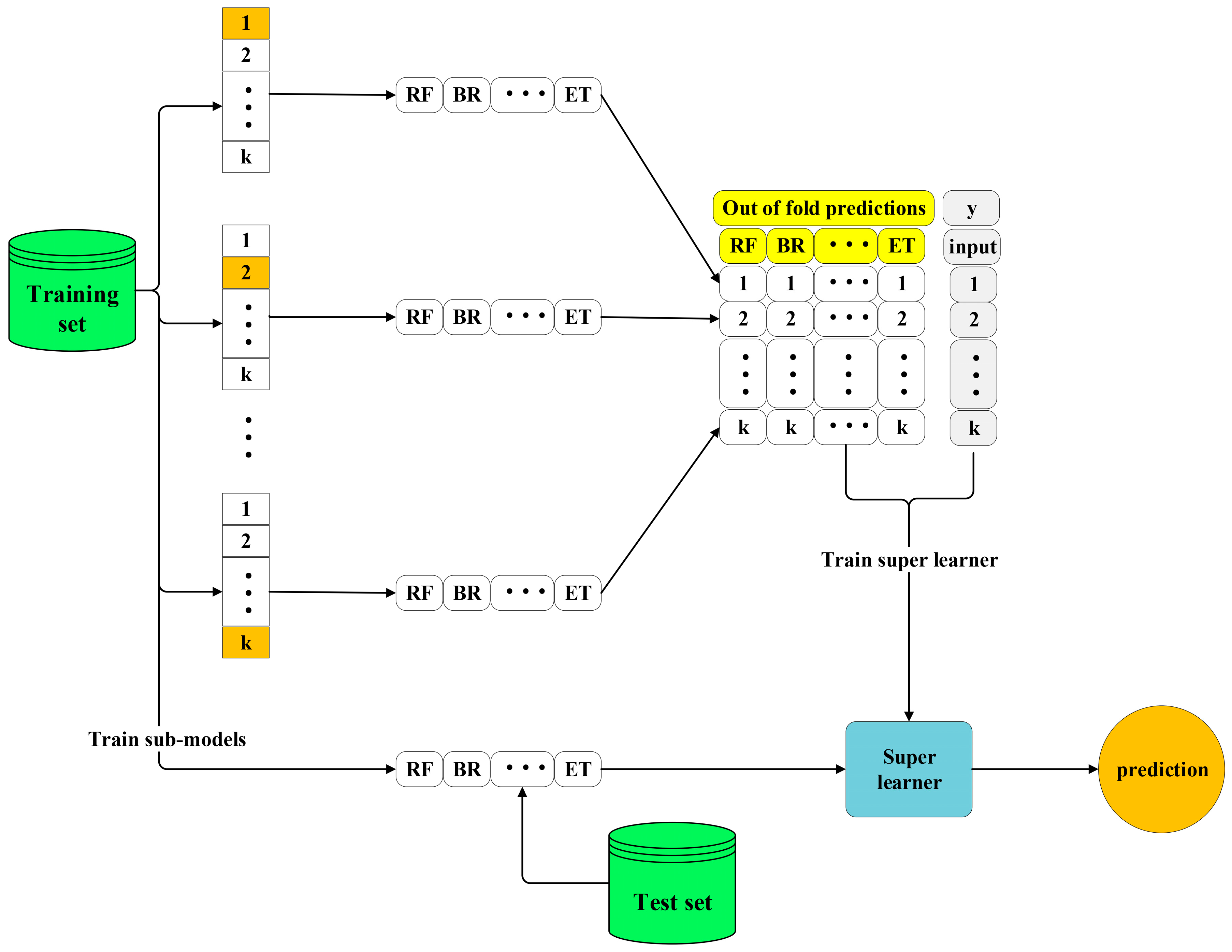
In light of the above discussion, the present study took advantage of ensemble learners and ensemble deep neural networks, including super learner, simple averaging, weighted averaging, integrated stacking, and separate stacking ensemble models, to provide an accurate model for forecasting the compressive strength of FAC. The SHAP technique was utilized to explain the best model’s predictions, rank the input features in order of relevance, and find the most important variables on the prediction of the compressive strength of FAC. This paper is structured as follows. A brief summary of the experimental database is given in Section 2. Ensemble learning models are presented in Section 3. Section 4 provides the predictions obtained with the ensemble learning models. The importance and contribution of the input variables is given in Section 5. The final section (Section 6) concludes the paper and discusses the scope for future work.

2. Experimental Database

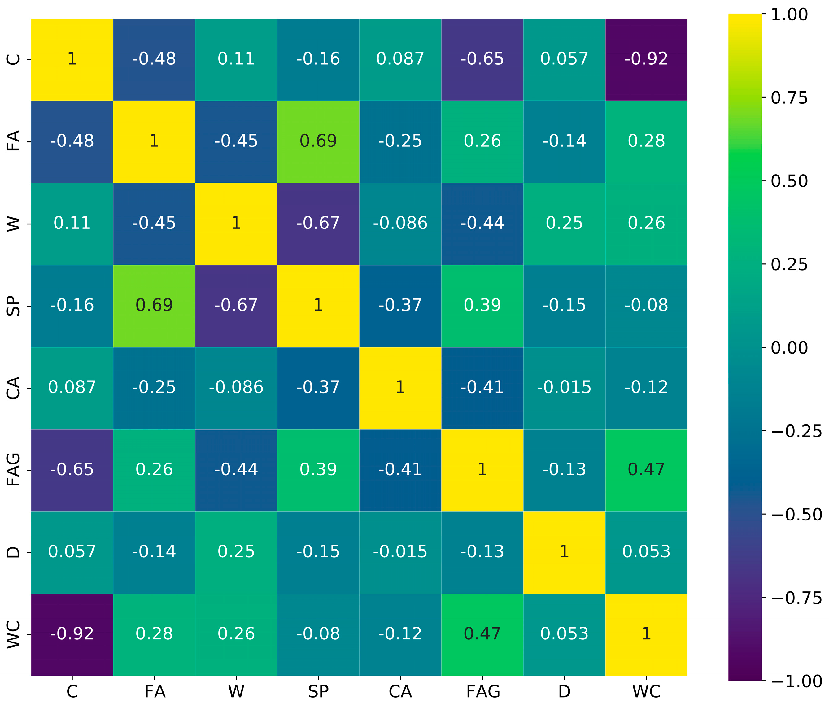
The collection and preprocessing of the dataset are the first steps in the building of an ML model. Here, the experimental database of FACs (a total of 270 samples) was obtained from the University of California, Irvine (UCI) machine learning repository [33]. The UCI machine learning repository is a library of databases, domain theories, and data providers that the machine learning community uses to test machine learning algorithms effectively. David Aha and fellow PhD students at UCI launched the archive as an online repository in 1987. Since then, it has been widely employed as a key source of machine learning resources by students, instructors, and researchers worldwide. The parameters of 270 samples include cement, fly ash, water, super plasticizer, coarse aggregate, fine aggregate, days, and water-to- cement ratio, abbreviated as C, FA, W, SP, CA, FAG, D, and WC, respectively.

Table 1. Characteristics of dataset.

	C	FA	W	SP	CA	FAG	D	WC	Strength
Unit	kg/m3	kg/m3	kg/m3	kg/m3	kg/m3	kg/m3	-	-	MPa
Mean	361.4	28.2	184.1	3.7	996.9	775.9	53.3	0.5	36.1
STD	85.5	48.4	19.3	5.9	77.3	79.9	76.1	0.1	15.0
Min	246.8	0.0	140.0	0.0	801.0	594.0	1.0	0.3	6.3
Max	540.0	142.0	228.0	28.2	1125.0	899.8	365.0	0.7	80.0

presents characteristics of the dataset and min, max, and STD are the minimum, maximum, and standard deviation of variables, respectively. A split of 20–80% of the data were used for the training and testing of models. The data were also normalized so that all values were within a range of −1 and 1. Figure 1 shows a correlation matrix of the inputs. The water-to-cement ratio did seem to correlate with the cement. The cement and fine aggregate also correlated with each other. The cement and fly ash were also correlated. Days did not seem to significantly correlate with other input parameters. Fly ash appeared to correlate well with super plasticizer. Moreover, water also negatively correlated with the super plasticizer.

3. Ensemble Model

In the current study, the compressive strength of FAC was predicted using ensemble neural network (ENN) models and the super learner approach. Deep neural networks are employed as base/basic models (sub-models) in ENN models, including simple averaging, weighted averaging, integrated stacking, and separate stacking ensemble models. However, bagging and boosting methods are utilized as sub-models in super learner ensembles. Models and their components are described in detail in the following sections.

3.1. Sub-Models

There are several hidden layers in a deep neural network (DDN). The term “deep” alludes to the more complex structure (layers and nodes), which raises the weights and bias parameters significantly, resulting in a more logical aspect mapping from the input parameters to the output. DDNs are utilized as basic learners in the ENN models. Six DDNs are used as the basic learners in this case. Using a trial-and-error approach and the GridSearchCV methodology, the number of basic learners and their attributes are determined. “Tanh” and “Adam” are also the activation functions and optimizer for all DDNs, respectively. Other attributes of the basic learners are listed in

Table 2. Characteristics of the basic models.

Sub-Models		1	2	3	4	5	6
R2 (training set)		0.94	0.95	0.97	0.97	0.98	0.98
Number of neurons	Layer 1	25	15	10	15	15	15
	Drop rate	0.01	0.02	0.01	0.01	0.01	0.01
	Layer 2	25	35	25	20	20	20
	Drop rate	-	-	-	-	-	-
	Layer 3	-	15	30	20	30	40
	Drop rate	-	-	0.01	0.01	0.01	0.01
	Layer 4	-	-	15	20	35	30
	Drop rate	-	-	-	0.02	0.02	0.02
	Layer 5	-	-	-	15	35	30
	Layer 6	-	-	-	-	20	20
	Layer 7	-	-	-	-	-	15

. These sub-models (basic models) are used to generate the basic averaging, weighted averaging, integrated stacking, and separate stacking ensemble models. As an example,

Table 3. Results of the various activation functions and optimizers for sub-model 6.

Activation Fun.	Optimizers	R2	Activation Fun.	Optimizers	R2
relu	SGD	0.759	sigmoid	SGD	0.849
relu	RMSprop	0.802	sigmoid	RMSprop	0.797
relu	Adam	0.763	sigmoid	Adam	0.806
relu	Adadelta	0.797	sigmoid	Adadelta	0.669
relu	Adagrad	0.903	sigmoid	Adagrad	0.460
relu	Adamax	0.797	sigmoid	Adamax	0.810
relu	Nadam	0.797	sigmoid	Nadam	0.805
relu	Ftrl	0.797	sigmoid	Ftrl	0.310
softplus	SGD	0.799	softsign	SGD	0.376
softplus	RMSprop	0.882	softsign	RMSprop	0.630
softplus	Adam	0.797	softsign	Adam	0.707
softplus	Adadelta	0.348	softsign	Adadelta	0.489
softplus	Adagrad	0.894	softsign	Adagrad	0.255
softplus	Adamax	0.797	softsign	Adamax	0.686
softplus	Nadam	0.797	softsign	Nadam	0.621
softplus	Ftrl	0.292	softsign	Ftrl	0.458
selu	SGD	0.706	elu	SGD	0.493
selu	RMSprop	0.602	elu	RMSprop	0.676
selu	Adam	0.696	elu	Adam	0.774
selu	Adadelta	0.580	elu	Adadelta	0.488
selu	Adagrad	0.467	elu	Adagrad	0.553
selu	Adamax	0.527	elu	Adamax	0.780
selu	Nadam	0.732	elu	Nadam	0.735
selu	Ftrl	0.310	elu	Ftrl	0.332
tanh	SGD	0.533	softmax	SGD	0.330
tanh	RMSprop	0.626	softmax	RMSprop	0.339
tanh	Adam	0.981	softmax	Adam	0.331
tanh	Adadelta	0.331	softmax	Adadelta	0.331
tanh	Adagrad	0.660	softmax	Adagrad	0.331
tanh	Adamax	0.738	softmax	Adamax	0.331
tanh	Nadam	0.744	softmax	Nadam	0.331
tanh	Ftrl	0.347	softmax	Ftrl	0.331

presents the results of the various activation functions and optimizers for sub-model 6.

3.2. Simple Averaging Ensemble

Averaging is perhaps the most common and basic combining strategy for numerical outcomes. Because of its flexibility and usefulness, the simple averaging ensemble (SAE) is one of the most commonly utilized techniques, and it is the first option in many real-world situations. Simple averaging generates the entire result by directly averaging the outputs of the sub-models. For the development of the SAE, six DDN base learners (Table 2) are taken into account. Figure 2 depicts the SAE procedure in diagram form.

3.3. Weighted Averaging Ensemble

It is easy to recognize how simple averaging can be construed as assigning equal weight to all sub-models. The weighted averaging ensemble (WEA) generates a composite output by averaging the result of each basic model with varied weights, which indicates different levels of significance. Because finding the weights is a computationally challenging task, optimization algorithms are commonly employed. Differential evolution (DE) is used in the WEA. DE is a vector-based methodology that resembles trend searching and genetic algorithms [34], due to its use of crossover and mutation. DE is a self-organizing search algorithm that does not rely on derivative data. As a result, the strategy is population-based and derivative-free. The existing population’s directional data are used by DE. Each individual of the current generation is allowed to breed by mating with other individuals of the population selected at random. Three additional members are chosen randomly from the community for each individual. As a result, a parent group of four individuals is created in order to breed an offspring. DE employs mutation to create a mutated vector linked to each population group after initialization, and then arithmetic hybridization to create a target vector in the current generation. The process for producing the changed vector distinguishes one DE scheme from another. In DE, mutation happens before crossover, whereas mutation takes place after crossover in genetic algorithms. Furthermore, whereas mutation is rarely utilized in genetic algorithms, it is used frequently in DE. The WAE-DE method is depicted in Figure 3 as a conceptual diagram.

3.4. Stacking Ensemble

Stacking ensemble is another ensemble technique that uses a meta learner to merge a large number of the basic models into a single model to offer a more precise and reliable final prediction. To put it another way, the basic models’ forecast are then combined by training a meta learner model based on the various sub-model outputs. When the meta learner is a neural network, the phrase-integrated stacking ensemble (ISE) is employed; otherwise, the separate stacking ensemble (SSE) is used. Figure 4 summarizes the stacking ensemble concept.

3.4.1. Separate Stacking Ensemble (SSE)

The support vector machine (SVM), AdaBoostRegressor, RandomForestRegressor, BaggingRegressor (BR), and GradientBoostingRegressor are employed to build SSEs with basic models (Table 2). The support vector machine was first created to classify distinct classes. A linear/non-linear transformation is employed to turn the data samples (input) into a higher-dimensional space. After that, the classification is described using a hyperplane. Because it depends on kernel functions, SVM regression is often viewed as a nonparametric approach. A kernel facilitates the search for a hyperplane in higher-dimensional space while lowering the computational cost. The Adaptive Boosting (AdaBoost) Regressor is a group of several decision trees, each of which is a weak learner and only slightly better than random guessing [35]. In order to decrease the error of the prior tree, the AdaBoost algorithm transmits the gradient of previous trees to succeeding trees. As a result, the next trees learn at each phase to aid in the establishment of a strong learner. A weighted average of each tree’s predictions yields the final prediction. Because of its flexibility, AdaBoost is more robust to outliers and noisy inputs. Bootstrap aggregation is a shortened version of bagging. It is an ensemble strategy that divides a dataset into m sample sets. Following that, each of the m samples is individually developed into m different ML models. The results of all the individual models are then combined into a single outcome via voting or averaging. RF is a bagging version that incorporates stochastic feature extraction [36]. At each phase of split selection in the creation of a decision tree, RF selects a subset of characteristics at random. The usual split selection procedure is then applied within the specified feature subset. Other methods of boosting are comparable to gradient boosting [37]. Gradient boosting, unlike AdaBoost, which consists of adding a new learner after raising the weight of weakly anticipated data, includes training a new model which is based on residual errors from the previous forecast since it requires the incremental increase or strengthening of ineffective learners.

3.4.2. Integrated Stacking Ensemble (ISE)

A neural network may be a better option as a meta learner when using deep neural networks as the basic models. In other words, a neural network is employed as a meta learner in the ISE method. The basic models can be introduced into a bigger network, and the meta learner will learn how to optimally mix the sub-models’ outputs. As the meta learner, a shallow neural network with only one hidden layer and six neurons is employed. A trial-and-error procedure is used to identify the number of neurons in the hidden layer. “Tanh” and “Adam” are the activation function and optimizer of the meta learner, respectively.

3.5. Super Learner (SL)

The SL technique is a type of ensemble method that applies stacked generalization to k-fold cross-validation, also known as the cross-validation ensemble, in which all base-models (sub-models) take the identical k-fold divides of the datasets and a meta-model is fitted to each model’s out-of-fold results. Here, base-models are SVM, AdaBoost, eXtreme Gradient Boosting (XGB), RF, BR, and ExtraTrees (ET) regressor. XGB employs the boosting strategy, in which decision trees are produced in a sequential pattern to create a strong learner. To fit the negative gradient of the preceding loss functions, each learner is joined to the total strong learner, resulting in a reduction in the overall model’s loss. RF and ET algorithms constituted a large number of decision trees. RF utilizes bootstrap replicas, which means it subsamples the inputs with replacement, whereas ET employs the entire sample. In addition, RF finds the optimum division, whereas ET picks it randomly. The procedure of the SL technique is shown in Figure 5. After splitting data to training and test sets, the training set is divided to a k-fold split (usually, k is 10). Then, each of the base-models is evaluated using the k-fold split and predictions are recorded. Additionally, each of base-models is trained using the whole training set. In addition, a meta-model is trained on the k-fold predictions result in SL creation. Then, each base-model is evaluated on a test dataset and SL uses their perdition as input to make the final prediction.

3.6. Performance Index

Model accuracy assesses how successfully the predictive model established in this research matches the input data. In examining model accuracy, the difference between the predicted and observed values is determined by calculating four metrics. The mean square error (MSE, Equation (1)), coefficient of variation (COV, Equation (3)), a-20 index (a-20, Equation (4)), and the correlation coefficient (R², Equation (2)) were selected to assess the performance of different ensemble methods.

$$\mathrm{MSE}=\frac{1}{n}{\displaystyle \sum _{i=1}^n(y_i-{\stackrel{⌢}{y}}_i}{)}^2$$

(1)

$$R^2=1-\frac{{\displaystyle \sum _{i=1}^n{(y_i-{\stackrel{⌢}{y}}_i)}^2}}{{\displaystyle \sum _{i=1}^n{(y_i-\overline{y})}^2}}$$

(2)

$$\mathrm{COV}=\frac{\sigma }{\overline{y}}$$

(3)

$$\mathrm{a}\text{-}20=\frac{m20}{n}$$

(4)

where $n$ denotes the total number of samples, $y_i$ is the observed result, ${\stackrel{⌢}{y}}_i$ is the predicted result, $\overline{y}$ is the mean of the total of samples, $\sigma$ is the results’ standard deviation, and m20 is the number of the value of the observed-to-predicted compressive strength ratio in the range of 0.8–1.2.

4. Result and Discussion

One of the most crucial characteristics of the SAE is the range of the number of basic models. For that reason, the impact of expanding the SAE to include more basic models should be explored. Using the first and second basic models (sub-models 1 and 2, Table 2), an SAE model is created and tested, after which another basic model is appended to the previous set and the model’s performance is re-evaluated. Figure 6 shows R² vs. the number of basic models. It can be seen that when the SAE model includes the basic models 1 and 2 to basic models 1–3, the R² value of the SAE models has a slight decrease. Figure 6 also shows an improvement of the accuracy from 3 to 5 sub-models. It seems the SAE model with six members converges to 0.965 since there is a marginal change in the R² value.

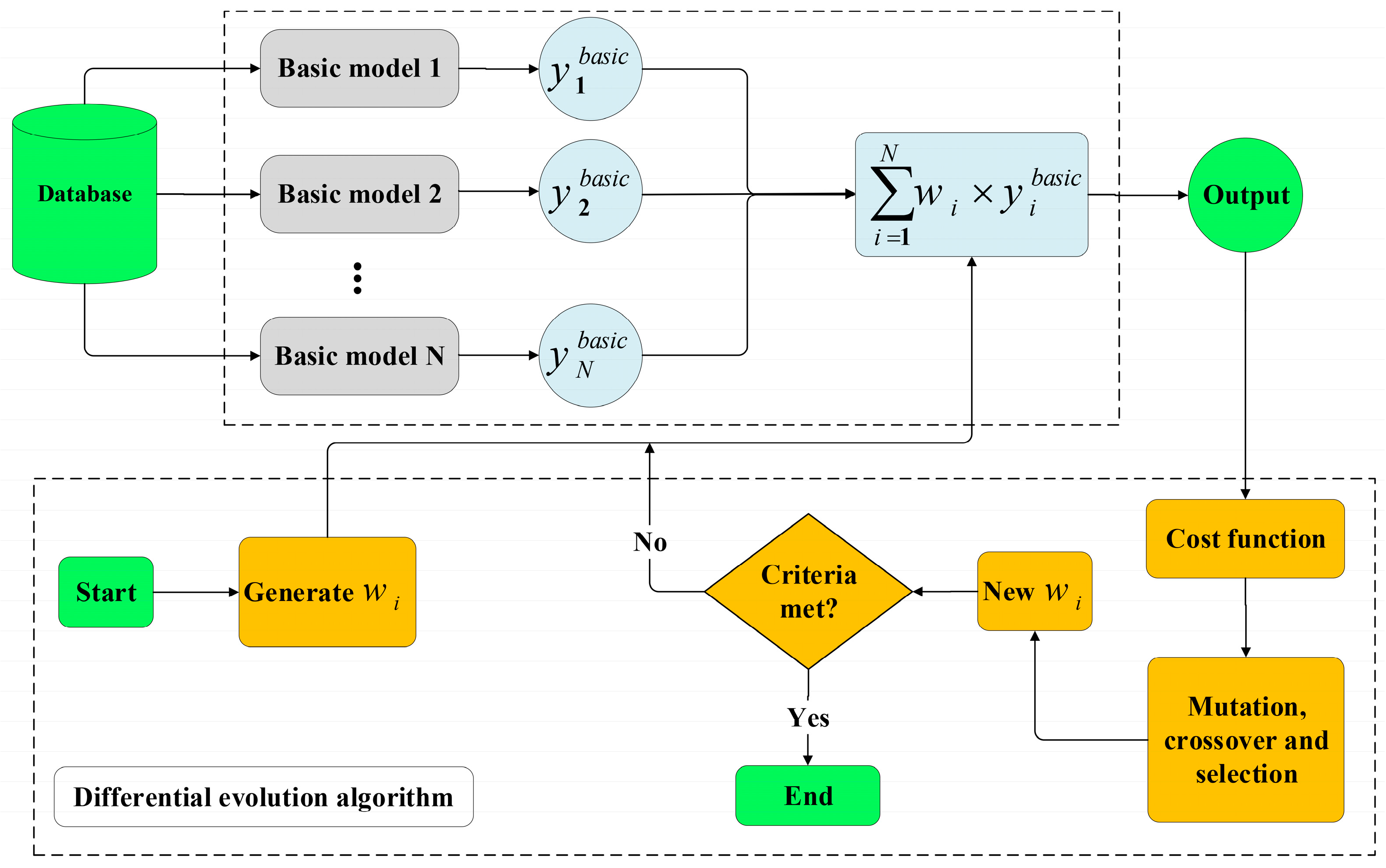
The WAE-DE is the second ensemble model. The DE algorithm is used to calculate the weight of the sub-models, as previously stated.

Table 4. Weight of the sub-models.

Sub-Models	1	2	3	4	5	6
Weight	1.11 × 10−8	2.72 × 10−8	9.88 × 10−2	2.42 × 10−1	4.01 × 10−1	2.56 × 10−1

summarizes the findings. The results reveal that basic model 5 is given higher weight. Weight values for sub-models 4 and 6 are close. For the testing phase, the R² value of the WAE-DE model is 0.973.

In

Table 5. Performance evaluation of the models.

Model		Train		Test
		MSE	R2	MSE	R2
SAE		0.005	0.966	0.0060	0.965
WAE		0.004	0.976	0.0050	0.973
SL		0.028	0.995	0.1310	0.880
ISE		0.005	0.967	0.0060	0.964
SSE	SVM	0.0043	0.973	0.0068	0.960
	AdaBoost	0.0021	0.987	0.0060	0.963
	RandomForest	0.0009	0.995	0.0041	0.976
	Bagging	0.0010	0.994	0.0049	0.971
	GradientBoosting	0.0005	0.997	0.0045	0.972

, the forecast MSE and R² values of the model for testing phase are demonstrated. For the test set, the prediction accuracy with the largest R² (0.976) and smallest MSE (0.0041) is obtained using the SSE-RandomForest algorithm among all of the given models. Meanwhile, the SSE-GradientBoosting model gives the best prediction compared to the other models, with the result of MSE and R² being 0.005 and 0.997, respectively, for the training phase. The results show that although the coefficient of determination for the SL model is very high in the learning mode, in the test mode, the model has the lowest coefficient of determination among all models. Except for the SL model, the coefficient of determination value of other models is very close, and there is a maximum difference of 1.6% between the lowest and highest value of coefficient of determination. However, in the same case, the difference for MSE reaches 65.8%.

Table 6. Properties of the measured-to-predicted values for test set.

Model		Mean	Standard Deviation	COV	a-20 Index
SAE		1.209	0.977	0.808	0.593
WAE		1.401	3.22	2.30	0.640
SL		3.030	5.672	1.872	0.10
ISE		0.962	0.394	0.409	0.648
SSE	SVM	1.113	0.955	0.858	0.593
	AdaBoost	1.704	4.489	2.63	0.537
	RandomForest	1.087	0.704	0.648	0.700
	Bagging	1.161	0.987	0.850	0.611
	GradientBoosting	1.156	1.029	0.891	0.593

shows the mean, standard deviation, COV, and a-20 index of the measured-to-predicted values for all models using test set. It can be seen that the SSE-RandomForest has the lowest COV and highest a-20 index among all models. However, ranking of the developed prediction models is difficult. A simple ranking system is utilized to analyze the efficiency of the developed models for testing datasets using the performance criteria. The total ranking index is utilized to assess the ensemble models. All models are ranked considering each indicator separately. The resulting ranking is then added together.

Table 7. Final ranking of the various models.

Model		Rank for				Total Rank
		R2	MSE	COV	a-20
SAE		5	5	3	5	18
WAE		2	4	8	3	17
SL		9	9	7	9	34
ISE		6	6	1	2	15
SSE	SVM	8	8	5	6	27
	AdaBoost	7	7	9	8	31
	RandomForest	1	1	2	1	5
	Bagging	4	3	4	4	15
	GradientBoosting	3	2	6	7	18

shows the ranking of the various ensemble models. As can be seen in the table, SSE-RandomForest ranks first, SSE-Bagging and ISE rank second, and WAE ranks third. When it came to estimating the compressive strength of FAC, both the SSE-RandomForest and SSE-Bagging algorithms performed well, although SSE-RandomForest outperformed SSE-Bagging in terms of the COV and the a-20 index.

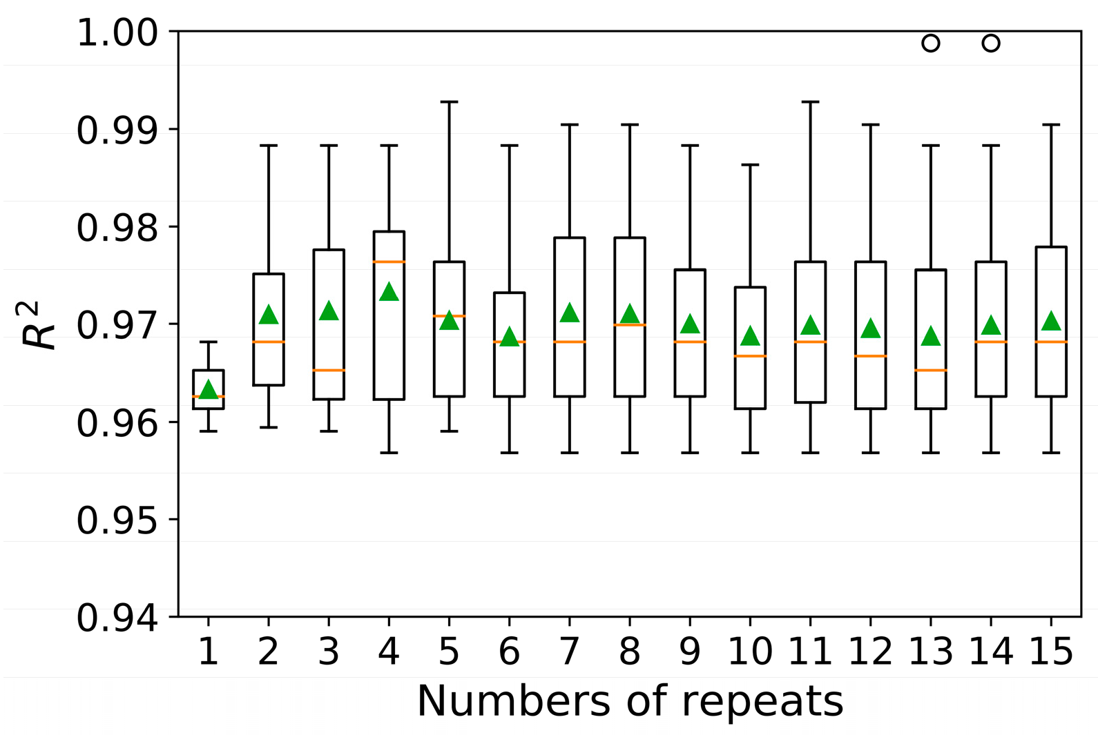
A single- run process may produce a noisy model performance assessment. Different data divisions can produce quite different findings. Repeated k-fold cross-validation is a strategy for better evaluating a machine learning model’s predicted performance. The cross-validation technique is repeated several times and returns the mean value throughout all folds from all runs. This average result should be a more accurate representation of the model’s genuine underlying mean performance on the dataset. Figure 7 shows plots of R² vs. repeats for 10-fold cross-validation. The orange line and the green triangle indicate the median and the arithmetic mean, respectively. The graph illustrates that the average fluctuates slightly around 0.97. It should be noted that for each input, the model predicts a value as an output. If the input is not in the data range, this predicted value may be associated with more error than stated.

5. SHAP (SHapely Additive exPlanations)

The black-box feature of many ML algorithms, like that of other applications, limits their usefulness. As a result, ways to describe ML models are required. In particular, there are two common reasons for describing ML models. One goal is to gain confidence in the model’s decisions. The other option is to use the model’s insights to guide human data analysis. Engineers, on the other hand, want to be directed to elements or combinations of factors that can help them understand and decrease production faults. To meet this demand, we look at the current and new tool, which is the SHAP method [38,39]. SHAP helps to understand the effect of each parameter on the prediction using game theory and Shapley values (Equation (5)).

$${\varphi }_i={\displaystyle \sum _{S\subseteq M}\frac{\left|S\right|!(M-\left|S\right|)!}{M!}}[\nu (S\cup \left\{j\right\})-\nu (S)]\hspace{0.17em}\hspace{0.17em}\hspace{0.17em}$$

(5)

where M is the players’ number, $\nu (S)$ is the contribution function, $\left|S\right|$ is coalition size, and ${\varphi }_i$ is Shapley value. For a more extensive discussion of the SHAP and the supporting proof, interested readers should refer to [38,39].

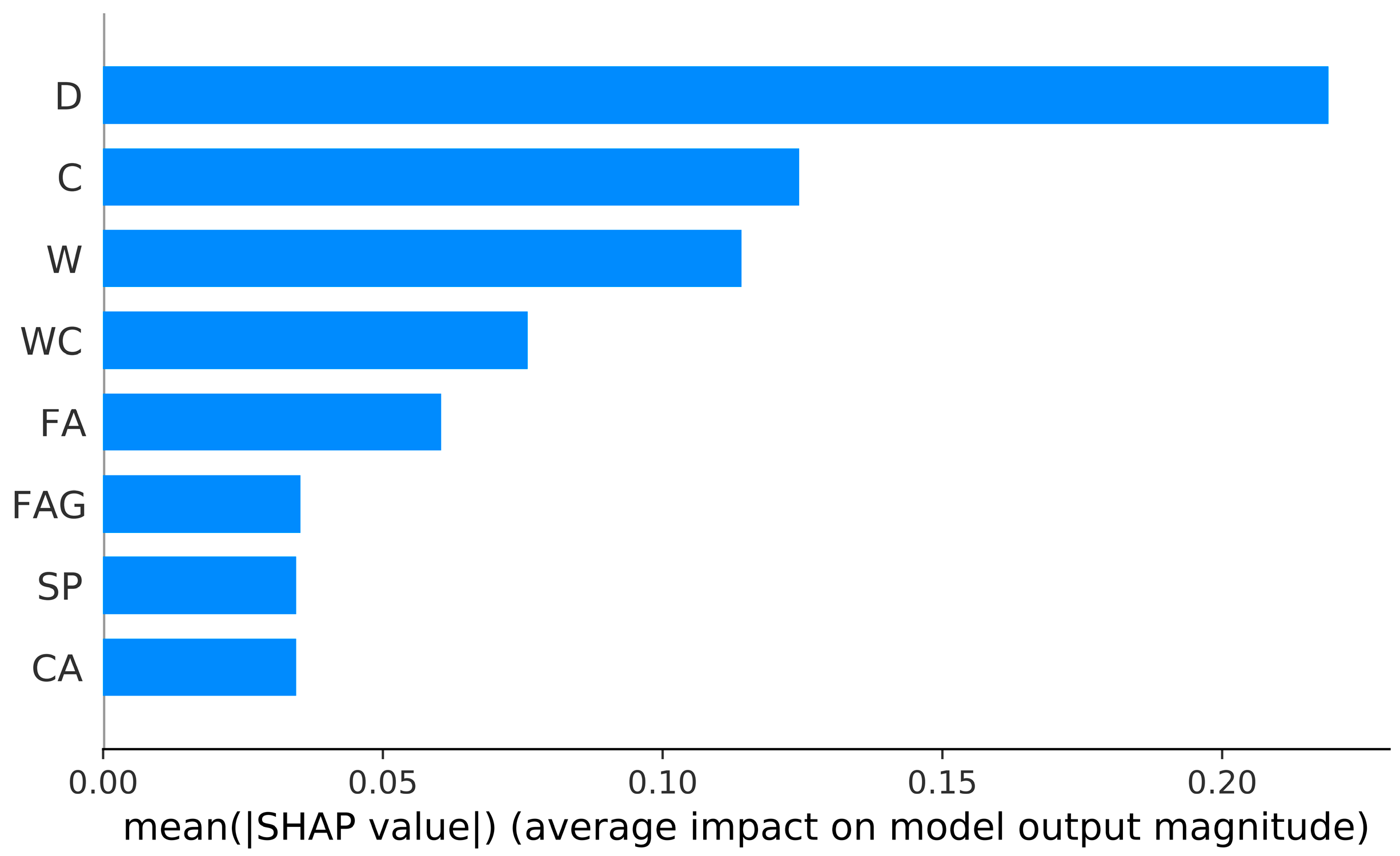
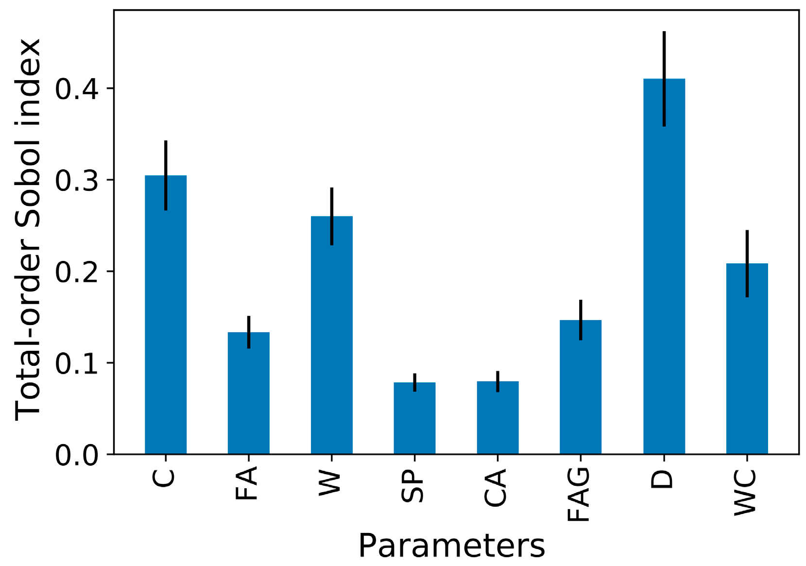
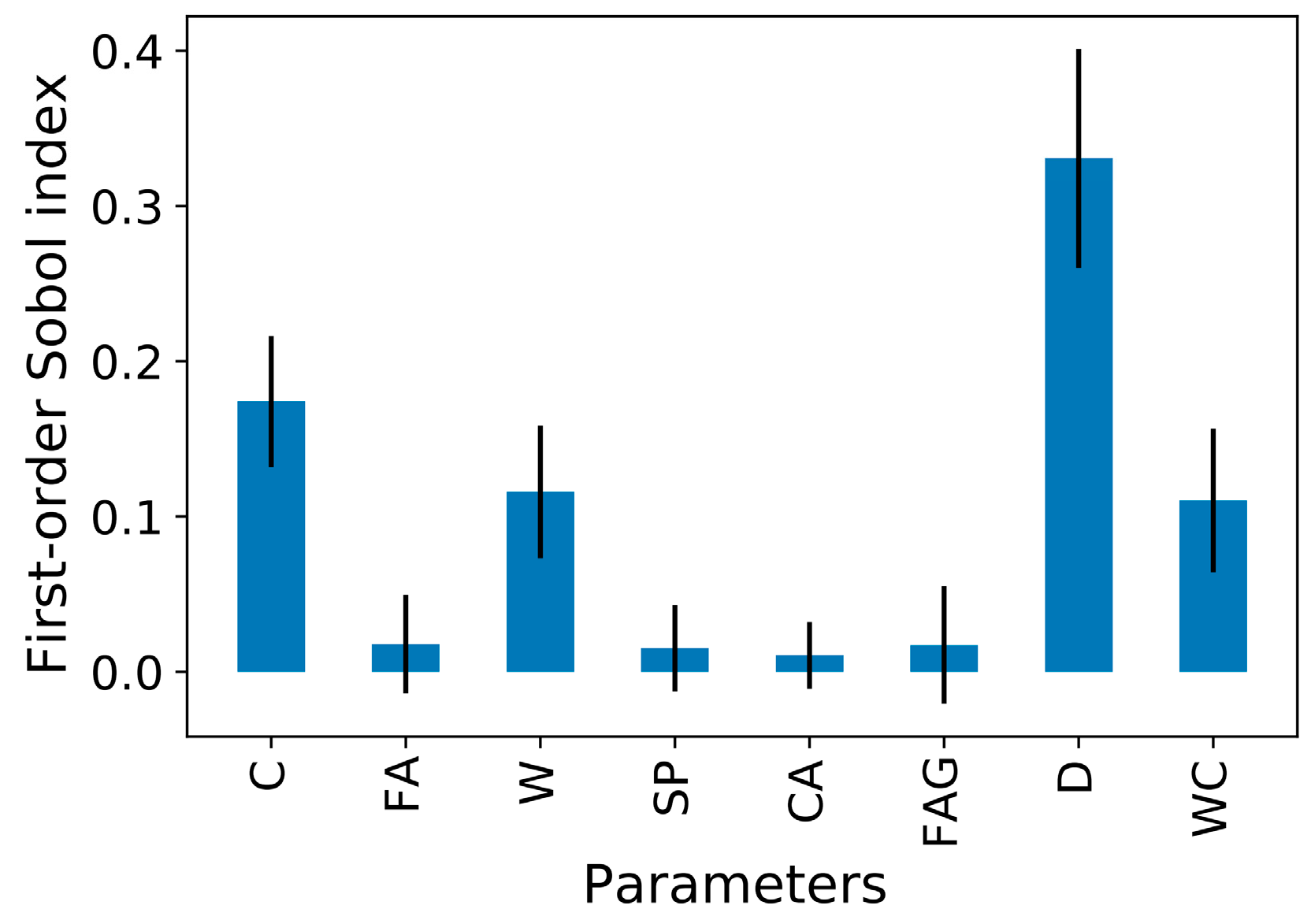
Here, the predictions of the SSE-RandomForest algorithm are explained. Figure 8 shows the feature importance using mean SHAP values in estimating the compressive strength of FAC. The y-axis presents input parameters (Section 2), and x-axis is mean Shapley values. D has the highest feature importance in the compressive strength prediction of FAC. It can be seen that the mean SHAP value of D is approximately twice the value of the second and third variables (C and W). Interestingly, FAG, SP, and CA have the lowest and almost same feature importance in the compressive strength prediction. 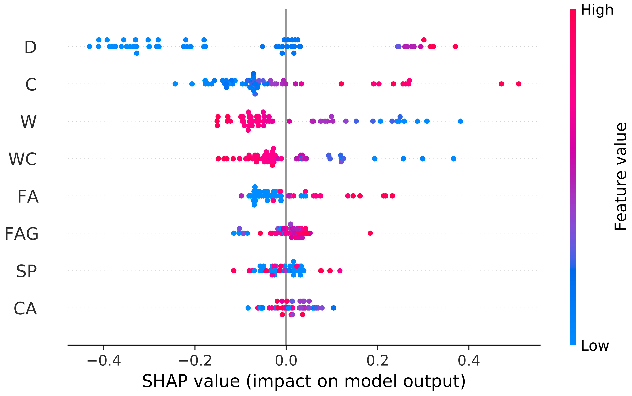Figure 9 displays the overall SHAP values. A red dot implies a positive effect, while blue represents a negative effect. The term “positive effect” refers to a growth in prediction as the variable value is increased. D and C are prominent parameters with positive influence in the compressive strength prediction. Furthermore, W and WC have negative impacts on the compressive strength of FAC. For CA, SP, and FAG, it is hard to discuss their positive/negative effect since the dots are mixed.

6. Sensitivity Analysis

The sensitivity Analysis Library (SALib) [40] in Python is used to investigate how the uncertainty in a model’s outcome can be allocated to various sources of uncertainty in its variables [41]. A bar graph of the indices is illustrated in Figure 10 and Figure 11. Figure 10 indicates that D, C, W, and WC are the dominant parameters that contribute to the compressive strength of FAC. It is interesting to note that SP and CA appear to have the same influence on the compressive strength of FAC. Figure 11 shows the first-order indices. Higher-order interactions are likely to occur if the total-order indices are significantly greater than the first-order indices. As an example, the sensitivity of the FAG and W is significantly increased by higher-order interactions between multiple variables.

7. Future Studies

The SSE-RandomForest algorithm can be used to predict the compressive strength of FAC without using too many experimental works. This study does, however, have some limitations that should be explored and addressed in future studies. Other ML algorithms should be employed to compare their accuracy in predicting outcomes. It is also suggested that the results of the durability issue for FAC be factored into the models’ execution. To compare the outcomes of different methods, it is also proposed that the use of ML algorithms be examined for FACs cured with different kinds of curing methods, such as heat curing, lime curing, and steam curing, among others. Furthermore, the dataset’s range is slightly limited. Hence, experiments, field testing, and other numerical studies using various methodologies should be used in future study to enhance data points. Despite several limitations, the findings of this study show that the method has a lot of potential in forecasting the performance of FACs. It could be a valuable tool for designing the mix proportion of FACs.

8. Conclusions

FACs replace standard Portland cement with industrial or agricultural by-product ashes as the principal binder; as a result, FAC is an eco-efficient and ecologically beneficial construction product. Compressive strength (CS) is the most significant mechanical attribute for all types of concrete. However, in the realm of design/construction, the CS of concrete at 28 days is critical. As a result, in order to save time, energy, and money, an authoritative model for forecasting the CS of the concrete is required. The objective of this study was to explore how ensemble learner (i.e., ML) techniques may be implemented to estimate the CS of FAC. Super learner, simple averaging, weighted averaging, integrated stacking, and separate stacking ensemble models were employed to predict the CS of FAC. The following are some of the inferences that can be drawn:

• The separate stacking ensemble with the random forest algorithm was more accurate in the prediction of the CS than the other approaches, as evidenced by a higher linear R² and lower mean square error.
• Other statistical indicators, including the coefficient of variation and a-20 index, have also demonstrated that a separate stacking ensemble with Bagging and integrated stacking ensemble algorithms work satisfactorily.
• Days, cement, and water contributed most to the estimation of the outcomes according to an interpretation analysis of the model’s input parameters using the SHAP method, whereas the other input variables contributed less.
• According to sensitivity results, days and cement contributed significantly, while water and water-to-cement ratio were the next highest contributors for the prediction of the output.

References

1. Possan, E.; Thomaz, W.A.; Aleandri, G.A.; Felix, E.F.; dos Santos, A.C. CO2 uptake potential due to concrete carbonation: A case study. Case Stud. Constr. Mater. 2017, 6, 147–161. [Google Scholar]
2. Barkhordari, M.S.; Tehranizadeh, M.; Scott, M.H. Numerical modelling strategy for predicting the response of reinforced concrete walls using Timoshenko theory. Mag. Concr. Res. 2021, 73, 988–1010. [Google Scholar] [CrossRef]
3. Venkateswarlu, K.; Deo, S.; Murmu, M. Effect of Super absorbent polymer on workability, strength and durability of Self consolidating concrete. Int. J. Eng. 2021, 34, 1118–1123. [Google Scholar]
4. Joel, S. Compressive strength of concrete using fly ash and rice husk ash: A review. Civ. Eng. J. 2020, 6, 1400–1410. [Google Scholar]
5. Biswas, R.; Bardhan, A.; Samui, P.; Rai, B.; Nayak, S.; Armaghani, D.J. Efficient soft computing techniques for the prediction of compressive strength of geopolymer concrete. Comput. Concr. 2021, 28, 221–232. [Google Scholar]
6. Ahmad, A.; Chaiyasarn, K.; Farooq, F.; Ahmad, W.; Suparp, S.; Aslam, F. Compressive strength prediction via gene expression programming (GEP) and artificial neural network (ANN) for concrete containing RCA. Buildings 2021, 11, 324. [Google Scholar] [CrossRef]
7. Armaghani, D.J.; Asteris, P.G. A comparative study of ANN and ANFIS models for the prediction of cement-based mortar materials compressive strength. Neural Comput. Appl. 2021, 33, 4501–4532. [Google Scholar] [CrossRef]
8. Armaghani, D.J.; Harandizadeh, H.; Momeni, E.; Maizir, H.; Zhou, J. An optimized system of GMDH-ANFIS predictive model by ICA for estimating pile bearing capacity. Artif. Intell. Rev. 2021, 54, 1–38. [Google Scholar] [CrossRef]
9. Armaghani, D.J.; Asteris, P.G.; Fatemi, S.A.; Hasanipanah, M.; Tarinejad, R.; Rashid, A.S.A.; Huynh, V.V. On the use of neuro-swarm system to forecast the pile settlement. Appl. Sci. 2020, 10, 1904. [Google Scholar] [CrossRef] [Green Version]
10. Ashrafian, A.; Taheri Amiri, M.J.; Masoumi, P.; Asadi-shiadeh, M.; Yaghoubi-chenari, M.; Mosavi, A.; Nabipour, N. Classification-based regression models for prediction of the mechanical properties of roller-compacted concrete pavement. Appl. Sci. 2020, 10, 3707. [Google Scholar] [CrossRef]
11. Paji, M.K.; Gordan, B.; Biklaryan, M.; Armaghani, D.J.; Zhou, J.; Jamshidi, M. Neuro-swarm and Neuro-imperialism Techniques to Investigate the Compressive Strength of Concrete Constructed by Freshwater and Magnetic Salty Water. Measurement 2021, 182, 109720. [Google Scholar] [CrossRef]
12. Naderpour, H.; Rafiean, A.H.; Fakharian, P. Compressive strength prediction of environmentally friendly concrete using artificial neural networks. J. Build. Eng. 2018, 16, 213–219. [Google Scholar] [CrossRef]
13. Shaban, W.M.; Elbaz, K.; Yang, J.; Shen, S.-L. A multi-objective optimization algorithm for forecasting the compressive strength of RAC with pozzolanic materials. J. Clean. Prod. 2021, 327, 129355. [Google Scholar] [CrossRef]
14. Mohammed, A.; Kurda, R.; Armaghani, D.J.; Hasanipanah, M. Prediction of compressive strength of concrete modified with fly ash: Applications of neuro-swarm and neuro-imperialism models. Comput. Concr. 2021, 27, 489–512. [Google Scholar]
15. Li, T.; Xiao, J.; Singh, A. Strength index analysis of concrete with large size recycled aggregate based on back propagation neural network. Adv. Struct. Eng. 2021, 25, 133–145. [Google Scholar] [CrossRef]
16. Imam, A.; Salami, B.A.; Oyehan, T.A. Predicting the compressive strength of a quaternary blend concrete using Bayesian regularized neural network. J. Struct. Integr. Maint. 2021, 6, 237–246. [Google Scholar] [CrossRef]
17. Korouzhdeh, T.; Eskandari-Naddaf, H.; Kazemi, R. Hybrid artificial neural network with biogeography-based optimization to assess the role of cement fineness on ecological footprint and mechanical properties of cement mortar expose to freezing/thawing. Constr. Build. Mater. 2021, 304, 124589. [Google Scholar] [CrossRef]
18. Shi-qin, H.; Hai-chao, W. Orthogonal experimental studies on mix design of high performance concrete. Ind. Constr. 2003, 33, 8–10. [Google Scholar]
19. Toufigh, V.; Jafari, A. Developing a comprehensive prediction model for compressive strength of fly ash-based geopolymer concrete (FAGC). Constr. Build. Mater. 2021, 277, 122241. [Google Scholar] [CrossRef]
20. Ahmad, A.; Farooq, F.; Niewiadomski, P.; Ostrowski, K.; Akbar, A.; Aslam, F.; Alyousef, R. Prediction of compressive strength of fly ash based concrete using individual and ensemble algorithm. Materials 2021, 14, 794. [Google Scholar] [CrossRef]
21. Farooq, F.; Czarnecki, S.; Niewiadomski, P.; Aslam, F.; Alabduljabbar, H.; Ostrowski, K.A.; Śliwa-Wieczorek, K.; Nowobilski, T.; Malazdrewicz, S. A Comparative Study for the Prediction of the Compressive Strength of Self-Compacting Concrete Modified with Fly Ash. Materials 2021, 14, 4934. [Google Scholar] [CrossRef] [PubMed]
22. Dao, D.V.; Ly, H.-B.; Trinh, S.H.; Le, T.-T.; Pham, B.T. Artificial intelligence approaches for prediction of compressive strength of geopolymer concrete. Materials 2019, 12, 983. [Google Scholar] [CrossRef] [PubMed] [Green Version]
23. Mai, H.-V.T.; Nguyen, T.-A.; Ly, H.-B.; Tran, V.Q. Investigation of ANN Model Containing One Hidden Layer for Predicting Compressive Strength of Concrete with Blast-Furnace Slag and Fly Ash. Adv. Mater. Sci. Eng. 2021, 2021, 5540853. [Google Scholar] [CrossRef]
24. Lee, S.; Park, S.; Kim, T.; Lieu, Q.X.; Lee, J. Damage quantification in truss structures by limited sensor-based surrogate model. Appl. Acoust. 2021, 172, 107547. [Google Scholar] [CrossRef]
25. Nguyen, K.T.; Nguyen, Q.D.; Le, T.A.; Shin, J.; Lee, K. Analyzing the compressive strength of green fly ash based geopolymer concrete using experiment and machine learning approaches. Constr. Build. Mater. 2020, 247, 118581. [Google Scholar] [CrossRef]
26. Huynh, A.T.; Nguyen, Q.D.; Xuan, Q.L.; Magee, B.; Chung, T.; Tran, K.T.; Nguyen, K.T. A machine learning-assisted numerical predictor for compressive strength of geopolymer concrete based on experimental data and sensitivity analysis. Appl. Sci. 2020, 10, 7726. [Google Scholar] [CrossRef]
27. Barkhordari, M.S.; Tehranizadeh, M. Response estimation of reinforced concrete shear walls using artificial neural network and simulated annealing algorithm. Structures 2021, 34, 1155–1168. [Google Scholar] [CrossRef]
28. Lieu, Q.X.; Nguyen, K.T.; Dang, K.D.; Lee, S.; Kang, J.; Lee, J. An adaptive surrogate model to structural reliability analysis using deep neural network. Expert Syst. Appl. 2022, 189, 116104. [Google Scholar] [CrossRef]
29. Ketkar, N.; Santana, E. Deep Learning with Python; Springer: Berlin/Heidelberg, Germany, 2017; Volume 1. [Google Scholar]
30. Barkhordari, M.S.; Tehranizadeh, M.; Feng, D.-C. Efficiency of Hybrid Algorithms for Estimating the Shear Strength of Deep Reinforced Concrete Beams. Period. Polytech. Civ. Eng. 2022, 66, 1–13. [Google Scholar] [CrossRef]
31. Izmailov, P.; Podoprikhin, D.; Garipov, T.; Vetrov, D.; Wilson, A.G. Averaging weights leads to wider optima and better generalization. arXiv 2018, arXiv:1803.05407. [Google Scholar]
32. Li, X.; Xiong, H.; Chen, Z.; Huan, J.; Xu, C.-Z.; Dou, D. “In-Network Ensemble”: Deep Ensemble Learning with Diversified Knowledge Distillation. ACM Trans. Intell. Syst. Technol. (TIST) 2021, 12, 1–19. [Google Scholar] [CrossRef]
33. Asuncion, A.; Newman, D. UCI Machine Learning Repository; University of California Irvine: Irvine, CA, USA, 2007. [Google Scholar]
34. Georgioudakis, M.; Plevris, V. A comparative study of differential evolution variants in constrained structural optimization. Front. Built Environ. 2020, 6, 102. [Google Scholar] [CrossRef]
35. Patil, S.; Patil, A.; Phalle, V.M. Life Prediction of Bearing by Using Adaboost Regressor. In Proceedings of the TRIBOINDIA-2018 An International Conference on Tribology, Mumbai, India, 13–15 December 2018. [Google Scholar]
36. Zhou, Z.-H. Ensemble Methods: Foundations and Algorithms; Chapman and Hall/CRC: London, UK, 2019. [Google Scholar]
37. Kumar, A.; Mayank, J. Ensemble Learning for AI Developers; Springer: Berlin/Heidelberg, Germany, 2020. [Google Scholar]
38. Lundberg, S.M.; Lee, S.-I. A unified approach to interpreting model predictions. In Proceedings of the 31st International Conference on Neural Information Processing Systems, Long Beach, CA, USA, 4–9 December 2017; pp. 4768–4777. [Google Scholar]
39. Gianfagna, L.; Di Cecco, A. Explainable AI with Python; Springer: Berlin/Heidelberg, Germany, 2021. [Google Scholar]
40. Herman, J.; Usher, W. SALib: An open-source Python library for sensitivity analysis. J. Open Source Softw. 2017, 2, 97. [Google Scholar] [CrossRef]
41. Hariri-Ardebili, M.A.; Mahdavi, G.; Abdollahi, A.; Amini, A. An RF-PCE Hybrid Surrogate Model for Sensitivity Analysis of Dams. Water 2021, 13, 302. [Google Scholar] [CrossRef]
Figure 1. Correlation matrix.
Buildings 12 00132 g001
Figure 2. Workflow of SAE procedure.
Buildings 12 00132 g002
Figure 3. Diagram of the WAE-DE hybrid algorithm.
Buildings 12 00132 g003
Figure 4. Workflow of the stacking ensemble method.
Buildings 12 00132 g004
Figure 5. Flowchart of the SL technique.
Buildings 12 00132 g005
Figure 6. Effect of the number of sub-models.
Buildings 12 00132 g006
Figure 7. Plots of R2 vs. repeats for 10-fold cross-validation.
Buildings 12 00132 g007
Figure 8. Feature importance of the compressive strength prediction of FAC.
Buildings 12 00132 g008
Figure 9. SHAP values in predicting the compressive strength of FAC.
Buildings 12 00132 g009
Figure 10. Sensitivity indices—total order index.
Buildings 12 00132 g010
Figure 11. Sensitivity indices—first-order index.
Buildings 12 00132 g011