Wind Tunnel Investigation of Twisted Wind Effect on a Typical Super-Tall Building

Abstract

This paper investigates the twisted wind effect on a typical super-tall building (500-m-tall square prism) by conducting pressure model wind tunnel tests. Two twisted wind fields (TWFs) with maximum yaw angles of approximately 30° and 20°, respectively, near the ground level were generated in the wind tunnel using a guide vane system, and the test results of wind pressure and wind load in TWFs were compared with those obtained in conventional wind fields (CWFs) with constant wind direction along the vertical axis. In particular, the distribution of extreme cladding pressure as well as the correlation and coherence of local wind loads are discussed in detail. It was observed that the mechanism of the structural dynamic responses, such as the vortex shedding, is greatly affected by TWFs. Both the distributions of mean and extreme cladding pressures in TWFs significantly differ from those in CWFs, especially on the windward and side facades. However, in terms of the amplitudes, the extreme wind pressure and the maximum wind load in TWFs do not noticeably exceed those in CWFs. This study aims to provide useful information for the wind-resistant design of future tall buildings.

1. Introduction

Tall buildings are sensitive to wind load due to their slenderness; therefore, the wind effect is one of the major concerns at the structural design stage. Most wind-resistant designs of tall buildings are based on a conventional model of the atmospheric boundary layer (ABL) winds which applies the assumption that the wind direction remains constant across the height of the structure. However, the direction of ABL winds actually varies with height due to the Coriolis force; such twisted wind flow (also referred to as veering) is known as the Ekman spiral [1]. For instance, Dyrbye and Hansen [2] reported that the wind direction at an altitude of 1 to 1.5 km differs from that near the ground by approximately 10° to 30°. Additionally, twisted wind flow may also occur because of topographical features such as mountains, that can redirect the wind flow horizontally [3,4,5]. Over the past decades, the twisted wind effect has been observed by several field measurement studies. For example, Mendenhall [6] statistically analyzed the effect of twisted wind flow caused by the horizontal temperature gradient and thermal stability. It was found that the actual wind twist angle over oceans is about 10°, whereas that over land is approximately 20°. Tamura et al. [7] conducted a long-term study of the wind characteristics in a coastal area of Japan utilizing Doppler sodars. It was observed that the wind twist angle is around 20° at altitudes between 50 and 340 m. According to wind profiler data of the wind field over a coastal area in China, recorded on 16 very windy days (synoptic wind), Liu et al. [8] reported that the variation of wind direction with height agrees well with the Ekman spiral model, and the total wind twist angle ranges from 5° to 40° over the first 1000 m above ground. Based on the synchronized measurement programs in Hong Kong using Doppler radar wind profilers and anemometers, He et al. [9] and Shu et al. [10] pointed out that the wind direction generally veers by 20–40° within the first 1.0 km above ground, and the twisted wind effect depends on the terrain condition, the wind speed, and the storm type (monsoons or typhoons). Although previous studies demonstrated that the twisted wind effect may be evident within the ABL, this effect has seldom been considered in the wind-resistant design of tall buildings. It can be intuitively understood that the wind pressure distribution on a building under the twisted wind effect in the actual ABL may significantly differ from those predicted using the conventional ABL model (i.e., whereby the wind direction remains constant across the height of the structure). Hence, failure to take into account the twisted wind effect may lead to inaccurate estimates of the wind load on tall buildings and even have a negative impact on their wind-resistance. In order to understand the wind effect on tall buildings more comprehensively, the twisted wind effect needs to be further investigated.

Boundary layer wind tunnel testing is the most common method for the experimental investigation of wind effects on tall buildings. As validated by full-scale field measurement studies in literature [11,12], wind tunnel testing can provide sufficiently accurate predictions of wind-excited structural responses. Consideration of wind twisted effects in wind tunnel tests first began with sail aerodynamics in the 1990s. By arranging guide vanes at upstream locations, Flay et al. [13,14,15] made one of the first successful attempts to simulate the twisted winds that are consistent with field measurements. Since then, guide vanes have been commonly employed for the generation of twisted winds, usually with certain modifications of their shape to serve specific purposes. Tse et al. [5] utilized a guide vane system to generate the twisted wind profiles caused by the topographic effect in Hong Kong; these profiles matched well with those obtained using a 1:2000 scale model of the city terrain. Liu et al. [16] successfully simulated two twisted wind profiles following the Ekman spiral with maximum yaw angles (i.e., horizontal variation of wind direction) of 24.2° and 14.7°, respectively. Although twisted wind flow has been simulated in several previous studies, only a few have investigated the twisted wind effect on tall buildings. Liu et al. [8] investigated the force coefficients of a super-tall building (in the shape of a square cylinder) under the twisted wind effect, although the wind pressure applied on the building was not discussed in detail. Zhou et al. [17,18] conducted both a wind tunnel test and a numerical simulation to study the twisted wind effect on a tall building. It was found that the twisted wind profile amplifies the vertical correlation and momentum exchange, resulting in a larger torsional response of the building.

In this study, the twisted wind effect on tall buildings is investigated in detail by conducting a series of wind tunnel pressure model tests. In particular, this paper further investigates the twisted wind effect focusing on aspects that have not been thoroughly discussed in the literature, including the distribution of extreme pressure on building facades as well as the correlation and coherence of local wind loads. The paper is structured as follows. Section 2 discusses the selection of the target twisted wind profiles, introduces the experimental setup for the pressure model test, and presents the method for processing the experimental data. Section 3 investigates the twisted wind effect on the wind pressure distribution, the aerodynamic characteristics, and the spatial correlation of the aerodynamic load applied at different locations of building facades. Section 4 presents the main conclusions.

2. Experimental Setups

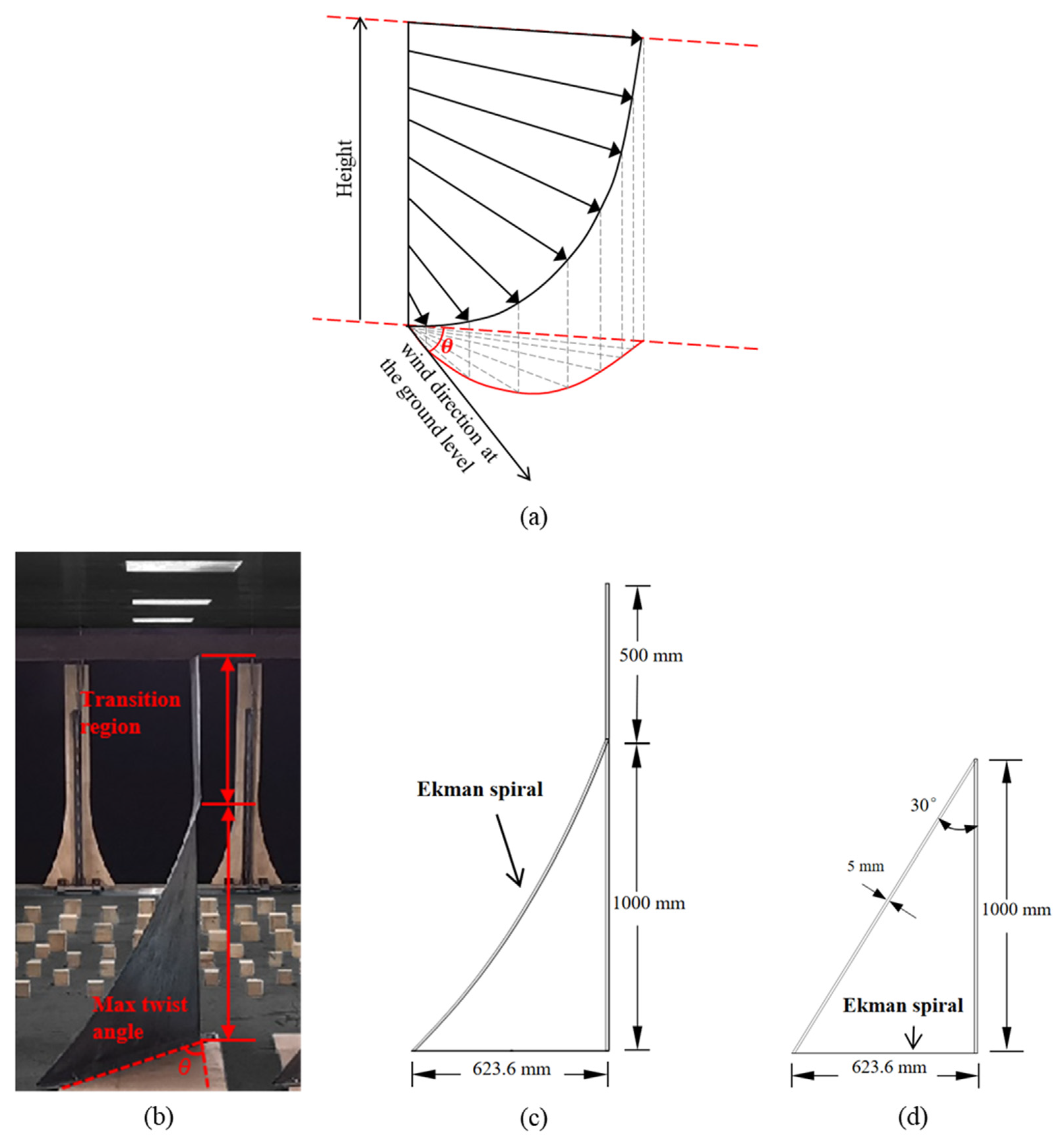
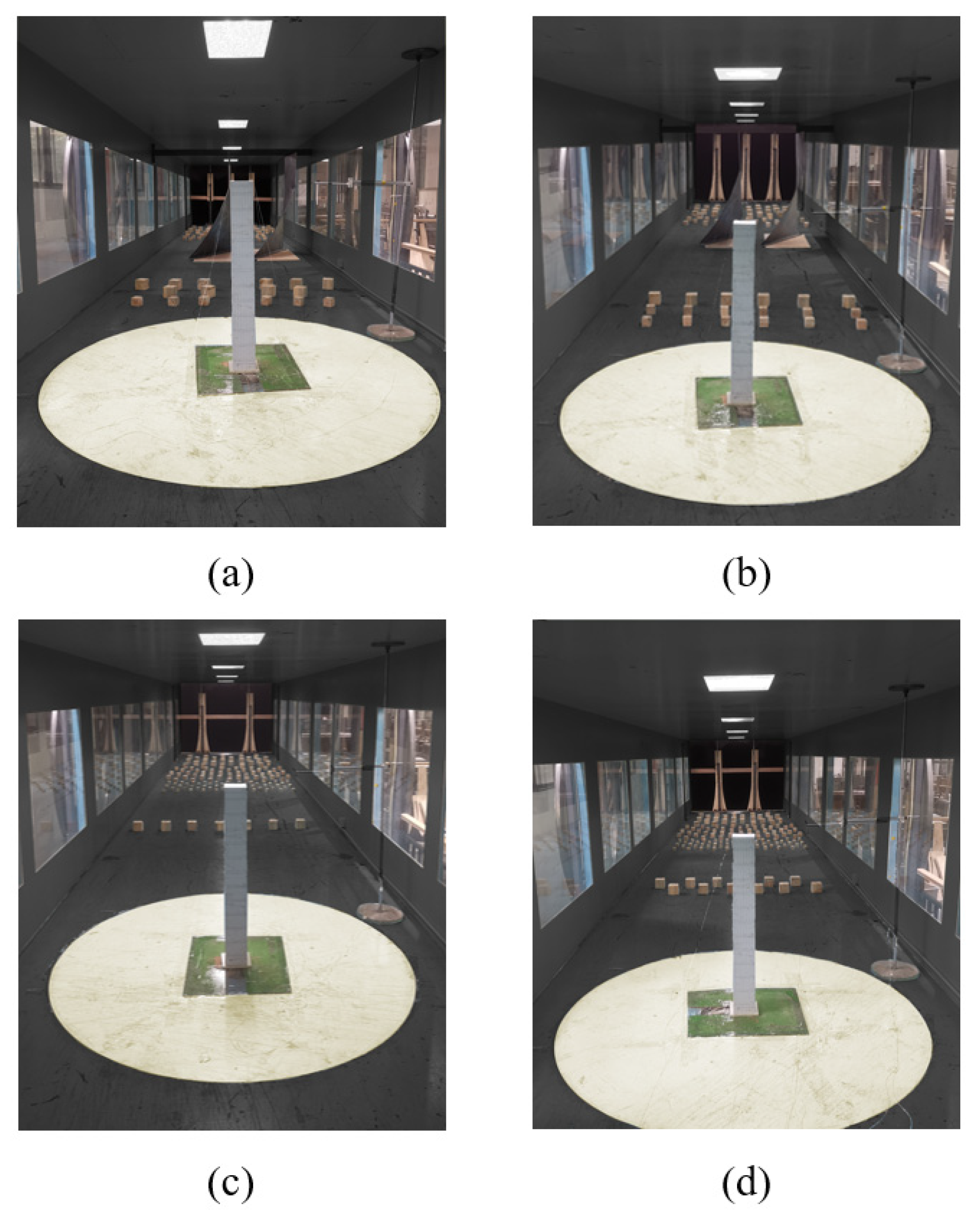
2.1. Simulation of Conventional and Twisted Wind Fields

In this study, a series of tests were conducted in the Wind Tunnel Laboratory at the School of Civil Engineering, Chongqing University. This state-of-art wind tunnel is of an open-circuit type; its test section is 2.4 × 1.8 × 15.0 (breadth × height × length, in m) in size. Two types of wind fields were simulated in the wind tunnel at a length scale of 1:500, namely, conventional wind fields (CWFs), with a constant mean wind direction along the test section on the vertical axis, and the twisted wind fields (TWFs), where the mean horizontal wind direction varies monotonically with height. Figure 1a presents the schematics of the TWF profile [17]. The CWFs were generated utilizing conventional wind tunnel setups for boundary layer winds (i.e., grids, spires, and ground roughness), whereas the TWFs were simulated by adding two identical guide vanes in the downstream area of the aforementioned conventional setup, as shown in Figure 1b. The guide vanes were made of 10-mm-thick fiberglass molded into a single piece; their locations in the wind tunnel were carefully configured to prevent the backflow from the side walls from disrupting the twisted wind field over the test section [16]. As plotted in Figure 1c, each vane has a total height of 1.5 m and consists of two sections, including a twist section ranging from ground level to 1.0 m in height and a transition section from 1.0 m to 1.5 m. The twist region has a straight leading edge, whilst its trailing edge is curved to form a guide angle that varies with the height and thus redirects the approach flow. In this study, the guide angle of the vanes follows the Ekman spiral [1]:

$$\theta \left(z\right)=arctan\left(\frac{\nu \left(z\right)}{u\left(z\right)}\right)$$

(1)

$$u\left(z\right)=u_g\left[1-e^{-z/h_E}cos\left(\frac{z}{h_E}\right)\right]-{\nu }_g{e}^{-z/h_E}\sin \left(\frac{z}{h_E}\right)$$

(2)

$$\nu \left(z\right)={\nu }_g\left[1-e^{-z/h_E}cos\left(\frac{z}{h_E}\right)\right]+u_g{e}^{-z/h_E}\sin \left(\frac{z}{h_E}\right)$$

(3)

where $z$ denotes the height in m, $\theta \left(z\right)$ denotes the guide angle in degrees at height $z$, $u\left(z\right)$ and $v\left(z\right)$ denote the along- and across-wind components of wind speed in m/s at height $z$ respectively, $u_g$ and $v_g$ denote the wind speed components at the gradient height, and $h_E$ denotes the Ekman depth in m. The gradient height is assumed to be $z=500 \mathrm{m}$ in this study and $\theta \left(0\right)-\theta \left(500\right) =30°$. On the other hand, the transition section of the guide vane is in the shape of a straight board to avoid changing the flow direction and to prevent the unfavorable eddies generated at its leading edge from reaching the building model. Readers are referred to Yuan et al. [19] for further details of the guide vane system employed in this study.

By employing the experimental setup introduced above, the wind profiles were generated in the wind tunnel following the power-law model stipulated in the structural design code AIJ-2004 [20]:

$$U\left(z\right)=U_{ref}{\left(\frac{z}{z_{ref}}\right)}^{\alpha }$$

(4)

$$I\left(z\right)=0.1{\left(\frac{z}{z_{ref}}\right)}^{-\alpha -0.05}$$

(5)

where $U\left(z\right)$ and $I\left(z\right)$ denote the longitudinal mean wind speed (in m/s) and turbulence intensity at height $z$, respectively, $U_{ref}$ and $I_{ref}$ denote the longitudinal mean wind speed and turbulence intensity at reference height $z_{ref}$, and $\alpha$ denotes the power-law exponent.

Two CWFs, referred to as CWF1 and CWF2 herein, were generated following the power-law exponents of $\alpha$ = 0.12 and $\alpha$ = 0.15, respectively. Accordingly, two TWFs with the maximum yaw angles (i.e., deviation from the mean horizontal wind direction at the reference height) of approximately 30° and 20°, referred to as TWF30 and TWF20, were generated following the same speed and turbulence intensity profiles as those of CWF1 and CWF2, respectively. Notably, due to the limitations of the experimental setup (e.g., the guide vanes need to be sufficiently separated from the side walls to avoid backflows over the test section), the two selected TWFs correspond to the most prominent twisted wind effect that was achievable in the wind tunnel. To measure the wind profiles of the CWFs and TWFs, a total of 13 discrete measurement points above the center of the turntable were selected, including 5 points ranging from 0.050 m to 0.250 m with intervals of 0.050 m, 7 points ranging from 0.350 m to 0.950 with intervals of 0.100 m, and a point at 1.000 m. A Cobra probe (Turbulent Flow Instrumentation Pty. Ltd., Tallangatta, VIC, Australia), which measures wind speeds ranging from 2 m/s to 100 m/s with an accuracy of ±0.5 m/s, was employed to assess the wind speed at each measurement point at a sampling frequency of 625 Hz for 30 s. To mitigate random measurement errors, each wind field case was measured three times, and their wind profiles were derived based on the mean values. Figure 2a–c plots the mean wind speed profiles, the turbulence intensity profiles, and the wind direction profiles (i.e., variation of yaw angle $\theta$ with height) generated in the wind tunnel, respectively. It is shown that the measured profiles of mean wind speed and turbulence intensity of both CWFs and TWFs closely match their target values with errors of less than 10%, and the measured yaw angles of TWFs at various heights only deviate from the Ekman spiral models to a reasonable extent, indicating that the wind profiles applied in this study were generated with adequate accuracy.

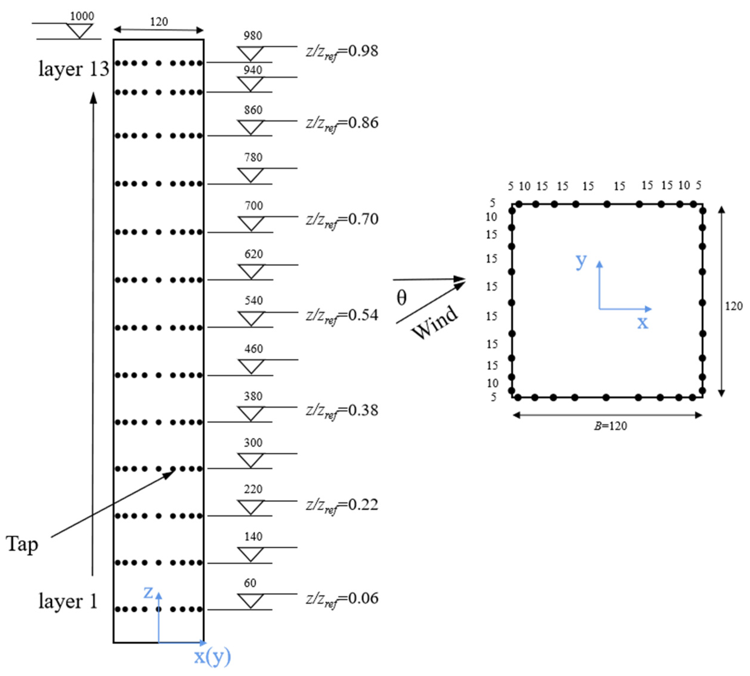
2.2. Pressure Test Model of a Super-Tall Building

To investigate the twisted wind effect on the wind load applied to a typical super-tall building, a pressure test model in the shape of a square cylinder was produced. With dimensions of 0.120 × 0.120 × 1.000 (breadth × depth × height, in m), the test model is a 1:500 replica of a building that is 60 × 60 × 500 (in m) in full-scale size. The aspect ratio of the test model is approximately 8.3, coinciding with the aspect ratio of ordinary tall buildings (e.g., [21]), which generally ranges from 7 to 9. Notably, the roof height of the building model was the same as the reference height, $z_{ref}$, of the wind profiles expressed by Equations (4) and (5). According to the size of the wind tunnel test section introduced above, the blockage ratio was 2.8% and did not exceed the threshold of 5%, which is widely accepted for the validation of experiment results. The model was made of acrylic, which provided sufficient rigidity to mitigate the wind-induced vibrations of the model itself.

The synchronous multi-pressure sensing system employed in the tests was integrated by ESP-64HD miniature electronic differential pressure scanners and a DTC Initium data acquisition unit, which supports the measurement of up to 512 channels at 1200 Hz with an accuracy of ±0.05%. To comprehensively measure the wind pressure distribution on the building envelope, a total of 468 pressure taps were installed on the four facades of the test model. Figure 3 illustrates the layout of these pressure taps, showing that there were 13 layers of taps on each facade and 9 taps in each layer. It is noted that the pressure taps were more densely distributed in the areas close to the corners, allowing them to obtain more detailed information regarding the pressure variations caused by the flow separation. In the following discussion, the case of zero wind approach angle, i.e., ${\theta }_{ref}$ = 0°, was defined as the wind at roof height (i.e., where the yaw angle equals zero in both the CWF and TWF cases) approaches perpendicularity to the windward facade of the building. A total number of 19 cases were tested by rotating the model from 0° to 180° with intervals of 10°, which is adequate to represent all wind approach angles due to the symmetry of the exterior geometry of the building (i.e., a square cylinder). Each of the 19 tests was conducted three times to reduce the random error, and the wind pressures on the building facades were sampled for 180 s at a frequency of 330 Hz each time. Figure 4 presents photos of the wind tunnel test cases with the same wind approach angle, ${\theta }_{ref}$ = 0°, in CWFs and TWFs.

3. Analysis of Test Results

3.1. Data Processing

Discussion of the wind tunnel results in this study is based on non-dimensional coefficients. By utilizing the signals of wind pressure collected from the building model, the mean and fluctuating pressure coefficients are obtained by:

$${\overline{C}}_{pij}=\frac{{\overline{p}}_{ij}-p_{\infty }}{0.5\rho U_{ref}^2}$$

(6)

$$C_{pij}^{\prime }=\frac{{\sigma }_{ij}}{0.5\rho U_{ref}^2}$$

(7)

where ${\overline{C}}_{pij}$ and $C_{pij}^{\prime }$ denote the mean and fluctuating pressure coefficients at the ($i,j$)-th pressure tap (i.e., the $i$-th layer and the $j$-th column) respectively, ${\overline{p}}_{ij}$ denotes the pressure at the ($i,j$)-th pressure tap, $p_{\infty }$ denotes the reference static pressure, $\rho$ = 1.225 kg/m³ denotes the air density, $U_{ref}$ denotes the mean wind speed at the reference height (i.e., building roof height), and ${\sigma }_{ij}$ denotes the root-mean-square (RMS) value of the fluctuating pressure record at the ($i,j$)-th pressure tap.

Meanwhile, the extreme wind pressure coefficients, including the minimum and maximum pressure coefficients, denoted by ${\check{C}}_{pij}$ and ${\widehat{C}}_{pij}$, respectively, are calculated probabilistically instead of directly adopting the values measured from the model. Following the findings by Harris [22] that the extreme wind pressure coefficients follow Type I (Gumbel) asymptotic extreme value distribution, this study employs the Cook-Mayne method [23] to calculate ${\check{C}}_{pij}$ and ${\widehat{C}}_{pij}$, which correspond to the 78% fractile of the extreme load coefficient for structural design purposes [24].

The wind forces can be calculated by integrating the wind pressures over the building facades; on this basis, the bending and torsional moments can be obtained. Figure 5 presents the definitions of the forces and moments applied to the building. The mean force coefficients are calculated as follows:

$${\overline{C}}_{FD}=\frac{{\sum }^{ }{\overline{C}}_{Pij}{A}_{ij}sin{\theta }_{ij}}{B{z}_{ref}}$$

(8)

$${\overline{C}}_{FL}=\frac{{\sum }^{ }{\overline{C}}_{Pij}{A}_{ij}cos{\theta }_{ij}}{B{z}_{ref}}$$

(9)

where ${\overline{C}}_{FD}$ and ${\overline{C}}_{FL}$ denote the mean drag and lift coefficients, respectively, $A_{ij}$ denotes the facade area represented by the ($i,j$)-th pressure tap, ${\theta }_{ij}$ denotes the wind direction at the ($i,j$)-th pressure tap, and $B$ and $z_{ref}$ denote the breadth and height of the building, respectively. Similarly, the fluctuating drag and lift coefficients, $C_{FD}^{\prime }$ and $C_{FL}^{\prime }$, are calculated by substituting $C_{Pij}$ by $C_{Pij}^{\prime }$ in Equations (8) and (9), respectively.

The mean overturning moment coefficients of the building are obtained by:

$${\overline{C}}_{MD}=\frac{{\sum }^{ }{\overline{C}}_{Pij}{A}_{ij}{z}_{ij}cos{\theta }_{ij}}{B{z}_{ref}^2}$$

(10)

$${\overline{C}}_{ML}=\frac{{\sum }^{ }{\overline{C}}_{Pij}{A}_{ij}{z}_{ij}sin{\theta }_{ij}}{B{z}_{ref}^2}$$

(11)

$${\overline{C}}_M=\sqrt{{\overline{C}}_{MD}^2+{\overline{C}}_{ML}^2}$$

(12)

where ${\overline{C}}_{MD}$, ${\overline{C}}_{ML}$, and ${\overline{C}}_M$ denote the mean moment coefficients caused by the mean drag, lift, and overall horizontal forces, respectively, and $z_{ij}$ denotes the height corresponding to the ($i,j$)-th pressure tap. Meanwhile, the mean torsional moment is calculated by:

$${\overline{C}}_{MT}=\frac{{\sum }^{ }{\overline{C}}_{pij}{A}_{ij}\left(x_{ij}\sin {\theta }_{ij}-y_{ij}\cos {\theta }_{ij}\right)}{B^2{z}_{ref}}$$

(13)

where $x_{ij}$ and $y_{ij}$ denote the coordinates of the ($i,j$)-th pressure tap in a Cartesian coordinate system ($x$, $y$) with its zero position (0, 0) at the center of the building cross-section. Through substituting $C_{Pij}$ with $C_{Pij}^{\prime }$ in Equations (10), (11), and (13), the fluctuating moment coefficients $C_{MD}^{\prime }$, $C_{ML}^{\prime }$, and $C_{MT}^{\prime }$ are obtained as well.

Furthermore, with the aim of investigating the twisted wind effect on the local wind load at a certain height, this study employs the coherence and correlation coefficients. The coherence coefficient $Coh(.)$ is expressed by:

$$Coh\left(z_i,z_j\right)=\sqrt{\frac{C_{zi,zj}^2+Q_{zi,zj}^2}{S_{zi}{S}_{zj}}}$$

(14)

where $Coh\left(z_i,z_j\right)$ denotes the coherence of the local wind load at given heights $z_i$; $z_j$, $S_{zi}$, and $S_{zj}$ are the power spectral densities of the local wind loads at the given heights, respectively, and $C_{zi,zj}^2$ and $Q_{zi,zj}^2$ are the real and imaginary parts of the cross power spectral density, respectively. On the other hand, the correlation coefficient is expressed by:

$$Cor\left(z_i,z_j\right)=\frac{Cov\left(z_i,z_j\right)}{{\sigma }_{z_i}{\sigma }_{z_j}}$$

(15)

where $Cov\left(z_i,z_j\right)$ denotes the covariance of the local wind load at given heights $z_i$, and $z_j$, and ${\sigma }_{z_i}$, and ${\sigma }_{z_j}$ denote the standard deviation of the local wind load, respectively.

3.2. Wind Pressure Distributions

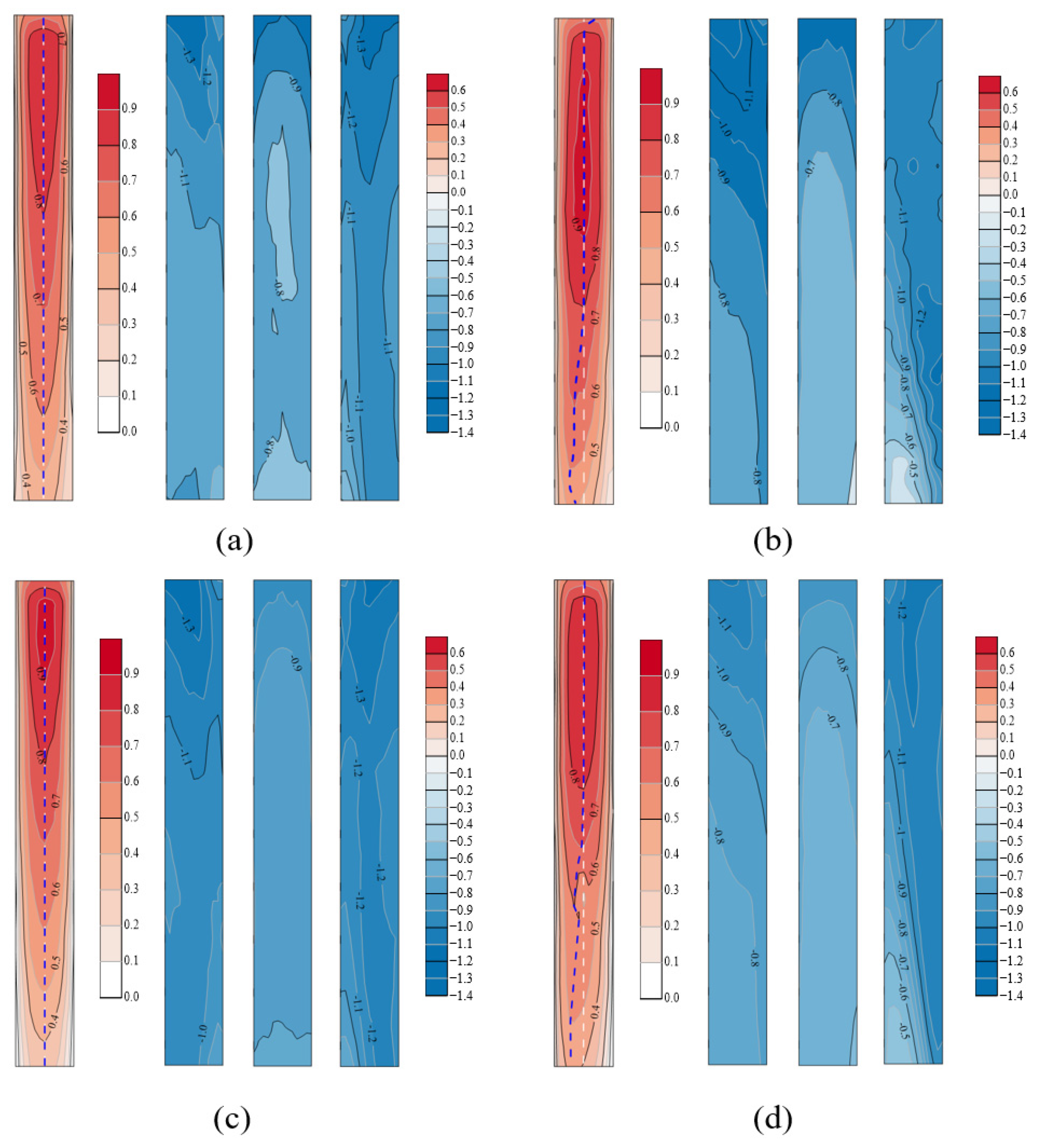
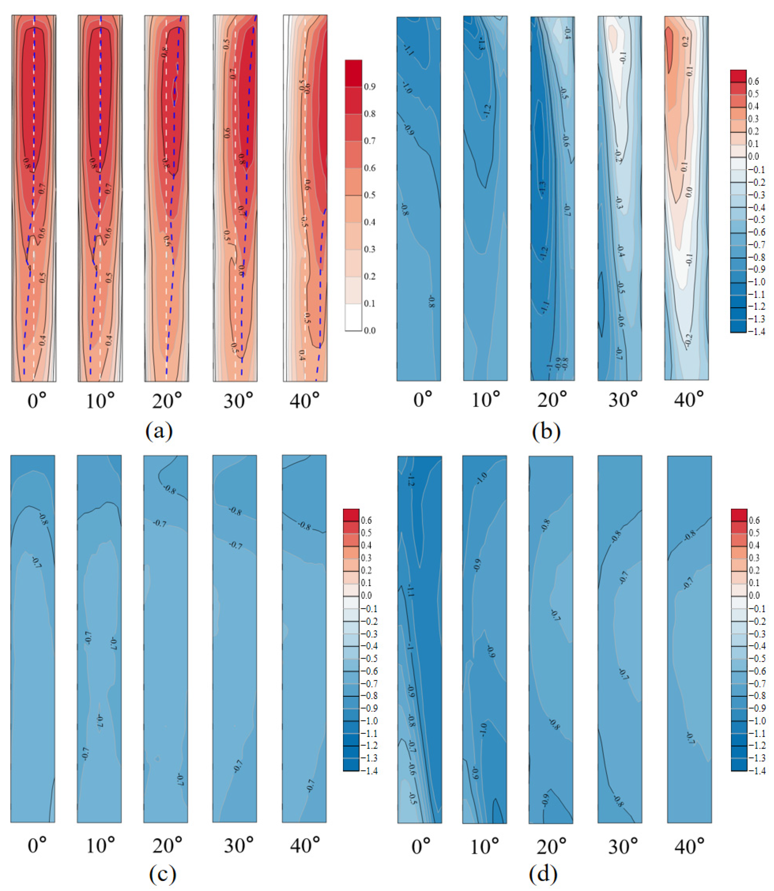
3.2.1. Mean Pressure

According to the quasi-static theorem, the mean wind pressures applied on the building facades essentially correspond to the static horizontal wind load. For the ease of discussion, each wind tunnel test case described herein is denoted by a combination of the wind field case and the wind approach angle at reference height ${\theta }_{ref}$, e.g., CWF1-0 indicates the test case of ${\theta }_{ref}$ = 0° at the building roof height in CWF1.

To investigate the twisted wind effect on the building cladding pressures, Figure 6 illustrates the ${\overline{C}}_p$ distribution in both the CWFs and the TWFs at ${\theta }_{ref}$ = 0°, i.e., CWF1-0°, CWF2-0°, TWF30-0°, and TWF20-0°. In CWF1-0°, only the windward facade is subjected to positive pressures; all the three other facades are under negative pressures. Further detailed descriptions of the ${\overline{C}}_p$ in the case CWF1-0° are omitted here because they have already been extensively discussed in the literature based on the wind tunnel test results of similar rectangular prisms, for instance, the Commonwealth Advisory Aeronautical Research Council (CAARC) standard tall building model [25]. For ease of observation and discussion, Figure 6a also plots the “ridge line” that indicates the location of the maximum ${\overline{C}}_p$ at various heights on the facade. As presented in Figure 6b, the ${\overline{C}}_p$ distribution in TWF30-0° on the upper part of windward facade is almost symmetric, whilst such symmetry dissipates as the height decreases and the ridge line of ${\overline{C}}_p$ on the lower part evidently deviates from the center line. The ${\overline{C}}_p$ distribution on the side facades also changes noticeably under the twisted wind effect. As the wind field changes from CWF1-0° to TWF30-0°, the ${\overline{C}}_p$ on the lower part of the right facade increases from [−1.1 −1.0] to [−0.9 −0.7], while the ${\overline{C}}_p$ on the left facade increases significantly from [−1.3 −0.9] to [−1.2 −0.5]. Such observations suggest that both side facades are subjected to less suction force due to the twisted wind effect, which is reasonable, because the flow separations at the leading edges are affected by changes of wind approach direction, especially on the lower parts of the side facades that correspond to a larger yaw angle. The ${\overline{C}}_p$ on the leeward facade also increases slightly, from approximately [−1.0 −0.8] to [−0.9 −0.7]. As shown in Figure 6c,d, the difference between the ${\overline{C}}_p$ distributions in CWF2-0° and TWF20-0° are similar to those in CWF1-0° and TWF30-0°, indicating that the observations of the variation pattern of the ${\overline{C}}_p$ distributions discussed above can serve as a useful reference for other TWF cases with different maximum yaw angles.

Figure 7 and Figure 8 present the distribution of ${\overline{C}}_p$ on each building facade in TWF30 and TWF20, respectively, with ${\theta }_{ref}$ varying from 0° to 40°. In TWF30, Figure 7a demonstrates that the ${\overline{C}}_p$ ridge line moves gradually toward the right as ${\theta }_{ref}$ increases, eventually going beyond the upper part of the windward facade when ${\theta }_{ref}$ reaches 40°. As for the ${\overline{C}}_p$ distribution on the right facade shown in Figure 7b, it is evident that the area under strong suction with ${\overline{C}}_p$ < −1.0 near the leading edge enlarges from a small area near the top at ${\theta }_{ref}$ = 0° to a significantly bigger area at ${\theta }_{ref}$ = 20°. Since the negative pressure on the side facade is attributed to the flow separation that occurs at the leading edge, the variation of the area under suction force implies that the shape of the separation bubble changes with ${\theta }_{ref}$. When ${\theta }_{ref}$ reaches 30°, positive pressures start to be observed on a small area near the top of the right facade, whereas the remaining part of this facade is still under negative pressures. As ${\theta }_{ref}$ continues to increase to 40°, the majority of the right facade is subjected to positive pressures, and the negative pressures only occupy the bottom area. This coincides with the observation of the ridge line of ${\overline{C}}_p$ in Figure 7a, i.e., that only the flow at low heights applies directly on the windward facade when ${\theta }_{ref}$ = 40°. Asymmetric distribution of ${\overline{C}}_p$ is also observed on the left façade, as shown in Figure 7d. As ${\theta }_{ref}$ increases from 0° to 40°, ${\overline{C}}_p$ on the majority of the left facade noticeably increases from [−1.2 −0.8] to [−0.8 −0.6], indicating that the intensity of the suction on this facade decreases with ${\theta }_{ref}$. Comparing with the other facades, the ${\overline{C}}_p$ distribution on the leeward facade does not noticeably change with ${\theta }_{ref}$. Similar observations are illustrated in Figure 8 under TWF20, and therefore, a detailed description of this figure is omitted to avoid repetition.

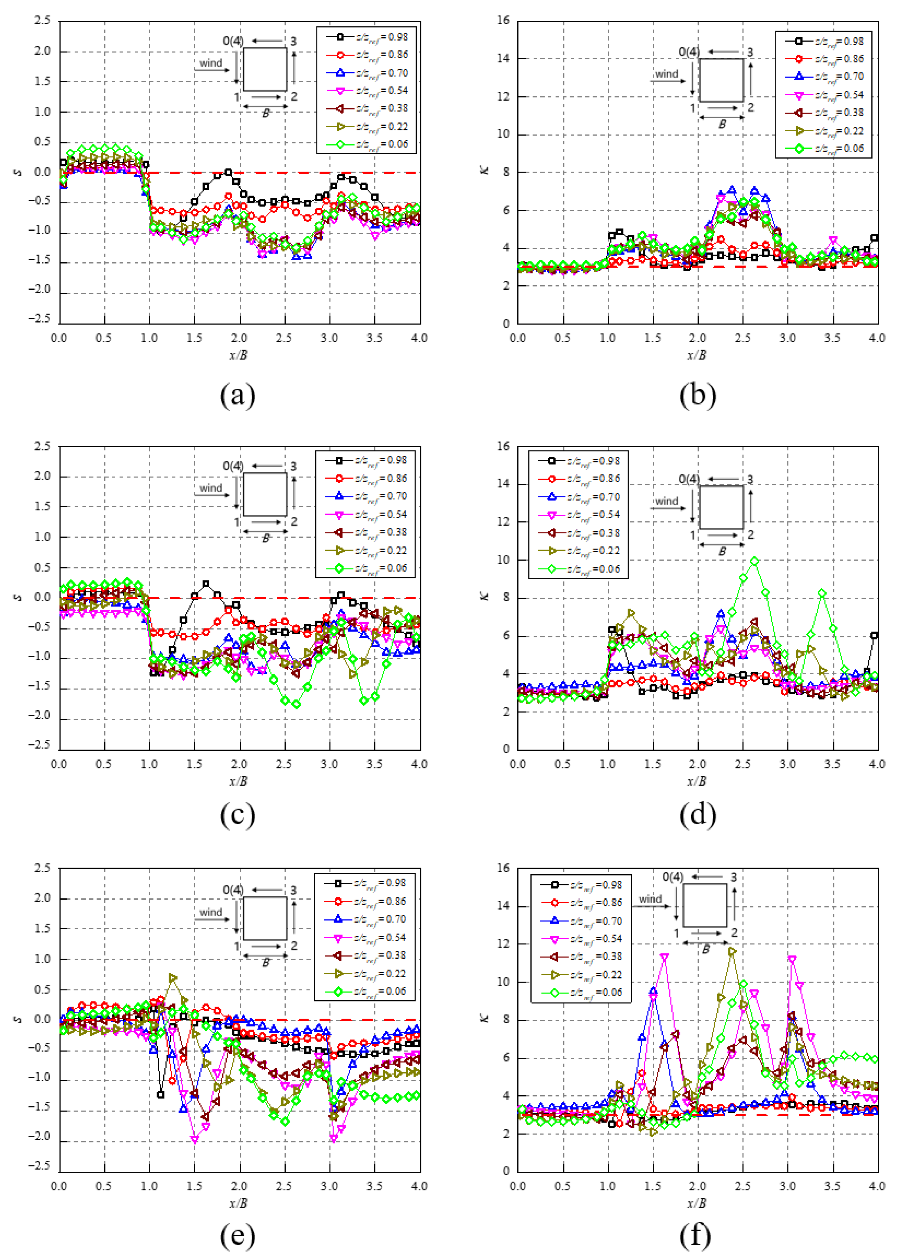
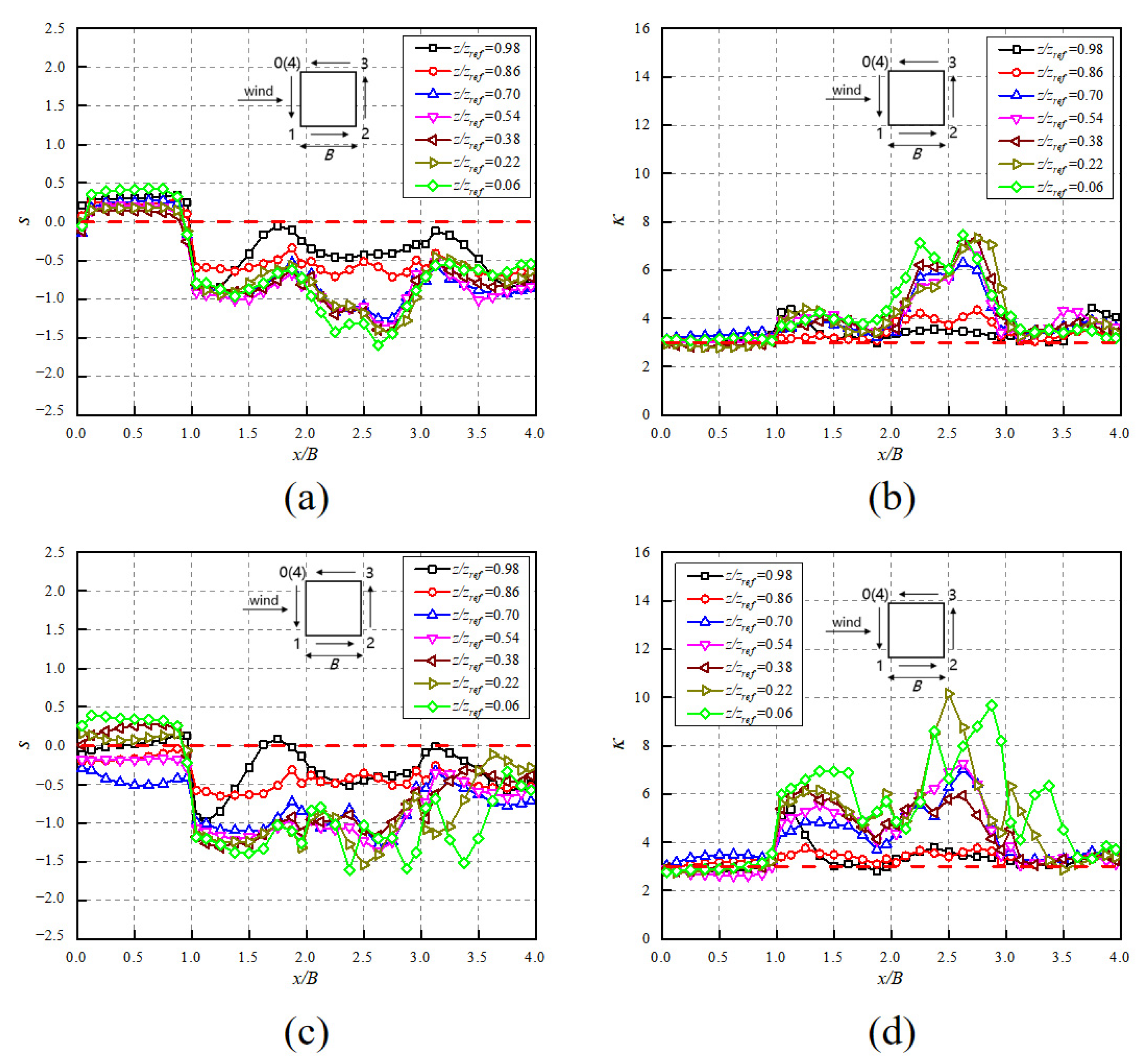
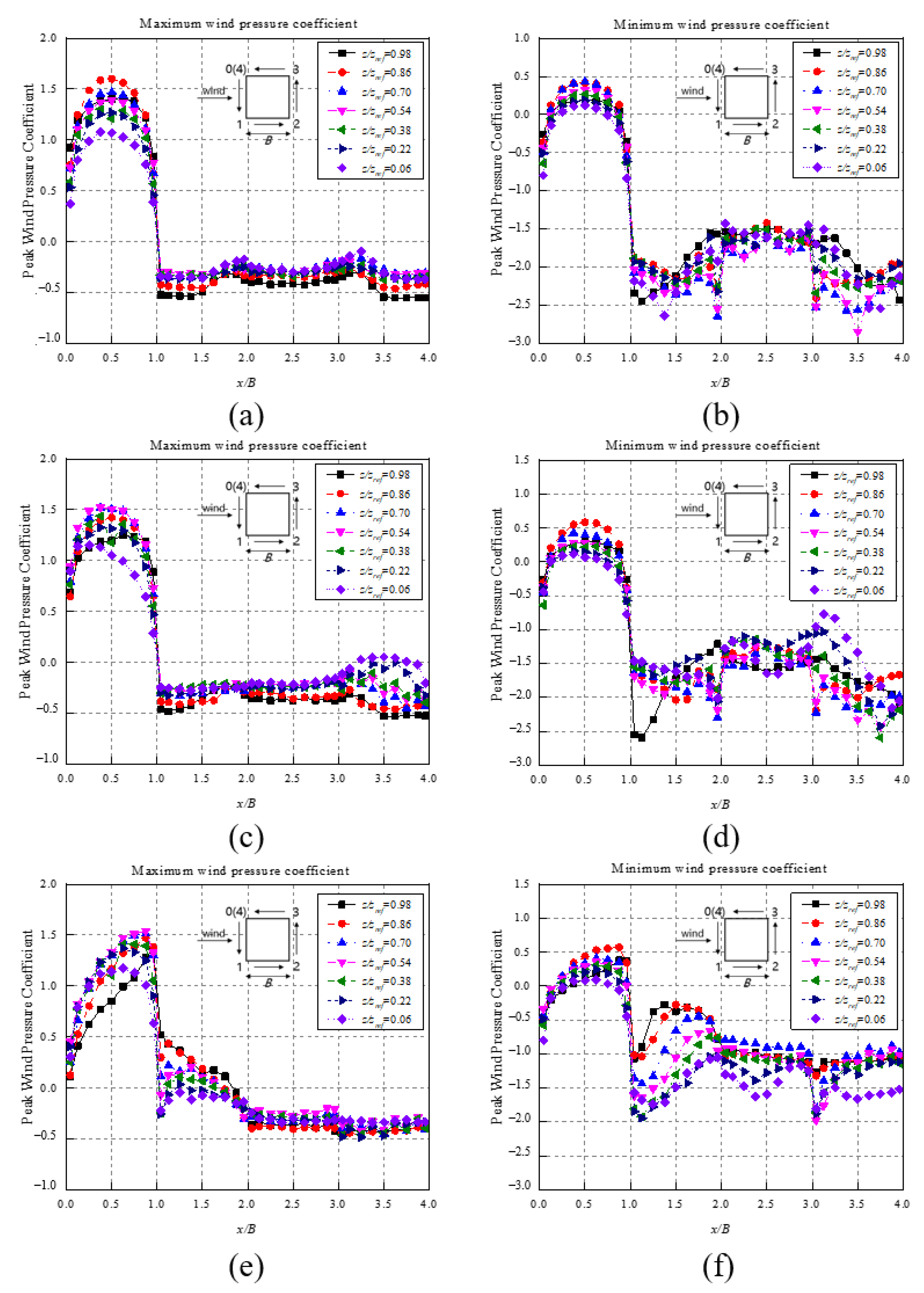
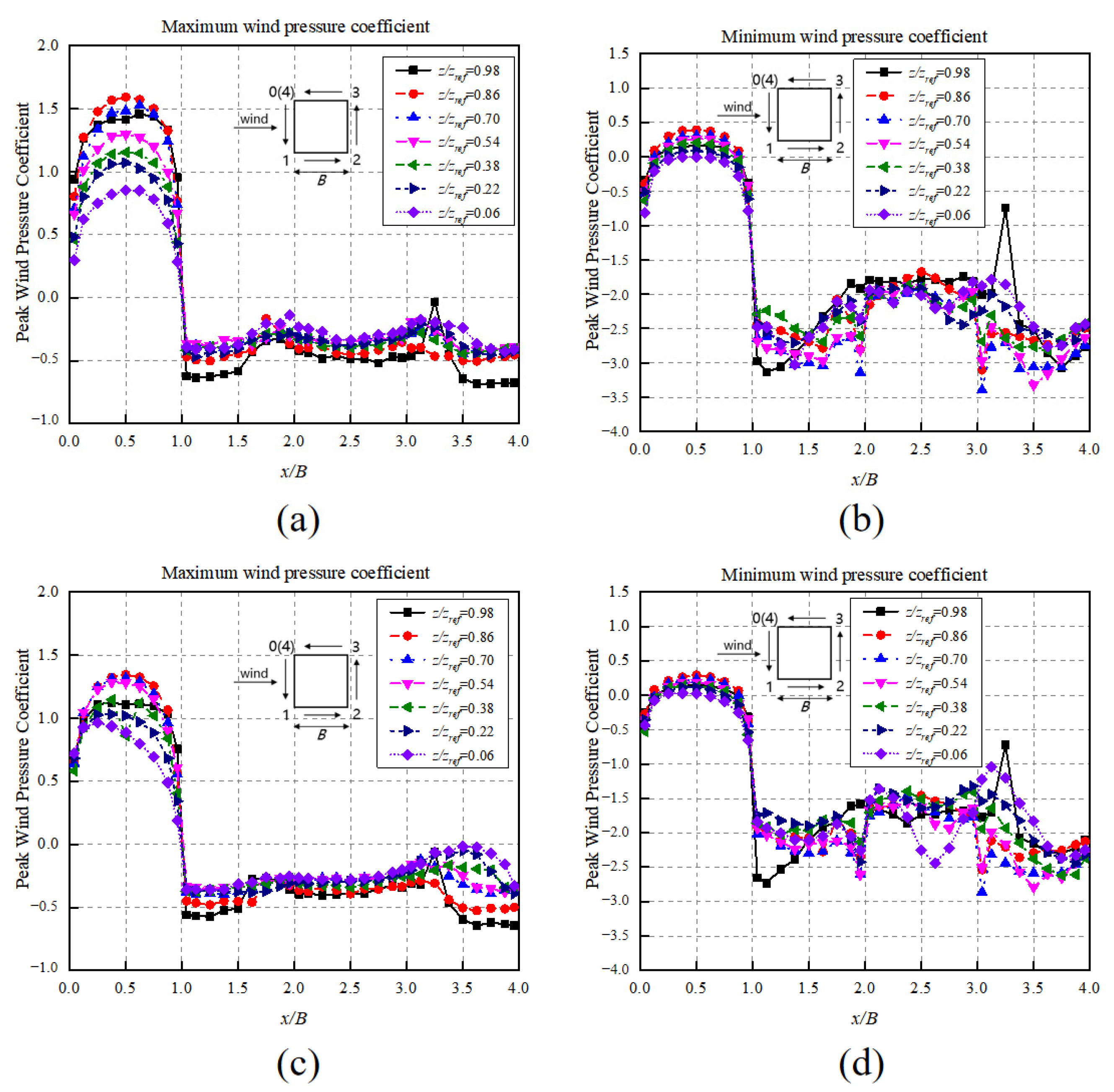
3.2.2. Extreme Pressure

The fluctuating component of wind pressure corresponds to the dynamic force applied to the building. In particular, extreme wind pressure is a major concern in the design of building envelopes, because excessive pressures may lead to envelope failure. It is worth noting that most of the wind standards and codes of practice calculate the extreme wind pressures under the assumption that the probability density function (PDF) of wind pressure is Gaussian, so that the extreme pressure can easily be calculated using only the mean and the standard deviation of the wind pressure. However, such an assumption may not be applicable to the wind pressure on bluff bodies due to the flow patterns such as separation, which lead to a non-Gaussian distribution of wind pressure on the side and leeward facades. Therefore, in order to calculate the extreme pressure, it is a necessity to first investigate the Gaussianess of the pressure on the building facades.

Gaussianess can be quantified by skewness and kurtosis, denoted by $s$ and $\kappa$, respectively; a Gaussian distribution corresponds to $s$ = 0 and $\kappa$ =3. Figure 9 illustrates the $s$ and $\kappa$ of the pressure records at different layers on the building facades in CWF1-0°, TWF30-0°, and TWF30-30°. Notably, TWF30-0° and TWF30-30° are selected herein for comparison with CWF1-0°, because they correspond to a yaw angle of 0° at the roof and ground levels, respectively. In CWF1-0°, as presented in Figure 9a,b, the wind pressure on the windward facade (0 < x/B < 1, as indicated in the figure) generally follows Gaussian distribution with $s$ = 0 ± 0.4 and $\kappa$ = 3 ± 0.2. Meanwhile, evident non-Gaussian features are observed on the side (1 < x/B < 2 and 3 < x/B < 4) and leeward (2 < x/B < 3) facades, where the values of $s$ are mostly lower than –0.5, and those of $\kappa$ are mostly higher than 4.0. As shown in Figure 9c–f, the values of $s$ and $\kappa$ of the pressures on the windward facade fluctuate around 0 and 3, respectively, indicating that the pressure on the windward facade still follows Gaussian distribution under the twisted wind effect. The pressure on the side and leeward facades in both TWF30-0° and TWF30-30° demonstrates prominent non-Gaussian features, given that $s$ and $\kappa$ deviate considerably from 0 and 3, respectively. The variations of $s$ and $\kappa$ on these facades near the building top ($z/z_{ref}$ > 0.7) in TWF30-0° are similar to those in CWF1-0°, which is reasonable, because the winds applied on the upper section of the building approach from roughly the same direction in both TWF30-0° and CWF1-0°. However, the variations of $s$ and $\kappa$ on the lower parts ($z/z_{ref}$ ≤ 0.54) of the side and leeward facades are considerably different in TWF30-0° and CWF1-0°. For instance, the $s$ and $\kappa$ at x/B = 3.375 in TWF30-0° are more than twice those in CWF1-0°, implying that the flow field around the building at the lower heights considerably changes due to the twisted wind effect. On the other hand, the variations of $s$ and $\kappa$ in TWF30-30° on the side facades are significantly different from those in CWF1-0°, even at the bottom layer ($z/z_{ref}$ = 0.06), where the yaw angles of the wind flow are similar. At the layers $z/z_{ref}$ ≤ 0.70, both $s$ and $\kappa$ change abruptly without a clear pattern; the most evident the non-Gaussianess is observed at x/B around 1.5, 2.5, and 3.0. As expected, the variations of $s$ and $\kappa$ under CWF2-0° and TWF20-0°, as illustrated in Figure 10, are similar to those presented in Figure 9a–d, as discussed above.

Utilizing the Cook-Mayne method, the maximum and minimum pressure coefficients, denoted by ${\widehat{C}}_p$ and ${\check{C}}_p$, respectively, within a 10-min time interval at full scale are calculated following the four-step procedure below:

• We selected ten data segments with a duration of 10 min in full-scale, and ranked the absolute values of the extreme wind pressure coefficient of each segment in ascending order.
• We used Equations (16) and (17) to calculate the mode and dispersion:

  $$u={\displaystyle \sum }_{i=1}^{10}{a}_i{X}_i$$

  (16)

  $$1/a={\displaystyle \sum }_{i=1}^{10}{b}_i{X}_i$$

  (17)

  where $X_i$ is the wind pressure coefficient obtained in the previous step, and the values of $a_i$ and $b_i$ are taken in accordance with

  Table 1. Coefficients $a_i$ and $b_i$ for the Cook-Mayne method.

  $\mathit{i}$	1	3	2	4	5	6	7	8	9	10
  $a_i$	0.22	0.16	0.13	0.11	0.096	0.081	0.067	0.054	0.042	0.029
  $b_i$	−0.35	−0.091	−0.019	0.022	0.049	0.066	0.077	0.083	0.084	0.078

  .
• The extreme value is calculated using Equation (18):

  $$x_e=u+y/a$$

  (18)

  where y = 1.4 corresponding to a transcendence probability of 22%.
• We take $x_e$ as ${\widehat{C}}_p$ or $-x_e$ as ${\check{C}}_p$.

Figure 11a–f illustrates the variations of ${\widehat{C}}_p$ and ${\check{C}}_p$ in CWF1-0°, TWF30-0°, and TWF30-30°, respectively. As shown in Figure 11a, the maximum ${\widehat{C}}_p$= 1.55 in CWF1-0 occurs at x/B = 0.5 at the layer $z/z_{ref}$ = 0.86 on the windward facade, indicating that the stagnation point is close to this location. Comparing with CWF1-0°, Figure 11c shows that the values of ${\widehat{C}}_p$ at the layer $z/z_{ref}$ = 0.86 in TWF30-0° are slightly lower, and the stagnation point appears to be at a lower position, because the maximum ${\widehat{C}}_p$ = 1.50 is observed at the layer $z/z_{ref}$ = 0.70 instead of 0.86. At the bottom layer, $z/z_{ref}$ = 0.06, the maximum wind pressure becomes noticeably higher under the twisted wind effect; in particular, the ${\widehat{C}}_p$ value near the leading edge at x/B = 0.04 increases from 0.4 in CWF1-0° to 0.9 in TWF30-0°. On the side facade, 3 < x/B < 4, the ${\widehat{C}}_p$ values of the bottom two layers, i.e., $z/z_{ref}$ = 0.06 and 0.22, generally increase to nearly zero. Similar to Figure 11c, Figure 11e also shows that the maximum ${\widehat{C}}_p$ slightly decreases from 1.55 in CWF1-0° to 1.50 in TWF30-30°, and it is found at a lower layer $z/z_{ref}$ = 0.54 instead of 0.86, which implies a lower location of the stagnation point. At all layers except $z/z_{ref}$ = 0.06, i.e., the locations of the maximum ${\widehat{C}}_p$ on the windward facade, shift from the middle (x/B = 0.5) in CWF1-0 to the edge in TWF30-30°, and the maximum ${\widehat{C}}_p$ values at the upper layers $z/z_{ref}$ > 0.54 are all found at x/B = 0.985. The ${\widehat{C}}_p$ values on the side facade 1 < x/B < 2 at all layers in TWF30-30° are higher than those in CWF1-0°, and those at layers $z/z_{ref}$ > 0.38 even exceed zero, which indicates that positive pressure is occurring on this facade. The ${\widehat{C}}_p$ values on the other facades 2 < x/B < 4 in TWF30-30°, however, generally remain at the same amplitudes, ranging from −0.5 to −0.2, as in CWF1-0°.

On the other hand, the ${\check{C}}_p$ values in TWF30-0° and TWF30-30° also differ significantly from those in CWF1-0°. Figure 11d shows that the values in TWF30-0° on the windward facade 0 < x/B < 1 are generally the same as those in CWF1-0°, except for those at the layer $z/z_{ref}$ = 0.86, which increase by approximately 0.3. On the side facade 1 < x/B < 2, the ${\check{C}}_p$ values near the leading edge at 1 < x/B < 1.375 slightly increase at the layers $z/z_{ref}$ < 0.98. The ${\check{C}}_p$ values on facades 2 < x/B < 4 are generally the same as those in CWF 1-0°, except for those at 3 < x/B < 3.5 at the bottom two layers $z/z_{ref}$ = 0.06 and 0.22, which increase by about 0.5. In TWF30-30°, as shown in Figure 11f, the ${\check{C}}_p$ values are generally similar to those in CWF1-0°, whilst the values at x/B > 0.5 at the top two layers $z/z_{ref}$ = 0.86 and 0.98 increase slightly. Comparing with CWF1-0°, the ${\check{C}}_p$ values in TWF30-30° on the side and leeward facades 1< x/B < 4 generally increase by 1.0 to 1.5, suggesting that a weaker suction force is applied on these facades under the twisted wind effect.

As plotted in Figure 12, the variations of ${\widehat{C}}_p$ and ${\check{C}}_p$ under TWF2-0° and TWF20-0° are similar to those presented in Figure 10a–d. In general, the absolute values of the peak pressure coefficients under the twisted wind effect are lower than those under the conventional wind field, suggesting that less suction is applied on the facades, which is favorable to a wind-resistant design.

3.3. Characteristics of Wind Loads under Twisted Wind Effect

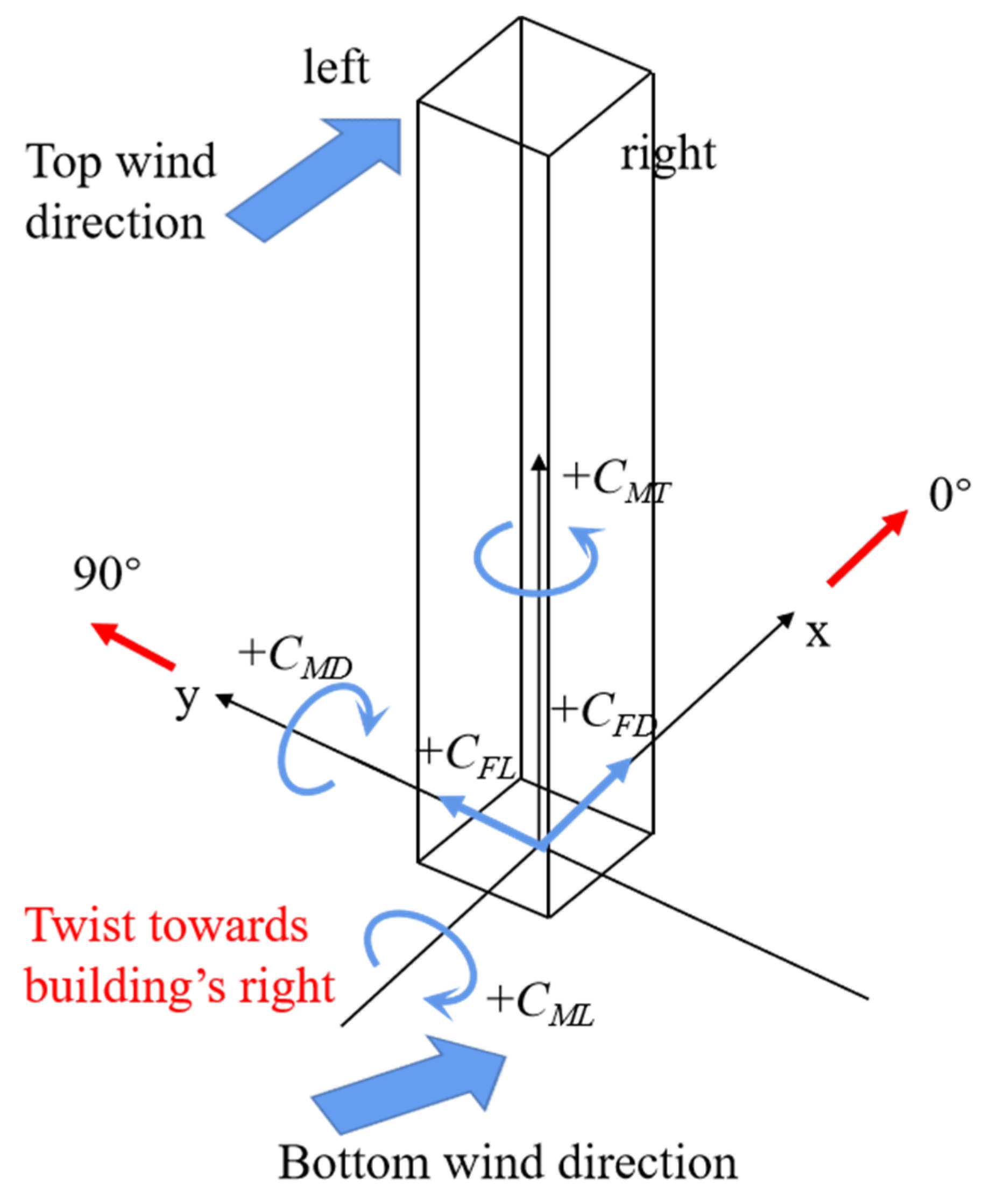
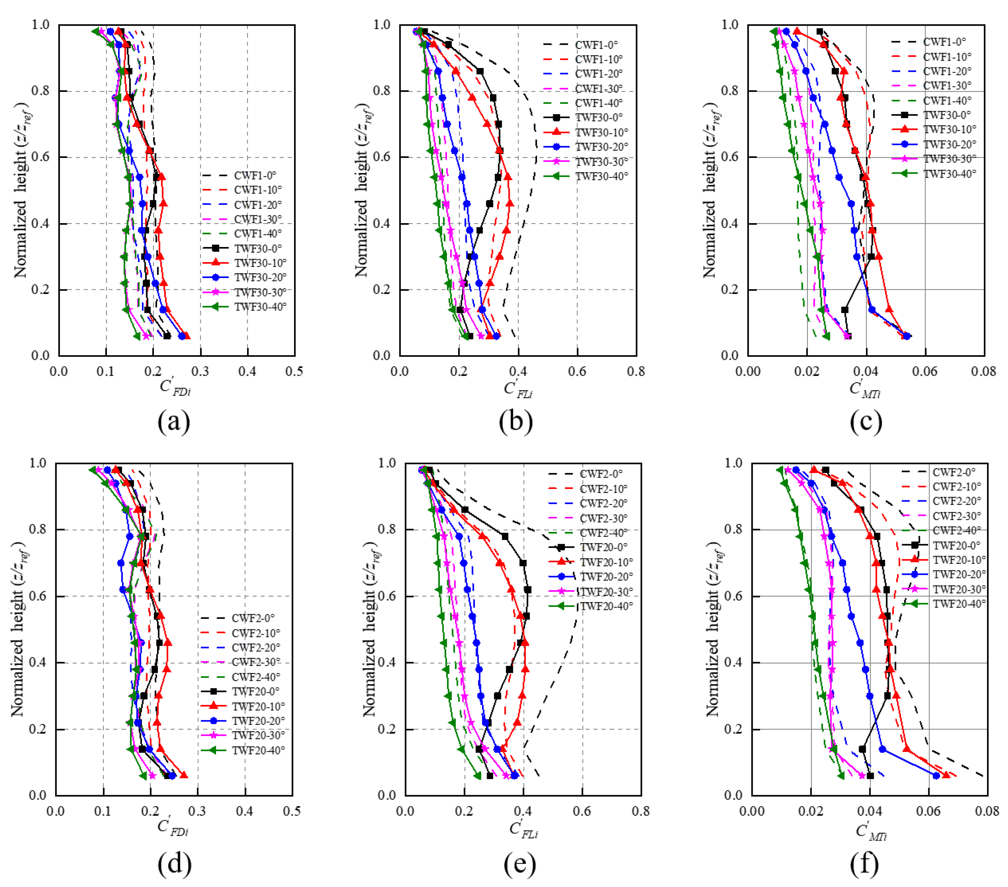
3.3.1. Mean and Fluctuating Local Wind Force Coefficients

Figure 13 plots the variations of local force coefficients ${\overline{C}}_{FDi}$, ${\overline{C}}_{FLi}$, and ${\overline{C}}_{MTi}$ (subscript $i$ denotes the $i$-th layer) with height in the cases of ${\theta }_{ref}$ ranging from 0° to 40° in CWFs and TWFs. As the wind field changes from CWF1 to TWF30 or from CWF2 to TWF20, the variations of ${\overline{C}}_{FDi}$ in different ${\theta }_{ref}$ cases generally follow the same varying trend with height, while the values of ${\overline{C}}_{FDi}$ become slightly lower, which suggests a generally lower mean drag force under the twisted wind effect. Meanwhile, the values of ${\overline{C}}_{FLi}$ at all layers deviate further from zero in the cases of ${\theta }_{ref}\ge$ 20°, which indicates higher mean lift forces. Noticeable differences between the ${\overline{C}}_{MTi}$ values in the TWFs and those in the CWFs are mostly found in the lower section of the building, e.g., $z/z_{ref}$ < 0.6, where the wind direction varies rapidly with height. Figure 14 illustrates the local drag, lift, and torsional moment coefficients at each layer, denoted by $C_{FDi}^{\prime }$ (the subscript $i$ denotes the $i$-th layer), $C_{FLi}^{\prime }$, and $C_{MTi}^{\prime }$, respectively. As shown in Figure 14a,d, the $C_{FDi}^{\prime }$ values in the CWFs are almost the same at all layers, regardless of the wind approach angle, whilst those in the TWFs gradually decrease with height. The $C_{FDi}^{\prime }$ values in the TWFs are generally enveloped by those in the CWFs, except for the cases of ${\theta }_{ref}$ = 10° and 20° at $z/z_{ref}$ < 0.6. Similarly, as presented in Figure 14b,e, the $C_{FLi}^{\prime }$ values in the TWFs are entirely enveloped by those in the CWFs. These observations suggest that the twisted wind effect results in a significant decrease in $C_{FLi}^{\prime }$ at all heights, which coincides with the findings in previous studies [26,27,28]. Regarding the torsional moments, the discrepancies between the $C_{MTi}^{\prime }$ values in the CWFs and those in the TWFs are mostly observed when ${\theta }_{ref}$ < 20°. Nevertheless, the varying range of $C_{MTi}^{\prime }$ with height was generally below 0.04, and therefore, such variation may be reasonably neglected from the perspective of wind-resistant designs of tall buildings.

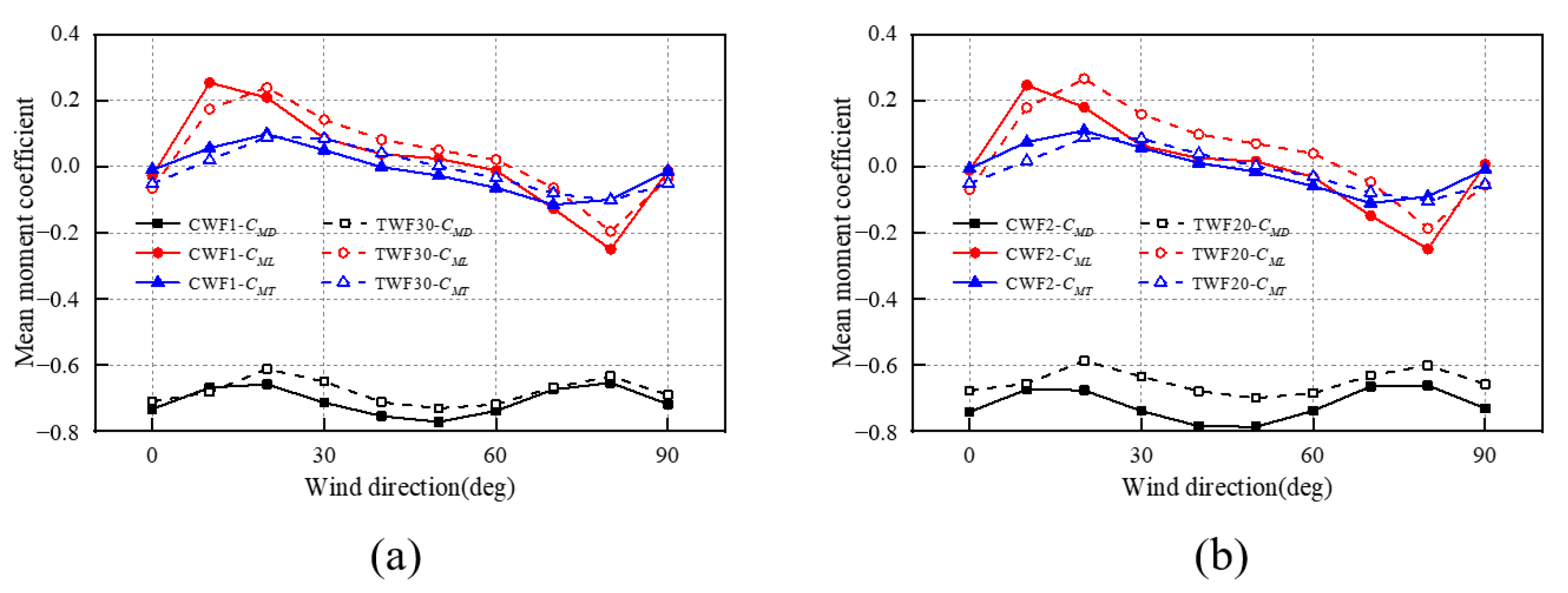
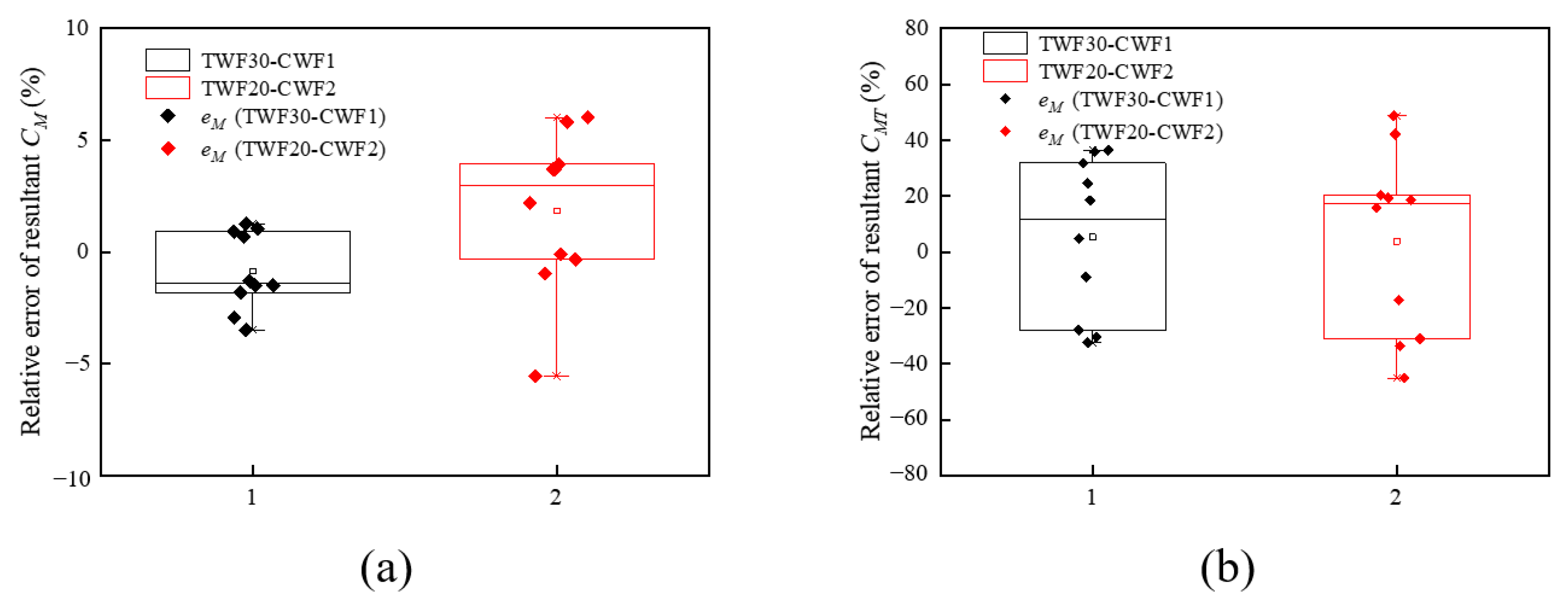
3.3.2. Mean Overturning Moment Coefficients

Figure 15 presents the variations of the mean overturning and torsional moment coefficients (i.e., , ${\overline{C}}_{ML}$, and ${\overline{C}}_{MT}$) with the wind approach direction ${\theta }_{ref}$ under both CWFs and TWFs. Due to the symmetry of the building, which is a square prism in shape, the variation of these moment coefficients with ${\theta }_{ref}$, as shown in the figure, are symmetric with respect to the case of ${\theta }_{ref}$ = 45°, implying an adequate accuracy of the wind tunnel test results presented in this study. As shown in Figure 15a, both the values and the varying trends of the moment coefficients with ${\theta }_{ref}$ in TWF30 are similar to those in CWF1. The maximum (absolute value) ${\overline{C}}_{MD}$, ${\overline{C}}_{ML}$, and ${\overline{C}}_{MT}$ in TWF30 (i.e., 0.73, 0.24, and 0.10, respectively) are slightly lower than those under CMF1 (0.77, 0.25, and 0.11, respectively). Comparing with the discrepancies between the moment coefficients in TWF30 and those in CWF1, as discussed above, the discrepancies observed from the TWF20 and the CWF2 cases appear to be slightly larger, as shown in Figure 15b. The maximum ${\overline{C}}_{MD}$ = 0.70 in TWF20 is noticeably lower than ${\overline{C}}_{MD}$ = 0.79 in CWF2, whilst the maximum ${\overline{C}}_{ML}$ = 0.27 in TWF20 is very close to ${\overline{C}}_{ML}$ = 0.25 in CWF2.

To further discuss the difference between the moment coefficients in CWFs and those in TWFs, Figure 16 presents the relative errors of those coefficients in the form of a boxplot. The relative errors of the overturning and torsional moments, denoted by $e_M$ and $e_{MT}$, respectively, are calculated as follows:

$$e_M=\frac{C_{M,TWF}-C_{M,CWF}}{C_{M,TWF}}$$

(19)

$$e_{MT}=\frac{\left|C_{MT,TWF}\right|-\left|C_{MT,CWF}\right|}{\max \left\{\left|C_{MT,CWF}\right|\right\}}$$

(20)

where $C_{M,TWF}$ (or $C_{MT-TWF}$) and $C_{M,CWF}$ (or $C_{MT-CWF}$) denote the values of $C_M$ (or $C_{MT}$) caused by TWF and CWF, respectively. It may be observed in Figure 16a that the $C_M$ values in TWF30 deviate from those in CWF1 by approximately −4% to 2%, while the $C_M$ values in TWF20 deviate from those in CWF2 from approximately −6% to 6%. Given the small magnitudes of the relative errors of the overturning moment coefficients, it appears that the wind tunnel test results of the overturning moments obtained in the CWFs are generally applicable to those in the TWFs. As presented in Figure 16b, the values of $e_{MT}$ in TWF30 range from approximately −30% to 40%, and those in TWF20 range from approximately −40% to 50%. Such high values of $e_{MT}$ suggest that the building torsional moment is considerably affected by the twisted wind effect, whereas it is also noteworthy that the torsional moment is usually insignificant for a high-rise building with a square sectional shape.

3.4. Characteristics of Correlation and Coherence of Local Wind Loads under Twisted Wind Effect

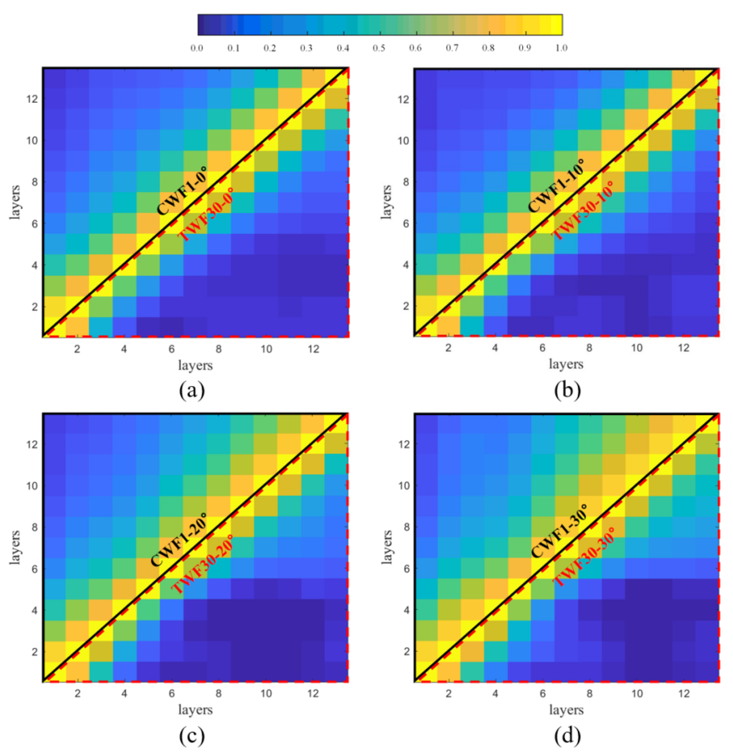
3.4.1. Correlation Coefficients

To investigate the spatial correlation of local wind loads at different heights of the building in the time domain, Figure 17 and Figure 18 plot the correlation coefficients (i.e., $Coh\left(z_i,z_j\right)$ expressed by Equation (14)) of the along- and across-wind loads, respectively, at different layers in TWF30 and CWF1. Figure 17 shows that, compared with the correlation coefficients of the along-wind load in CWF1-0° and CWF1-30°, those in TWF30-0° and TWF30-30° decrease more rapidly as the distance between the two layers increases. For instance, the correlation coefficients of the along-wind load in CWF1-0° are over 0.8 between one layer and its ±2 layers, whilst this is only true for ±1 layers in TWF30-0° at any ${\theta }_{ref}$. As the wind direction increases, the correlation coefficients of the along-wind load between the two upper layers (i.e., layer number $i$ ≥ 9) gradually grows, whilst that between the lower layers stays almost changed. On the other hand, the correlation coefficients of the across-wind load in TWF30-0° appear to be very similar to those in CWF1-0°, as shown in Figure 18a, whilst a noticeable difference in these coefficients is observed in Figure 18d, which compares the cases of TWF30-30° and CWF1-30°. As ${\theta }_{ref}$ reaches 30°, the correlation coefficients of the across-wind load between two separated different layers (i.e., $\left|i-j\right|$ ≥ 2) in TWF30 become less than 0.6, which is obviously lower than that in CWF1. Since the across-wind load of the building is caused by the vortex shedding generated at the leading edges, such a low correlation coefficient of the local across-wind load implies that the vortex shedding patterns in the TWFs are considerably different from those in the CWFs. As illustrated in Figure 19, the variations of the correlation coefficients of the along- and across-wind loads in CWF2-0° and TWF20-0° also demonstrate similar patterns to those discussed above.

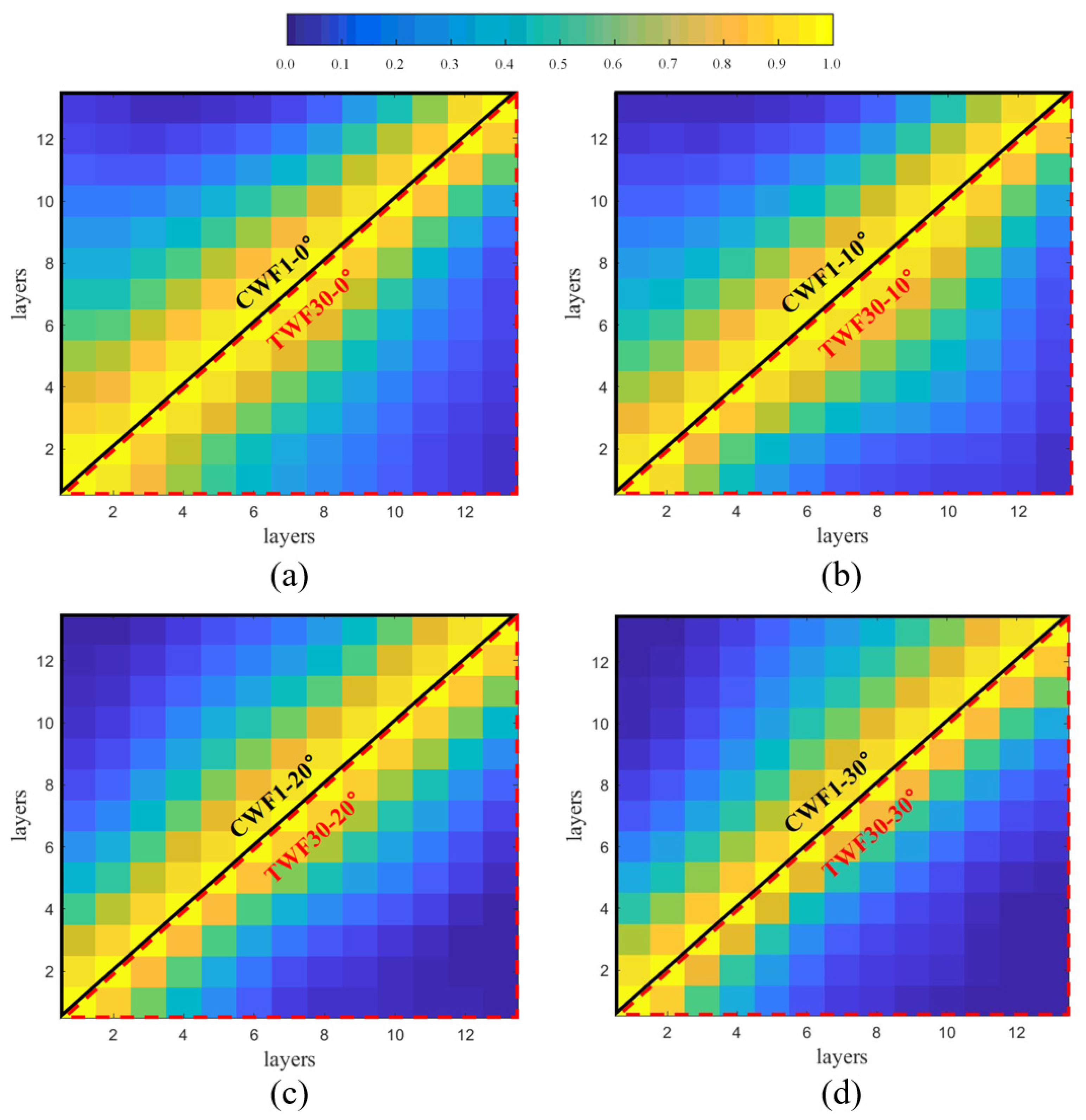
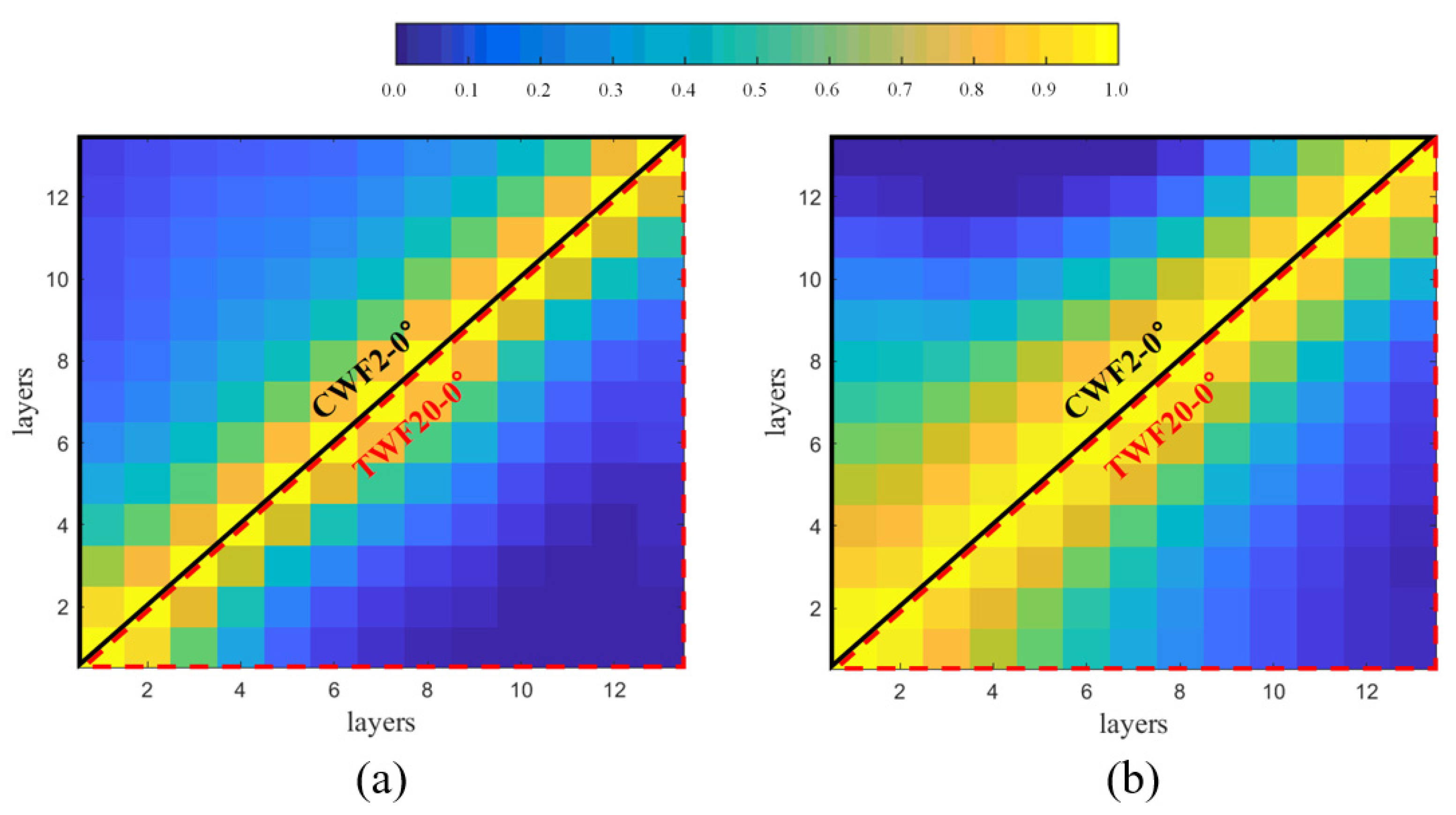
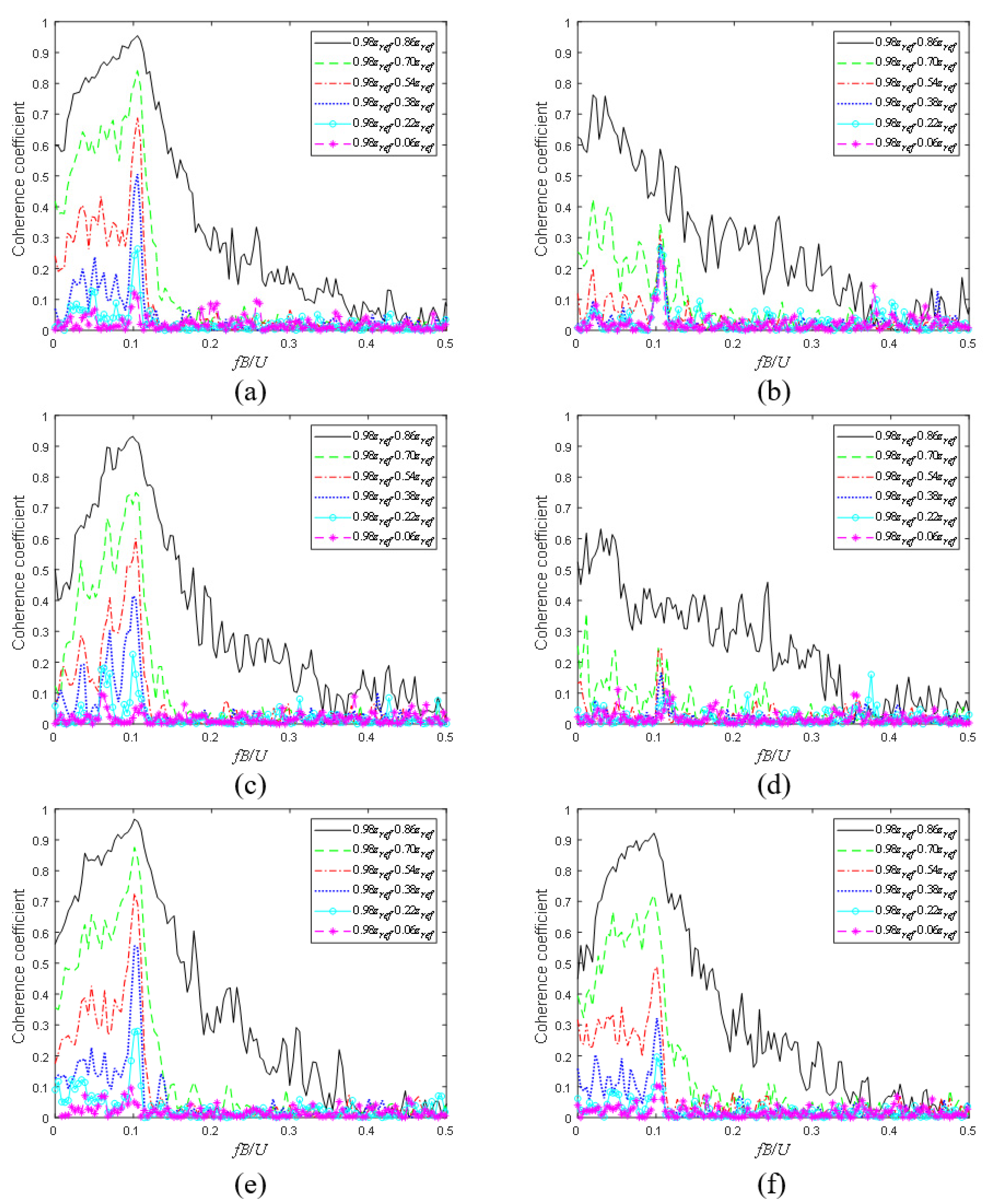
3.4.2. Characteristics of Coherence

Figure 20 illustrates the coherence coefficients (i.e., $Cor\left(z_i,z_j\right)$ expressed by Equation (15)) of the local across-wind load between the top layer ($z/z_{ref}$ = 0.98) and the six other selected layers ($z/z_{ref}$ = 0.86, 0.70, 0.54, 0.38, 0.22, 0.06) against the reduced frequency, which is expressed by

$$f_r=\frac{fB}{U}$$

(21)

where $f_r$ denotes the non-dimensional reduced frequency, $f$ denotes the frequency in Hz, $B$ denotes the characteristic length of the building that equals its breadth or depth, and $U$ denotes the mean wind speed. As expected, Figure 20 shows that the coherence coefficient is higher if the two layers are located more closely to one another. It is readily observed from the figure that the coherence coefficients of the different pairs of layers all peak at $f_r$ around 0.1, which essentially corresponds to the vortex shedding frequency of the building. At a frequency range of $f_r\le 0.05$, the coherence coefficients under TWFs (e.g., TWF30-0°, TWF30-30°, and TWF20-0°) are generally lower than those under CWFs (e.g., CWF1-0°, CWF1-30°, and CWF2-0°) by 0.1 to 0.2, indicating that the twisted wind effect diminishes the coherence between the local across-wind loads applied at different layers of a building.

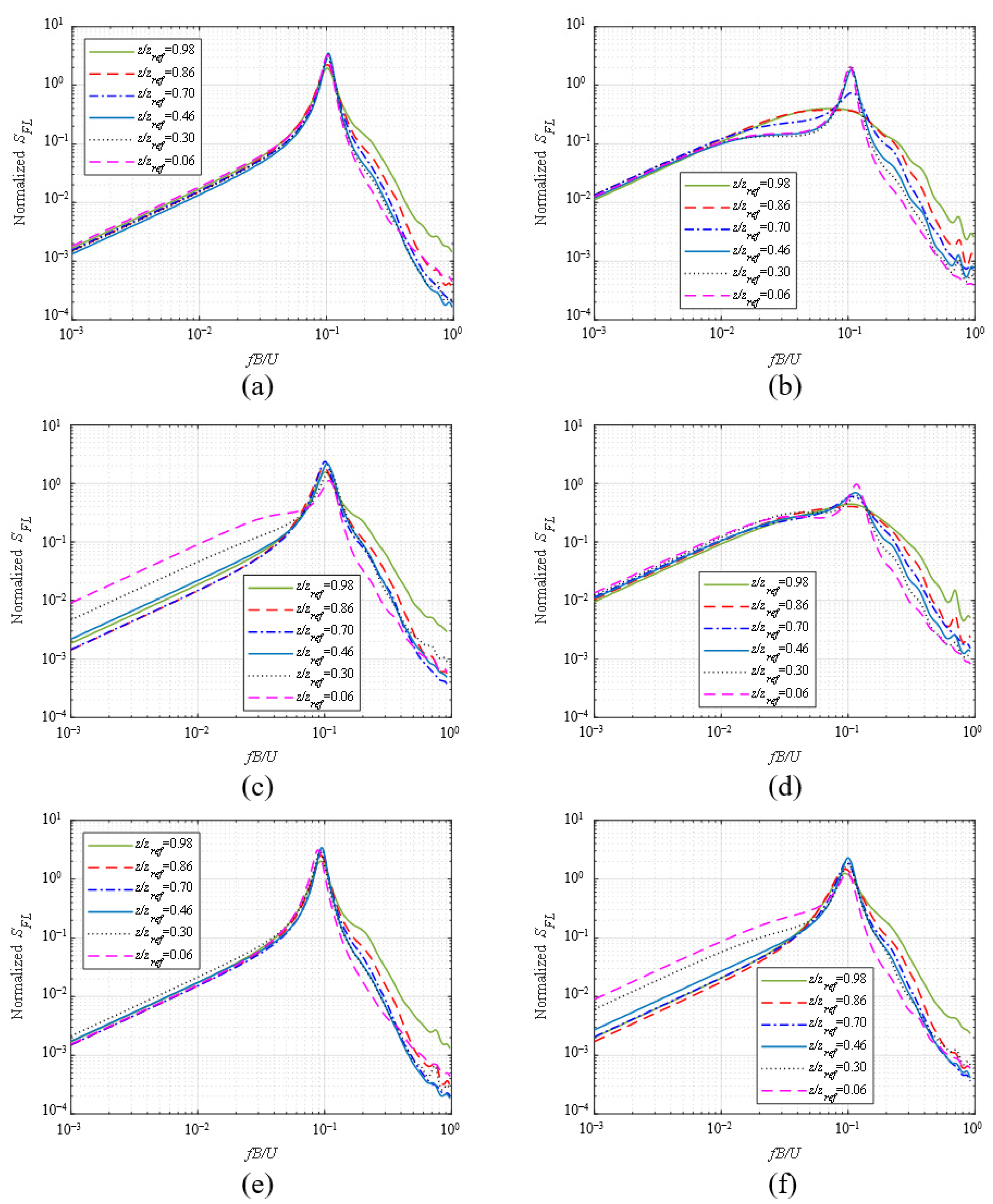
3.4.3. Power Spectra of Local Across-Wind Load

To investigate the local across-wind load in the frequency domain, Figure 21 illustrates the power spectral densities (PSDs) of local across-wind load. The spectral peaks, which correspond to the vortex shedding frequency, are observed at $f_r$ around 0.1 under both CWFs and TWFs. Notably, although the mean wind speed at layer $z/z_{ref}$ = 0.98 is the highest among all layers, the spectral peak corresponding to this layer is not the highest. This is because the flow toward this layer may pass around the building over the top instead of the side facades, resulting in less across-wind load on the building.

It is observed from Figure 21 that the vortex shedding frequency under TWFs gradually increases as the height $z/z_{ref}$ decreases, which is reasonable, because the wind approaches from an oblique direction at the lower part of the building, leading to a characteristic length which is larger than the building breadth, i.e., $B$ in Equation (18). Compared with the PSDs corresponding to layers $z/z_{ref}\le$ 0.30 in CWF1-0° and CWF2-0°, those in TWF30-0° and TWF20-0° demonstrate lower spectral peaks, and the PSDs within the frequency range below the vortex shedding frequency are noticeably higher. Such an observation indicates that the across-wind load at layers $z/z_{ref}\le$ 0.30 under the twisted wind effect is more evenly distributed over a wider frequency range (i.e., less concentrated at the vortex shedding frequency), and therefore, that the across-wind responses at these layers are mitigated to a certain extent. Similar observations are also obtained from the comparison between the PSDs under CWF1-30° and TWF30-30°. The spectral peaks corresponding to layers $z/z_{ref}\le$ 0.46 are diminished under the twisted wind effect, whilst the PSDs corresponding to these layers increase within the frequency range of 0.01 to 0.08, indicating the mitigation of the building across-wind response.

4. Concluding Remarks and Future Prospects

In this paper, a series of pressure model wind tunnel tests were conducted to investigate the wind pressure distributions and wind loads applied to a typical super-tall building under the twisted wind effect. The main findings and conclusions are as follows:

• The mean wind pressures on the building facades demonstrate asymmetric distribution under the twisted effect. With an oblique wind approach direction (e.g., ${\theta }_{ref}$ ≥ 30° under TWF30), one of the side facades may simultaneously be subjected to both positive and negative mean wind pressures in different parts. Compared with the application of CWF, both side facades are subjected to less suction force due to the twisted wind effect;
• Quantified by skewness and kurtosis, the wind pressures on the windward facade still follow the Gaussian distribution under the twisted wind effect, whilst those on the side and leeward facades demonstrate more prominent non-Gaussianess than is the case with a conventional wind field. The absolute values of the peak pressure coefficients under the twisted wind effect do not exceed those in the conventional wind field case, indicating that extreme wind pressures are mitigated under the twisted wind effect;
• Compared with CWF, the amplitudes of the along- and across-wind overturning moments only change slightly in TWF, suggesting that the wind tunnel test results obtained with CWFs are generally applicable to those with TWFs. Meanwhile, the torsional moment is significantly affected by the twisted wind effect, although the torsion is usually not a major concern for the wind-resistant design of tall buildings with square sectional shapes;
• Both the correlations and the coherences among local across-wind loads at various heights are diminished under the twisted wind effect, which is believed to be a result of the difference between the vortex shedding patterns in TWFs and those in CWFs. According to the power spectra of the local across-wind load at different heights, the across-wind responses of the lower section of a building are mitigated under the twisted wind effect.

Based on the above findings, this study highlights two points regarding the twisted wind effect that need to be considered for the improvement of building design. First, the estimates of extreme wind pressure on the windward facade need to be carefully examined, because the wind pressures in a TWF do not follow conventional Gaussian distribution. Second, the torsional moment in a TWF at a given wind approach angle noticeably differs from that in a CWF, and therefore, the design wind loads, particularly the local wind force, need to be estimated with caution.

While this paper focused on the twisted wind effect on a tall building that is square-prism in shape, the main findings are briefly summarized below for future research. First, the twisted wind effect on buildings with complex exterior geometries, especially those with common aerodynamic modifications, such as recessed corners and tapering, should be further investigated. Additionally, models to identify correlations between the parameters of the twisted wind effect (e.g., yaw angle) and the wind load on structures need to be proposed.

References

1. Ekman, V.W. On the influence of the Earth’s rotation on ocean currents. Ark. Mat. Astr. Fys. 1905, 2, 1–52. [Google Scholar]
2. Dyrbye, C.; Hansen, S.O. Wind Loads on Structures. Wiley: New York, NY, USA, 1997. [Google Scholar]
3. Mickle, R.E.; Cook, N.J.; Hoff, A.M.; Jensen, N.O.; Salmon, J.R.; Taylor, P.A.; Tetzlaff, G.; Teunissen, H.W. The Askervein Hill Project: Vertical profiles of wind and turbulence. Bound. Layer Meteorol. 1988, 43, 143–169. [Google Scholar] [CrossRef]
4. Cham, C.S.Y.; Kwok, K.C.S. Terrain characterization and design wind profiles for Hong Kong. Hong Kong Eng. Trans. 2011, 18, 2–9. [Google Scholar]
5. Tse, K.T.; Weerasuriya, A.U.; Kwok, K.C.S. Simulation of twisted wind flows in a boundary layer wind tunnel for pedestrian-level wind tunnel tests. J. Wind Eng. Ind. Aerodyn. 2016, 159, 99–109. [Google Scholar] [CrossRef]
6. Mendenhall, B.R. Statistical Study of Frictional Wind Veering in the Planetary Boundary Layer. Ph.D. Dissertation, Colorado State University, Fort Collins, CO, USA, 1967. [Google Scholar]
7. Tamura, Y.; Iwatani, Y.; Hibi, K.; Suda, K.; Nakamura, O.; Maruyama, T.; Ishibashi, R. Profiles of mean wind speeds and vertical turbulence intensities measured at seashore and two inland sites using Doppler sodars. J. Wind Eng. Ind. Aerodyn. 2007, 95, 411–427. [Google Scholar] [CrossRef]
8. Liu, Z.; Zheng, C.; Wu, Y.; Song, Y. Investigation on characteristics of thousand-meter height wind profiles at non-tropical cyclone prone areas based on field measurement. Build. Environ. 2018, 130, 62–73. [Google Scholar] [CrossRef]
9. He, Y.C.; Chan, P.W.; Li, Q.S. Observations of vertical wind profiles of tropical cy-clones at coastal areas. J. Wind Eng. Ind. Aerodyn. 2016, 152, 1–14. [Google Scholar] [CrossRef]
10. Shu, Z.R.; Li, Q.S.; He, Y.C.; Chan, P.W. Observational study of veering wind by Doppler wind profiler and surface weather station. J. Wind Eng. Ind. Aerodyn. 2018, 178, 18–25. [Google Scholar] [CrossRef]
11. Kim, Y.C.; Tamura, Y.; Tanaka, H.; Ohtake, K.; Bandi, E.K.; Yoshida, A. Wind-induced responses of super-tall buildings with various atypical building shapes. J. Wind Eng. Ind. Aerodyn. 2014, 133, 191–199. [Google Scholar] [CrossRef]
12. Kim, Y.C.; Bandi, E.K.; Yoshida, A.; Tamura, Y. Response characteristics of super-tall buildings—Effects of number of sides and helical angle. J. Wind Eng. Ind. Aerodyn. 2015, 145, 252–262. [Google Scholar] [CrossRef]
13. Flay, R.G.J. A twisted flow wind tunnel for testing yacht sails. J. Wind Eng. Ind. Aerodyn. 1996, 63, 171–182. [Google Scholar] [CrossRef]
14. Flay, R.G.J.; Vuletich, I.J. Development of a wind tunnel test facility for yacht aerodynamic studies. J. Wind Eng. Ind. Aerodyn. 1995, 58, 231–258. [Google Scholar] [CrossRef]
15. Flay, R.G.J.; Locke, N.J.; Mallinson, G.D. Model tests of twisted flow wind tunnel designs for testing yacht sails. J. Wind Eng. Ind. Aerodyn. 1996, 63, 155–169. [Google Scholar] [CrossRef]
16. Liu, Z.; Zheng, C.R.; Wu, Y.; Flay, R.G.J.; Zhang, K. Wind tunnel simulation of wind flows with the characteristics of thousand-meter high ABL. Build. Environ. 2019, 152, 74–86. [Google Scholar] [CrossRef]
17. Zhou, L.; Hu, G.; Tse, K.T.; He, X.H. Twisted-wind effect on the flow field of tall building. J. Wind Eng. Ind. Aerodyn. 2021, 218, 104778. [Google Scholar] [CrossRef]
18. Zhou, L.; Tse, K.T.; Hu, G. Experimental investigation on the aerodynamic characteristics of a tall building subjected to twisted wind. J. Wind Eng. Ind. Aerodyn. 2022, 224, 104976. [Google Scholar] [CrossRef]
19. Yuan, Y.J.; Yan, B.W.; Zhou, X.H.; Yang, Q.S.; Huang, G.Q.; He, Y.C.; Yan, J.H. RANS simulations of aerodynamic forces on a tall building under twisted winds considering horizontal homogeneity. J. Build. Eng. 2022, 54, 104628. [Google Scholar] [CrossRef]
20. Recommendations for Loads on Buildings. AIJ-2004. Architecture Institute of Japan: Tokyo, Japan, 2004.
21. Li, X.; Li, Q.S. Prediction models for modal parameters of super-tall buildings based on field measurements. J. Struct. Eng. 2020, 146, 06019004. [Google Scholar] [CrossRef]
22. Harris, R.I. An improved method for the prediction of extreme values of wind effects on simple buildings and structures. J. Wind Eng. Ind. Aerodyn. 1982, 9, 343–379. [Google Scholar] [CrossRef]
23. Cook, N.J.; Mayne, J.R. A refined working approach to the assessment of wind loads for equivalent static design. J. Wind Eng. Ind. Aerodyn. 1980, 6, 125–137. [Google Scholar] [CrossRef]
24. Cook, N.J. The Designer’s Guide to Wind Loading of Building Structures Part 2: Static Structures; Butterworths: London, UK, 1990. [Google Scholar]
25. Melbourne, W.H. Comparison of measurements on the CAARC standard tall building model in simulated model wind flows. J. Wind Eng. Ind. Aerodyn. 1980, 6, 73–88. [Google Scholar] [CrossRef]
26. Liu, Z.; Zheng, C.; Wu, Y.; Flay, R.G.J.; Zhang, K. Investigation on the effects of twisted wind flow on the wind loads on a square section megatall building. J. Wind Eng. Ind. Aerodyn. 2019, 191, 127–142. [Google Scholar] [CrossRef]
27. Zhang, X.L.; Weerasuriya, A.U.; Lu, B.; Tse, K.T.; Liu, C.H.; Tamura, Y. Pedestrian-level wind environment near a super-tall building with unconventional configurations in a regular urban area. Build. Simul. 2020, 13, 439–456. [Google Scholar] [CrossRef]
28. Mansour, W.; Tayeh, B.A.; Tam, L.-H. Finite element analysis of shear performance of UHPFRC-encased steel composite beams: Parametric study. Eng. Struct. 2022, 271, 114940. [Google Scholar] [CrossRef]
Figure 1. Guide vane system in wind tunnel: (a) schematics of twisted wind profile; (b) photo of experimental setup; (c) Elevation view; (d) top view.
Buildings 12 02260 g001
Figure 2. Wind profiles generated in wind tunnel tests: (a) Wind speed and turbulence intensity profiles of TWF30 and CWF1; (b) Wind speed and turbulence intensity profiles of TWF20 and CWF2; (c) Mean wind direction profiles of TWF30 and TWF20.
Buildings 12 02260 g002
Figure 3. Distribution of pressure taps on model facades (unit: mm).
Buildings 12 02260 g003
Figure 4. Photos of wind tunnel tests in the cases of (a) TWF30-0°; (b) TWF20-0°; (c) CWF1-0°; and (d) CWF2-0°.
Buildings 12 02260 g004
Figure 5. Definition of forces and moments applied to the building.
Buildings 12 02260 g005
Figure 6. Distributions of C ¯ p : (a) CWF1-0°; (b) TWF30-0°; (c) CWF2-0°; and (d) TWF20-0°.
Buildings 12 02260 g006
Figure 7. Distributions of C ¯ p in TWF30: (a) Windward facade; (b) Right facade; (c) Leeward facade; and (d) Left facade.
Buildings 12 02260 g007
Figure 8. Distributions of C ¯ p in TWF20: (a) Windward facade; (b) Right facade; (c) Leeward facade; and (d) Left facade.
Buildings 12 02260 g008
Figure 9. Skewness and Kurtosis of the pressure records at different layers: (a,b) CWF1-0°; (c,d) TWF30-0°; and (e,f) TWF30-30°.
Buildings 12 02260 g009
Figure 10. Skewness and Kurtosis of the pressure records at different layers: (a,b) CWF2-0°; and (c,d) TWF20-0°.
Buildings 12 02260 g010
Figure 11. Distributions of peak pressure coefficients: (a,b) CWF1-0°; (c,d) TWF30-0°; and (e,f) TWF30-30°.
Buildings 12 02260 g011
Figure 12. Distributions of peak pressure coefficients: (a,b) CWF2-0°; and (c,d) TWF20-0°.
Buildings 12 02260 g012
Figure 13. Variations of C ¯ F D i , C ¯ F L i , C ¯ M T i with height: (ac) in TWF30 and CWF1; and (df) in TWF20 and CWF2.
Buildings 12 02260 g013
Figure 14. Variations of C F D i , C F L i , C M T i with height: (ac) in TWF30 and CWF1; and (df) in TWF20 and CWF2.
Buildings 12 02260 g014
Figure 15. Variations of C ¯ M D , C ¯ M L , C ¯ M T with θ r e f : (a) TWF30 and CWF1; and (b) TWF20 and CWF2.
Buildings 12 02260 g015
Figure 16. Relative errors of (a) CM and (b) CMT between CWFs and TWFs.
Buildings 12 02260 g016
Figure 17. Correlation coefficients of along-wind load among different layers: (a) θ r e f = 0°; (b) θ r e f = 10°; (c) θ r e f = 20°; and (d) θ r e f = 30°.
Buildings 12 02260 g017
Figure 18. Correlation coefficients of across-wind load among different layers: (a) θ r e f = 0°; (b) θ r e f = 10°; (c) θ r e f = 20°; and (d) θ r e f = 30°.
Buildings 12 02260 g018
Figure 19. Correlation coefficients of (a) along-wind load and (b) across-wind load among different layers in the case of θ r e f = 0°.
Buildings 12 02260 g019
Figure 20. Coherence coefficients of across-wind load among different layers: (a) CWF1-0°; (b) CWF1-30°; (c) TWF30-0°; (d) TWF30-30°; (e) CWF2-0°; and (f) TWF20-0°.
Buildings 12 02260 g020
Figure 21. Power spectral densities of local across-wind load: (a) CWF1-0°; (b) CWF1-30°; (c) TWF30-0°; (d) TWF30-30°; (e) CWF2-0°; and (f) TWF20-0°.
Buildings 12 02260 g021