Abstract
It is often computationally expensive to monitor structural health using computer models. This time-consuming process can be relieved using surrogate models, which provide cheap-to-evaluate metamodels to replace the original expensive models. Because of their high accuracy, simplicity, and efficiency, Artificial Neural Networks (ANNs) have gained considerable attention in this area. This paper reviews the application of ANNs as surrogates for structural health monitoring in the literature. Moreover, the review contains fundamental information, detailed discussions, wide comparisons, and suggestions for future research. Surrogates in this literature review are divided into parametric and nonparametric models. In the past, nonparametric models dominated this field, but parametric models have gained popularity in the recent decade. A parametric surrogate is commonly supplied with metaheuristic algorithms, and can provide high levels of identification. Recurrent networks, instead of traditional ANNs, have also become increasingly popular for nonparametric surrogates.
1. Introduction
Damage to structures can arise from both artificial and natural causes, such as ageing and earthquakes, which result in thousands of deaths and billions of dollars of economic loss every year [1]. Hence, it is of crucial importance to constantly monitor structures and detect possible damage, and enhance their service life and safety. There are different categories for Structural Health Monitoring (SHM) based on the type of data, methodology, level of monitoring, etc. [2]. The most basic SHM method is visual inspection, which suffers from serious drawbacks in terms of accuracy, timing issues, interpretability of reports, and accessibility [3]. A number of Non-Destructive Testing (NDT) methods have been developed to address these shortcomings, such as impact echo, thermography, ultrasound electrical resistivity, and Ground-Penetrating Radar (GPR) [4]. However, most of these methods are local, which means that the defect’s location must be known beforehand, because a complete scan of large structures can be extremely time consuming. On the other hand, there exist SHM methods at the global level that assume structural damage affects the dynamic behavior of the structure, and can be identified through processing its response. Figure 1 demonstrates the main goals, testing methods, data analysis techniques, and inputs and outputs of common vibration-based SHM methods.
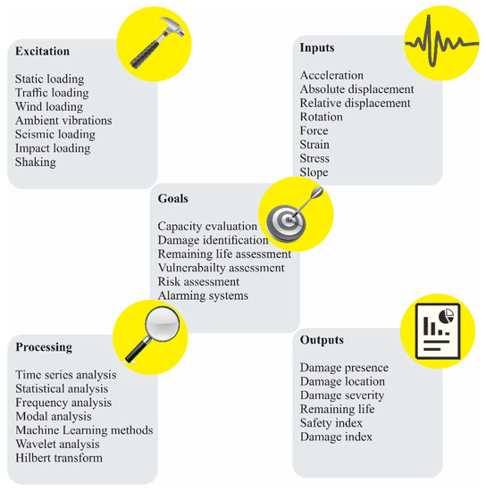
Figure 1.
Five main components of vibration-based SHM.
As a major classification, the methods can be categorized either as model-based or non-model-based. Model-based methods require a numerical model of the structure, e.g., the Finite Element (FE) model, while non-model-based methods need only the recorded data from structures. The non-model-based methods commonly provide level 1 (i.e., determination of damage presence) or level 2 (i.e., level 1 plus damage localization) monitoring, while model-based methods can obtain level 3 (i.e., level 2 plus damage quantification) or level 4 (i.e., level 3 plus remaining life prediction) identifications [5]. Therefore, among various damage identification methods, model-based techniques have drawn considerable attention in recent years [6].
The model-based methods usually involve repeated evaluation of the structural model, which is a time-consuming and computationally prohibitive task. On the other hand, in SHM applications, it is necessary to identify damages online or within a reasonably short time. This issue has motivated researchers to replace them with cheap-to-evaluate data-driven models. There are several terms used in the literature to describe these computationally inexpensive models, including surrogates, emulators, and metamodels. Surrogates have widespread applications in other scientific fields besides SHM, such as uncertainty quantification [7], sensitivity analyses [8], and optimization [9], to avoid long model runtimes. A wide variety of surrogate models, such as Least Squares Approximation (LSA), Response Surface Models (RSMs), Support Vector Machines (SVMs), kriging, and Artificial Neural Networks (ANNs), have been developed over the years. They are commonly constructed through a data-driven procedure relating a set of dependent variables (inputs) to one or more independent variables (outputs).
It is believed that the first publication of ANN in civil engineering dates back to 1989, when a simple ANN was applied to design a steel beam [10]. In recent years, the rise of big data, adoption of high-performance processors, and enormous potential of ANNs—as universal approximators—have led to significant growth in their application to civil engineering, in general, and SHM, in particular. Although several review papers have been published on the application of Machine Learning (ML) methods and ANNs in SHM [11,12,13,14,15], according to our best knowledge, few of them have provided discussions about the role of ANNs as emulators in SHM.
Toh and Park [13] summarized research studies that have applied machine learning algorithms for fault monitoring. They divided publications into several categories in terms of types of vibrations, including power-source-induced, rotational, external, and ambient vibrations. Their main focus was on deep learning algorithms and mechanical systems, such as gearboxes and rotating machines. Akinosho, et al. [14] reviewed the application of deep learning in a broad range of challenges in the construction industry: SHM, workforce assessment, construction safety, and energy demand prediction. This paper has reviewed only two papers applying vibration data for SHM. Xie, et al. [11] conducted a comprehensive review of the earthquake engineering publications covering seismic hazard analysis, damage identification, fragility assessment, and structural control. They adopted a hierarchical methodology based on the employed algorithm, topic area, resource of data, and analysis scale. Since their search was constrained by both “machine learning” and “earthquake engineering” keywords, their review lacks some of the studies that use input excitations apart from seismic loading, and covers few studies applying surrogate ANN. A systematic review of deploying ML algorithms in civil SHM was presented by Flah, et al. [12]. They focused mostly on the studies deploying ANNs and Support Vector Machines (SVMs) that have been conducted in the recent decade. Although vision-based publications have been covered appropriately in their review, many of the research studies on vibration-based surrogates have been neglected. On the other hand, Avci, et al. [15] expended considerable effort to present a detailed review of vibration-based approaches. In this review, ML-based SHM was comprehensively analyzed; however, the focus was on parametric ANNs (PNNs) via 1D CNNs rather than emulator ANNs (ENNs), which is the main focus of the current paper. In addition, even though many details and results have been presented in their review, they have not provided a unifying perspective on applied paradigms.
In this literature review, we intend to conduct a detailed survey of the papers applying ANNs as surrogates for the SHM of civil structures. In this regard, combinations of different keywords, including “surrogate”, “emulator”, “metamodel”, “structural health”, “damage detection”, “damage identification”, “model updating”, “wave propagation”, and “neural networks”, were adopted to explore the literature in the Google Scholar search engine. Ultimately, irrelevant articles to the scope of the review paper were excluded, and the remaining journal papers, conference articles, and book chapters were collected. They were classified as parametric or nonparametric models based on the developed surrogates. In this literature review, we extract and discuss the main ideas as well as interesting details, such as inputs, outputs, and hyperparameters.
2. Artificial Neural Networks
ANNs are inspired by the way information is processed and distributed in biological neurons, and derive their name from this process [16]. Theoretically, ANN is a parametric representation of a nonlinear function parameterized by , which maps inputs to produce outputs . Since the neural networks apply differentiable functions, a gradient-based optimization algorithm can be utilized to minimize a scalar loss function related to how far the network output is from the desired output and determine optimum parameters. The backpropagation algorithm is widely used to compute gradients for neural networks [17]. The process of optimization is known as neural network training, which applies the backpropagation algorithm for the iterative improvement of parameters. Mathematically, the training is defined by the following formulation:
where is the dataset of available input–output pairs.
ANNs are typically constructed to pass the input through a series of layers. Every layer in a feedforward network applies an affine transformation by calculating the weighted sum and adding a bias , followed by a nonlinear elementwise activation function :
Some of the most common activation functions—also called transfer functions—are presented in Figure 2.
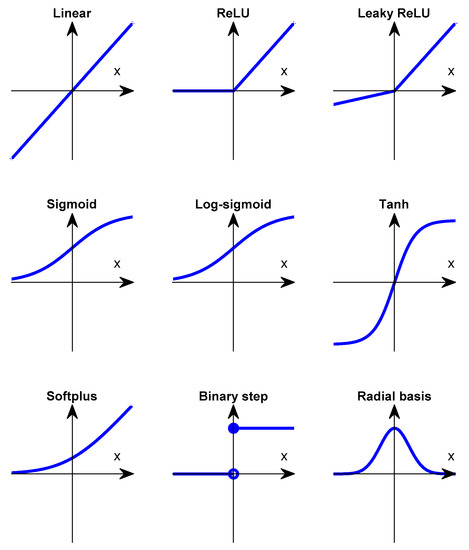
Figure 2.
Common activation functions.
In principle, any function can be approximated by a sufficiently large, single-layer neural network [18]; however, it is possible to learn complex features more efficiently by adding extra layers to the model [19]. A network with many layers is usually called a deep network, and its training process is known as deep learning.
2.1. Types of Neural Networks
Several types of neural networks with different sets of parameters, operations, and architectures have been developed and implemented for various applications. In the following, we briefly introduce the most common neural networks used in the SHM literature.
2.1.1. Multi-Layer Perceptron (MLP) Neural Networks
A Multi-Layer Perceptron (MLP) is the basic fully connected class of feedforward ANNs, which often refer to any feedforward ANN. As shown in Figure 3, they usually consist of three layers (an input layer, a hidden layer, and an output layer), but the number of layers can be increased.
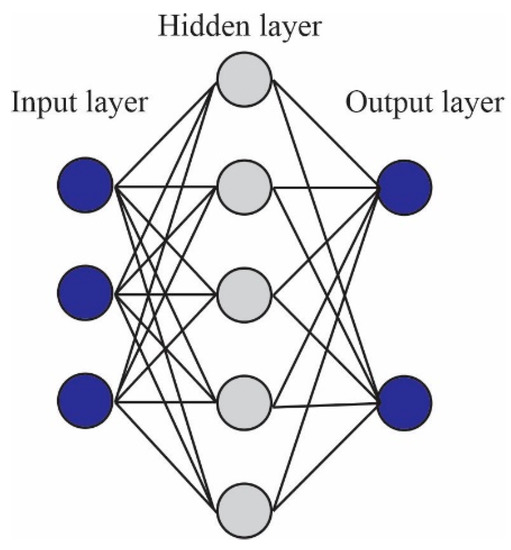
Figure 3.
An example of an MLP network with one hidden layer.
2.1.2. Radial Basis Function Networks (RBFNs)
Radial Basis Function Networks (RBFNs) use radial basis activation functions (RBFs) [20], as shown in Figure 2. The output of an RBFN is a linear combination of the radial basis of the inputs and neuron parameters. They usually have three layers: an input layer, a hidden layer with a nonlinear RBF activation function, and a linear output layer. RBF’s value depends on the distance between the input and a fixed point, which is called the center. There are different types of radial functions, all of which can be presented in the form of a radial kernel, as follows:
where is the input, denotes the center point, and represents the Euclidian distance.
2.1.3. Cascade Feedforward Neural Network (CFNN)
In Cascade Feedforward Neural Networks (CFNNs), the input layer is connected to all hidden layers as well as the output layer [21]. It starts with one layer and gradually adds new layers and trains the network until achieving the best performance. Unlike the basic MLP networks, a CFNN is capable of including both linear and nonlinear relationships between inputs and outputs in a multi-layered architecture. Figure 4 shows a typical CFNN structure.
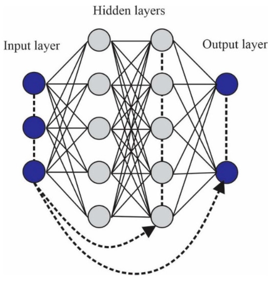
Figure 4.
The typical architecture of a CFNN.
2.1.4. Group Method of Data Handling (GMDH) Network
Group Method of Data Handling (GMDH) considers various partial models whose coefficients are estimated through the least square method [22]. The coefficients as well as a predefined selection criterion determine which partial models should be kept and which ones need to be removed, as can be seen in Figure 5. It starts with one model and gradually increases the complexity by including new partial models until reaching a preselected optimal complexity. By so doing, the GMDH neural network self-selects the optimum architecture, including the activation functions and the number of hidden layers, which is called model self-organization.
Figure 5.
The architecture of a GMDH network.
2.1.5. Extreme Learning Machine (ELM)
Extreme Learning Machines (ELMs) have been proposed to train single-hidden-layer networks, as illustrated in Figure 3 [23]. However, in contrast to traditional learning algorithms, ELMs have been originally designed to maximize generalized performance by minimizing both training errors and output weight norms, and do not need to be tuned iteratively. The output function of an ELM is defined as Equation (4):
where l represents the number of hidden neurons, h(x) denotes the activation function, N is the number of training samples, β denotes the weight vector between the hidden and output layers, and x is the input vector mapped into the ELM feature space. The hidden layer need not be tuned, and its parameters can be fixed randomly. The output weights are then calculated using the least square method, minimizing the approximation error:
where H is called the hidden layer output matrix, T is the vector of labels of the training dataset, and ‖•‖ denotes the Frobenius norm. The solution to the linear minimization problem is:
A Moore–Penrose-generalized inverse of matrix H is adopted to calculate . Hence, instead of an iterative backpropagation algorithm, the training is performed rapidly, requiring only one step for calculations.
2.1.6. Bayesian Neural Networks (BNNs)
In Bayesian Neural Networks (BNNs), the model weights take on a probability distribution rather than a single optimal value [24]. This allows them to generalize effectively, and makes them good candidates for probabilistic applications, such as uncertainty quantification or probabilistic damage identification. In order to update the network parameters and calculate the posterior distributions, the marginalization process based on Bayes’ rule is performed. Figure 6 presents a schematic of a BNN.
Figure 6.
A schematic of a BNN.
2.1.7. Recurrent Neural Network (RNN)
A Recurrent Neural Network (RNN) can save the outputs of a particular layer and feed them back to the input to predict the output of the next sample [17]. Such feedback loops make them capable of learning sequential data, each sample of which is dependent on previous ones. Figure 7 illustrates a simple RNN unit, which can be unfolded over time in the form of one to many, many to one, and many to many input–output architectures.
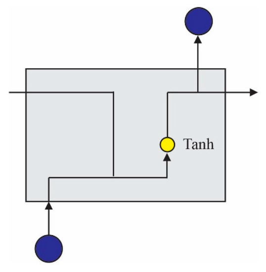
Figure 7.
Illustration of an RNN cell.
One of the special types of RNN is called a Long Short-Term Memory (LSTM) network, which usually outperforms the standard RNN [25]. They can learn both long-term and short-term dependencies in data. LSTMs have four main components—input gate, output gate, forget gate, and cell state—incorporated into their architecture, as shown in Figure 8.
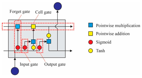
Figure 8.
Illustration of an LSTM cell.
2.1.8. Physics-Informed Neural Networks (PINNs)
In Physics-Informed Neural Networks (PINNs) the governing rules of the data, usually described by Partial Differential Equations (PDEs), are embedded in the loss function [26]. For example, the motion equations can be implemented in the response prediction of a dynamic system. By so doing, they overcome the data scarcity issue as well as the inability of standard ANNs in extrapolation. As can be seen in Figure 9, the derivatives of differential equations are calculated through automatic differentiation, upon which the PDE, Boundary Condition (BC), and Initial Condition (IC) residuals are calculated and incorporated into the total loss.
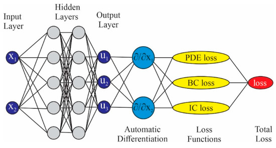
Figure 9.
A schematic of a PINN.
3. Artificial-Neural-Network-Based Surrogate Models
A review of the research papers that have applied ANNs as surrogate models for SHM of civil structures is presented in this section. For a clear comprehension, the studies have been classified into nonparametric and parametric surrogates. Generally, parametric surrogates are employed for inverse-model-updating-based damage identification, where damage parameters (such as degradation in modulus of elasticity or cross-sectional loss) are inputs and desired features are outputs. Nonparametric metamodels, on the other hand, do not use damage parameters, and instead apply measurements such as loadings, accelerations, and displacements, as inputs.
3.1. Nonparametric Surrogate Models for SHM
By considering structures as dynamical systems, neural network metamodels are capable of learning and forecasting the mapping between inputs and outputs of the systems. In early SHM paradigms, it was common to apply such metamodels, trained in the healthy state of the structure, in order to predict the responses of the structure at certain points, and compare them with the corresponding measurements in the real structure. The overall procedure of structural damage identification using these emulators is shown in Figure 10. As can be seen, there are four main steps in this process. The first step is to construct and train an Emulator Neural Network (ENN) using the simulated dynamic responses of the object structure under a set of ground excitations. In the second step, when the structure becomes damaged, the dynamic response of the structure forecasted with ENN would not match the real measurement under excitations. To compare the responses in the mentioned states and quantify the deviations, an evaluation index is used. The third step involves building and training a Parametric Evaluation Neural Network (PENN) to map the evaluation index into structural parameters, such as stiffness. Finally, the PENN forecasts the parameters to identify the damage in the fourth step. To detect the damage, inputs and outputs should have a clear physical meaning. A list of inputs and outputs used in different studies can be found in Table 1.
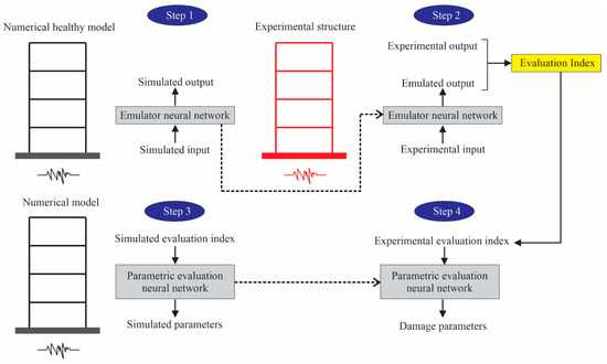
Figure 10.
The overall procedure of the application of nonparametric emulators for SHM.

Table 1.
Inputs and outputs of nonparametric surrogate models.
In 1997, Wong, et al. [27] developed an ANN for emulating the inter-story drifts in a two-story steel frame building. Then, a comparison module was designed to identify damage severity according to the deviation between the measured and emulated responses. It was shown that damage extent cannot be reliably determined from the response of a single ANN, and it is necessary to train specialized networks for varying states of damage, whose predicted responses can be utilized for damage classification.
Huang, et al. [29] proposed a method for extracting the modal parameters through the weight matrices of the ANN-based metamodel. The ANN was trained to predict the acceleration response of a five-story shear frame using input seismic base excitations. Comparing the model parameters extracted from the metamodel with Trifunac’s index [58], they detected the presence of damage in the frame. The index is given in Equation (7):
where = mode shape array of healthy structure corresponding to th degree of freedom, = mode shape array of healthy structure corresponding to the th degree of freedom (DOF), and is calculated by minimizing the nominator.
Xu, et al. [30] developed a localized emulator neural network that was able to predict the response of a substructure of a healthy frame. Based on the difference between the predicted and recorded responses, they could determine the health status of the structure. To this end, another neural network was trained to identify damage by predicting the stiffness of each story in the substructure. In this research, the Relative Root Mean Square () vector was used to evaluate the condition of the damaged structure, which is presented in Equation (8):
where = the number of sampling data, = the output of the metamodel corresponding to the th DOF at step , and = the measured response corresponding to the th DOF step .
In a similar study, Xu [37] indicated that Root Mean Square Prediction Difference (RMSPD) can be also employed for the evaluation of the substructure. This index is formulated in Equation (9):
where = the number of sampling data, = the output of the metamodel corresponding to the th DOF at step , and = the measured response corresponding to the th DOF at step .
Faravelli and Casciati [33] applied ANN and RSM for emulating the vertical displacement of a three-span bridge and accelerations of a three-story steel frame in a healthy state. They statistically compared the Sum of Squares Error (SSE) values, defined in Equation (10), between the damaged and healthy states through an F-test to ensure the presence of damage:
where = the number of sampling data, = the output of the metamodel corresponding to the th DOF at step , and = the measured response corresponding to the th DOF at step .
The damage can be localized by comparing the responses of measurements in every section of the structure.
Jiang, et al. [50] trained a Fuzzy Wavelet Neural Network (WNN) with a backtracking inexact linear search scheme, and applied it to the response prediction of two high-rise irregular building structures with geometric nonlinearities. They used wavelets to denoise the training input signal, and observed that the preprocessed data substantially improved the prediction accuracy. The error in all test evaluations was less than . Jiang and Adeli [40] applied the Fuzzy WNN network for predicting the dynamic response of a 38-story concrete test model. Then, they developed a new damage evaluation index, called a pseudospectrum, to perform damage detection. Compared with the RRMS index, they indicated that the new method is robust against noise and provides effective distinguishability for different damage severities. Mitchell, et al. [48] proposed a Wavelet-based Adaptive Neuro-Fuzzy Inference System (WANFIS) to predict the acceleration response of a nonlinear structure with an MR damper under an artificial seismic signal. The system applies the backpropagation algorithm to determine the fuzzy inference system’s membership functions. The system was tested on real earthquakes, and it was indicated that it requires a significantly shorter time than the Adaptive Neuro-Fuzzy Inference System (ANFIS) model, while providing higher accuracy. Khalid, et al. [49] applied an RNN to predict the output force of a damper of a semi-active controlled structure based on a supply voltage as well as input displacement and acceleration. Under different excitations with sinusoidal displacements, the model predicted the forces with less than maximum error.
Xu, et al. [32] presented an approach for detecting the presence of damage in a suspension bridge. In this study, they developed two separate networks for predicting the velocity in transversal and vertical directions on the deck of the bridge. Then, the RRMS was applied to indicate whether damage had occurred or not. In another research study, Xu, et al. [36] developed a similar framework for the identification of damage in a five-story shear building. Following these studies, Xu and Du [38] proposed a substructural acceleration-based emulator neural network for predicting the acceleration measurements of a substructure, with the linearly normalized acceleration measurements at the boundary nodes at three previous timesteps. A substructural PENN was developed to identify the stiffness and damping coefficients based on the RMSPD vector.
Xu, et al. [39] presented a three-step strategy to identify stiffness and damping parameters of a truss structure with induced strains by vibrations, which can be measured with FBG strain sensors. They applied an emulator neural network for predicting the structural macro-strain response of all members through feeding the strain responses at two past timesteps. In another work, Xu [45] made the method flexible in terms of incompleteness in the vibration strain. In this regard, the emulator network was trained with the measurements of a few members of the truss structure.
Inspired by the research conducted by Xu and his colleagues, Mita and Qian [41] proposed a neural network for emulating the structural response of a five-story shear frame. To train the network, they used acceleration measurements of different nodes at previous timesteps, with large delays, and the current timestep, as the inputs and output, respectively. A modified Relative Root Mean Square () error between the real dynamic response and the output of the neural network was applied as the damage index. Qian and Mita [44] optimized the time delay to find the most sensitive signals, and used various ground excitations to show the generality of their approach. The overall procedure and the emulator of this study were similar to their previous work [41]. The evaluation criterion of both studies is provided in Equation (11):
where = the number of sampling data, = the output of the metamodel corresponding to the DOF of at step , and = the measured response corresponding to the DOF of at step .
Wang, et al. [42] proposed a three-step framework to find the damage locations and severities in the Bill Emerson cable-stayed Bridge. In the first step, they developed an emulator network to predict the response of the bridge in the healthy state. In the second step, they trained a network relating the stiffness reduction in the bridge to the difference between the measured response and the response predicted in the first step. The third step was to identify the damage. Wang and Chen [43] trained two ANNs for damage identification in a highway bridge structure. The first ANN (ENN) was responsible for emulating the dynamic response of the bridge. The second ANN (PENN) was trained to forecast the damage extent given the difference between the measured and predicted dynamic responses. To evaluate the structures’ response, both studies used a Weighted Root Mean Square (WRMS) evaluation index, as presented in Equation (12):
where , = the number of sampling data, = the output of the metamodel corresponding to the DOF of at step , and = the measured response corresponding to the DOF of at step .
Wu, et al. [31] developed a decentralized identification method including two steps. First, they trained neural networks to forecast restoring forces of substructures of an intact multi-degrees-of-freedom (MDOF) system. Second, another network relating the RRMS evaluation index to the stiffness of the substructures was established to quantify the stiffness degradation in the substructure. Similarly, Choo, et al. [46] proposed a two-stage framework for the identification of damage presence, extent, and location in a three-span steel bridge. In the first stage, an ENN was trained to emulate the acceleration response at the top of the pier and superstructure in the healthy state, and in the second stage, another network was employed to output the actual restoring force of both intact and damaged states. Comparing the restoring force of the two states, one can obtain the time history of stiffness and damage. Xu, et al. [47] developed a two-stage method for damage identification in a frame structure with joint connection loosening. They trained an ENN for outputting displacement response and another network, fed with the RMSPDV, for forecasting the inter-story stiffness of floors.
The mentioned methodology was abandoned for a while, but following the huge development of neural networks, new studies began exploring the first step of the mentioned methodology (developing ENNs), after almost eight years. In 2017, Jiang, et al. [50] developed an advanced framework for determining the dimension of input and hidden neurons as well as dividing the input data into fuzzy clusters. To this end, the false nearest neighbor approach and Bayesian information criterion were employed. They applied the method to predict the response of two- and four-story steel frames, and observed that the sensed data could be predicted with over confidence.
Perez-Ramirez, et al. [51] proposed a three-step methodology for the nonparametric identification of large civil structures under seismic and ambient vibrations. They applied Empirical Mode Decomposition (EMD) to denoise the measured signals, and utilized the Mutual Information (MI) index to find the optimal number of hidden neurons in a NARX-NN emulator. Finally, a Bayesian algorithm was employed to train the network. They examined the performance of the method using a scaled model of a 38-story building as well as a five-story steel frame, and observed that the method can reduce the absolute error up to 80% and 25% compared with past methods (e.g., Jiang and Adeli [40]) and the non-optimal version, respectively. Vega and Todd [52] applied a BNN using variational inference to learn from a miter-gate-based high-fidelity FE model. The upstream and downstream hydrostatic pressures as well as temperature distributions were fed to the network to predict the gap length between the lock wall and the quoin block of the gate. The gap indicates a loss of bearing contact and change in the load path, which can lead to operational and structural failure, and therefore, can be considered as a direct index of damage. Xue, et al. [55] applied a CNN for predicting the time history response of a transmission tower excited with complex wind loading. As the input of the network, they converted the time and spatial wind speed into a single-channel image, and top displacement of the transmission tower was set as the output. Investigating the performance of different architectures and hyperparameters, they found that the window size and the scale of training data considerably influenced the forecasting error and computational time.
Zhang, et al. [53] introduced two physics-informed multi-LSTM network architectures for the metamodeling of nonlinear structural systems with scarce ground motion data. The first architecture interconnects two deep LSTM networks with a tensor differentiator, and was guided by motion equations and state dependency constraints. In the second architecture, there were three deep LSTM networks as well as a tensor differentiator, and the rate-dependent hysteretic behavior (Bouc–Wen model) was also encoded to emulate a nonlinear hysteresis structure. The comparisons showed that both metamodels can recognize the hidden patterns in data and provide robust results. Li, et al. [56] compared the performance of a data-driven LSTM network with the FE method in modeling bridge aerodynamics. They showed that the LSTM model outperforms the FEM, mainly due to the limitations of the Reynolds number effect and the Rayleigh damping hypothesis. Tan, et al. [57] presented a framework for predicting the mechanical behavior of an underwater shield tunnel. They applied an autoencoder to extract high-level features at different spatial positions, and an RNN to recognize the temporal correlations. The spatiotemporal information was combined with dynamic loading to predict the strain during the next 12 h by a fully connected ANN. They showed that the model, so-called ATENet, reaches % accuracy, and can be used in real-time performance predictions of underwater tunnels.
There has been considerable study of elastic wave propagation in nondestructive testing; however, most research studies rely on simple specimens, such as plates [28,59] or strips [60]. This is mainly because the behavior of the elastic wave is difficult to predict in structures with complex geometries. Elastic waves propagate in different directions until they encounter boundaries or defects in the medium, and then they reflect with new parameters. The anomalies and defects can be detected by monitoring the propagation of waves. Researchers have mostly applied ANNs for predicting or classifying damages [61,62,63,64,65,66,67,68,69] from the recorded data rather than surrogate modeling of structural systems. Additionally, in the literature, there is a lack of examples considering the application of this method in civil SHM. In other words, most studies have considered mechanical structures, such as aluminum plates [70], fabric composite panels [71,72], functionally graded material plates and cylinders [68,73,74], and flange connections [75,76,77]. Nonetheless, for the sake of completeness, we review studies that applied ANNs as surrogates for wave propagation and damage identification. We hope that with the advent of new paradigms, such as PINNs, this field will attract the attention of engineers and researchers in the near future.
Chandrashekhara, et al. [28] proposed an ANN surrogate for determining the contact force of laminated plates under low-velocity impact. Using higher-order shear-deformation-theory-based finite element simulations, they extracted contact forces and strain histories at three locations. Using these data, they trained ANNs that estimate the contact forces with the strain measurements given as inputs. They indicated that the developed model can be applied to online SHM systems.
Kim, et al. [34] developed a surrogate for predicting the stress intensity factor in a steel plate with ring-down counts, rise time, energy, duration, and peak amplitude of acoustic emission (AE). Fatigue crack parameters, such as crack length and geometry, can be related to the stress intensity factor. According to the results, the metric was between and for different specimens, indicating that traditional ANNs are not always successful in predicting such variables.
Recently, Shukla, et al. [54] utilized PINNs to characterize surface cracks in an aluminum plate subjected to ultrasonic acoustic waves with a frequency of MHz. The data were acquired by a laser vibrometry technique and included in the second-order PDE that governed the acoustic wave propagation:
where is the displacement field, subscript stands for the partial differentiation with regard to time, and denotes the sound speed. The loss function of the PINN was formulated as follows:
where represents the recorded data, corresponds to the governing PDE (Equation (13)), and represents a penalty factor.
To identify cracks, was approximated with given by experimental data. The presence of a crack manifested itself with a local change in the wave speed, due to near-field scattering of the energy as well as inelastic attenuation. They evaluated the network on four sets of data with different angles of the acquired wavefield, and it was shown that the network can find the location and extent of the crack. They estimated the speed of sound with errors less than using only to of the total data.
3.2. Parametric Surrogate Models for SHM
Inverse damage identification is performed using metamodels that map damage parameters, such as cross-sectional area, to raw or processed structural features, such as natural frequency, in the damaged structure. Inverse damage detection using surrogates is usually conducted through two approaches (with and without the optional step), as shown in Figure 11. There are three main steps in the basic version (without the optional step), numbered 1 to 3. The first step measures the structure’s response and calculates the desirable features that represent a unique damage status. Step 2 involves training a surrogate model of the structure, with damage parameters as inputs that output those features. The inputs and outputs of the reviewed papers are listed in Table 2. As a final step, an optimization problem is solved in step 3 to minimize the difference between the output of the surrogate model and the calculated features of the damaged structure. Metaheuristics or Bayesian updating algorithms are frequently used to perform this optimization. In the second approach, after executing the first step, suspected elements are approximated through damage localization techniques, such as the use of strain energy indicators, and then the surrogate model is only created for those elements. Ultimately, the optimization problem is solved for their corresponding variables. The second approach can be more efficient, in terms of required data and time, than the basic method.
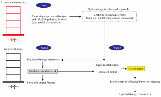
Figure 11.
The procedure of applying parametric emulators for damage identification.
Table 2.
The inputs and outputs of parametric emulators.
Applying Particle Swarm Optimization (PSO), Genetic Algorithm (GA), and Simulated Annealing (SA) algorithms, Marwala [78] investigated the performance of an ANN in the FE model updating of a beam as well as an H-shaped structure. It was observed that using the ANN surrogate model requires half of the time needed by the FE-based approach. The results also indicated that the error in the estimation of the first five natural frequencies was less than . To measure the distance between the parameters of the real structure and the model, he minimized the following cost function:
where the subscript indicates the th measured parameter; denotes the th calculated model parameter, and represent natural frequency and mode shape, respectively; is the number of modes; and are weighting factors, and stands for Modal Assurance Criterion [95].
Wang, et al. [79] trained an ANN for predicting the maximum inter-story relative displacement of a nonlinear system whose input data were the inter-story stiffnesses and the wind excitation force at the first floor and roof level. This neural network can be applied for structural assessment and health monitoring. Torkzadeh, et al. [80] presented a two-stage method for crack identification in plate-like structures. In the first stage, the damage was localized through curvature–momentum and curvature–momentum derivative damage indicators. Then, a CFNN surrogate was trained to output the frequencies by inputting the damage severities. This surrogate model was optimized with the Bat Algorithm (BA) in terms of activation function and number of neurons, and it was used to find the damage severities through an inverse optimization process with only of the data required for direct FE simulations. They minimized the cost function of the Multiple Damage Location Assurance Criterion (MDLAC), as formulated in Equation (16):
where ; ; and denote the th natural frequency of the undamaged and damaged structures, respectively; and the subscript denotes the updated parameters. They considered the first five frequencies of the structure.
Xia, et al. [81] developed two metamodels (a BPNN and a kriging model) to map the design parameters of a self-anchored bridge to its frequencies. Using a Gaussian Mutation PSO algorithm, they investigated the performance of the metamodels in damage identification of the bridge. It was observed that the ANN outperforms the kriging model in terms of accuracy and convergence speed. Their cost function is provided in Equation (17):
where and denote the th natural frequency of the damaged and updated structures, respectively.
Ghiasi, et al. [82] performed a comparative study on structural damage detection using various surrogates: BPNN, Least Square Support Vector Machines (LS-SVMs), ANFIS, RBFN, Large Margin Nearest Neighbor (LMNN), Extreme Learning Machine (ELM), Gaussian Process (GP), and Multivariate Adaptive Regression Spline. They detected the suspected elements of damage through the Modal-Strain-Energy-based Index (MSEBI), and trained the machine learning models for predicting the index. Afterwards, they solved the inverse problem of damage severity detection using the Colliding Bodies Optimization (CBO) algorithm. It was shown that the surrogates need one-twelfth of the computational time related to the direct FE-based method; RBFNN was the fastest surrogate, and the LS-SVM was the most accurate surrogate for their model. They minimized the Root Square Error of the MSEBI index (RSEMSEBI):
where and denote the damaged and updated of th element, respectively, and is the number of elements detected in the first stage. Details of MSEBI can be found in ref. [84].
Ghiasi and Ghasemi [83] established a framework for probability-based damage detection in structures using metamodels, including CFNN, LS-SVM, and kriging. In this framework, Monte Carlo Simulation (MCS) was employed to statistically address uncertainties in modeling and measurements. PSO, BA, and Ideal Gas Molecular Movement (IGMM) algorithms were used to minimize the cost function presented in the following:
The MDLAC is defined in Equation (16). According to the results, applying surrogates leads to a tenfold reduction in computational time when compared with the direct FE-based method. In a similar study, Ghasemi, et al. [84] applied the enhanced IGMM algorithm for structural damage identification of two truss structures. Using CFNN as a surrogate model for predicting frequencies, they reached an acceptable accuracy with a 93% reduction in computational time.
Sbarufatti, et al. [85] trained an ANN for mapping the crack parameters, such as the length and position, to strain field at sensor locations in an aluminum plate. They applied the surrogate model for calculating the likelihood of the Particle Filters (PF) algorithm and performing diagnosis and prognosis of fatigue in the plate. Fathnejat and Ahmadi-Nedushan [86] investigated the damage identification in a 52-bar truss and a 200-bar double-layer grid structure in two steps. They localized suspected elements with the MSEBI index, and consequently identified the damage severity through optimizing Root Mean Square Deviation (RMSD) criterion with PSO, BA, and CBO algorithms. They trained a GMDH surrogate that reduced the need for FE analyses by about 92% and required almost half of the processing time needed by CFNN. The RMSD is presented in Equation (20):
where , , and are the th parameter of the healthy, damaged, and updated model of the structure, respectively; is the number of selected parameters, including natural frequencies, diagonal elements of the modal flexibility matrix, and the mean normalized modal strain energy.
Dou, et al. [87] used an RBFN network to emulate the displacement response of a concrete dam, and applied a hybrid algorithm, PS-FWA, to quantify the damage. According to their results, the RBFN surrogate model obtains less than error, and the damage identification process needs less than half of the running time of the FE-based method. Their cost function is provided in Equation (21):
where is the number of monitored points, and and are, respectively, the displacement at th point of the damaged and updated model.
Alexandrino, et al. [88] applied ANN to predict the mean stress values on 9 points of a plate with circular holes. They defined the damage identification problem as a multi-objective optimization and implemented the NSGA-II algorithm to minimize the differences between measured and computed stresses. Using a fuzzy decision-making system, they were able to find the radius and location of the holes and concluded that this approach reduces the computational cost and enhances the identification accuracy. Their cost functions include Equation (19) and its standard deviation (Equation (22)):
where and represent the mean stress of the th point in the damaged and updated model, respectively.
Zhao and Peng [89] compared the performance of an optimized ELM with other surrogate models, such as second-order response surface, RBFN and traditional ELM. They showed that optimized ELM with Whale Optimization Algorithm (WOA) forecasts the natural frequencies of a plane truss with errors less than 0.9% and outperforms other methods. They employed the following cost function for model updating:
where is the number of selected frequencies; and denote experimental and model acceleration FRF (AFRF) data, respectively.
Torzoni, et al. [90] presented an approach for emulating the response of a concrete beam through a multi-fidelity deep LSTM network. In this approach, two datasets were generated: high-fidelity (HF) and low-fidelity (LF) datasets. They trained a network with LF datasets obtained by a reduced basis method relying on the proper orthogonal decomposition–Galerkin approach. Then, another network was trained to map the approximated LF signals to HF signals resulting from a semi-discretized FE model. They used a Bayesian framework for model updating and identification of the damage parameters via the Markov chain MCS algorithm.
Xia, et al. [92] investigated the effect of two cost functions on the accuracy of model updating of a real bridge structure emulated with a BPNN metamodel. They used GMPSO to minimize two cost functions, one of which was based on the frequencies of the main girder, and the other was based on frequencies and vertical displacements. The cost functions are provided in Equations (24) and (25):
where and denote the th frequency of the experimental and FE models, respectively; and , respectively, stand for the corresponding vertical displacement at the th point of the experimental and FE models. It was indicated that the combination of the dynamic and static responses enhances the accuracy. Xia, et al. [91] compared the performance of three metamodeling techniques—quadratic polynomial, kriging, and ANN—in model updating of a bridge structure, and minimized the cost function presented in Equation (24). They observed that the ANN is preferable to other surrogates, in terms of accuracy and efficiency.
Fakih, et al. [93] trained an ANN for predicting the lamb waves measured with a sensor on a welded plate, considering six damage parameters, such as length, width, thickness, and position components. The output was the sensed signal, recorded with a 3 MHz sampling rate. For damage quantification, they employed an approximate Bayesian framework, which led to above 95% precision for most of the damage scenarios. They chose the cosine distance metric () for comparison between real () and predicted signals ():
Using an MLP network, RBFN, and a Least Square Support Vector Machine (LS-SVM), Feng, et al. [94] developed surrogate models for predicting the Curvature Modal Rate of Change (CMRC) based on the modulus of elasticity of cable in a cable-stayed bridge. They modeled corrosion as well as fire effects, and established a probabilistic damage model of the bridge. According to their results, MLP and LS-SVM provide rapid and accurate surrogates for the condition assessment of the bridge.
4. Discussion
In this paper, we summarize research studies on the development of ANN-based surrogates for damage identification in civil structures. By utilizing these techniques, model-based SHM becomes computationally efficient. There are advantages and disadvantages to each of these paradigms. The following subsections will describe the challenges related to their practical implementation, and provide suggestions for future research.
4.1. Method Selection
There have been numerous studies conducted on ANN surrogates for SHM, as reviewed above. Several criteria should be considered when comparing developed methods, such as time complexity, accuracy, robustness, simplicity, and memory usage. These criteria can be considered either for data generation and training or for validation and testing. The weight we assign to each criterion is application-dependent, which means that we should deal with a multi-criteria decision-making problem. A real-time SHM, for example, emphasizes time issues, while in an offline application, accuracy might be more prominent. A good sample for comparing the mentioned criteria can be found in ref. [86]. The accuracy itself is presented by several metrics. In the literature, the Mean Square Error (MSE) [82,83], Root Mean Square Error (RMSE) [38,55,80,84,85,86,89], relative RMSE [44,51], R2 [55,79,89], and relative error [42,43,45,46,47,81,87,91,92] are among the most popular criteria.
4.2. Data Generation
It is often the case that time and accuracy are two conflicting criteria, which means increased accuracy will increase the required time. They are usually affected by the data generation (sampling), the network architecture, and hyperparameters. The generation of data is one of the most time-consuming components of ANN surrogates. This is particularly relevant to the identification of multiple damages, which increase the number of combinations of states and may lead to the curse of dimensionality. The numbers of training samples in the reviewed papers are listed in Table 3. Several approaches can be tailored to reduce the number of training data, and thus the amount of time required for data generation. These techniques are known as design of experiments. Most of the studies conducted Latin Hypercube Sampling (LHS) for selecting their samples [96].
Table 3.
The number of samples and reported hyperparameters of reviewed emulators.
Moreover, the number of input and output variables can be reduced through techniques such as nondimensionalization, physical reasoning, orthogonal decomposition, principal component analysis, and sensitivity analysis [97]. Modal analysis, for instance, uses the orthogonality of mode shape relationships to determine the structural response based on a weighted sum of a limited number of mode shapes; therefore, in structural response prediction, its formulations can help reduce the number of output variables. As reviewed in the refs. [82,86], an approach was established for reducing input variables based on MSEBI indicators, indicating damaged elements of structures, and reducing the computational burden. However, it is important to note that the basic MSEBI may miss some damaged elements—because of false negative error—resulting in incorrect damage identifications [98]. Hence, it is recommended to use its enhanced versions, such as the guided method introduced in ref. [99].
4.3. Hyperparameters
Time and accuracy factors can also be improved by hyperparameter tuning. The main hyperparameters to tune are the topology of the network, the type of activation functions, optimizer, learning rate, and the number of epochs. Several neural architecture search algorithms, based on reinforcement learning [100], metaheuristics [101], and Bayesian optimization [102], have been proposed for designing the optimal or near-optimal topology of neurons in an automated manner to reach a proper performance. The reported hyperparameters in the reviewed papers are presented in Table 3. In parentheses, the numbers indicate the number of neurons ranging from inputs (left) to outputs (right).
4.4. Overfitting
In ANNs, we should take care of both underfitting (poor performance on training data) and overfitting (performing well on training data, but failing on new data). It is believed that overfitting occurs when the model learns the noise in training data and fails to generalize the learned patterns to unseen data. An established robust method to address overfitting is called cross-validation, in which the trained model is evaluated and tuned on different subsets of data [103].
4.5. Noise
Another important issue in SHM is the noise, which is an inevitable part of any real-world application. There are three main types of structures discussed in the literature: numerical, lab-scale, and real. In numerical simulations, the noise in data is defined as a random number with a Gaussian or uniform distribution [85,90]. Despite what may seem to be an accurate method in numerical examples, it may not be robust in real structures. Compared to real structures, noise is often controlled and lower in lab-scale structures. Hence, the best way to ensure that methods perform well is to test them in real-world structures. In addition to noise issues, testing in a real-world environment can reveal other advantages and disadvantages of the techniques.
4.6. Model Development
When constructing a numerical model of an experimental structure, it is necessary to calibrate the model to ensure that it is consistent with the experiment [90,91]. In this regard, architectural drawings and design codes can be used to initialize the model, and then stiffness, material properties, support conditions, etc., should be updated to reflect actual conditions. The drawings of old and historical structures might be unavailable or incomplete, which means that simulation results would not match the reality. It is also possible for the model and real structure to differ when high damage occurs and induces nonlinearity, or when the type of damage is different from the one assumed. For such cases, robust methods that do not heavily rely on models are desirable. Combining these methods with vision-based or nondestructive approaches is an interesting idea for future research.
4.7. Novel ANNs and Techniques
Although traditional ANNs show satisfactory performance in most of the reviewed papers, they are prone to being brittle when the training data are small or do not capture the mechanical relationships in structures. Additionally, they usually fail to extrapolate well when they are tested on new data out of the distribution of training samples. Therefore, it is recommended to use modern ANNs, such as Graph Neural Networks [104] and PINNs [26], which incorporate the physics of the problem. A combination of different types of ANNs, such as hybridizing PINN with LSTM (PhyLSTM) [53], or combining BNN and PINN (B-PINN) [105], can be implemented easily with the available software packages. Furthermore, a combination of PINN with NAS techniques can lead to the discovery of application-oriented neural topologies. With regard to this, designing and training specific networks for typical structures, such as shear frames, trusses, and bridges, can be highly impactful. They can reduce the need for large datasets, save training time, and improve the performance of ANNs in other related applications through transfer learning [106]. The basic idea of transfer learning is that some parts of networks obtained in a pre-trained model can be used in another model with some fine tuning to perform similar tasks.
4.8. Software and Hardware
Nowadays, there are many machine learning packages through which ANNs as well as the mentioned metrics and techniques can be easily implemented. As examples, TensorFlow, PyTorch, scikit-learn, and Theano are some of the most popular ML libraries available as open source [52,53,57,90]. Simulating structures is usually achieved by coding with programming languages such as Python or MATLAB [81,93], or using simulation software such as ETABS, SAP 2000 [42,43], ANSYS [55,81,89,91,92,94], LS-Dyna, and ABAQUS [52,93].
There are numerous matrix multiplications involved with ANN training, which can be performed in parallel. The availability of advanced hardware such as Graphics Processing Units (GPUs) and Tensor Processing Units (TPUs) allows for the acceleration of ANNs, especially for deep models. For advanced applications, programming platforms, such as Compute Unified Device Architecture (CUDA), which provide direct access to GPUs for the execution of such parallel tasks and optimizing memory usage, can be utilized.
5. Conclusions
SHM systems analyze the condition of civil infrastructures to determine the possible defects, thereby ensuring the safety and integrity of structures. In this regard, ANNs, as promising tools for learning and modeling complex relationships, have drawn considerable attention from researchers and engineers. In this literature review, we have particularly concentrated on their application as surrogate models for structures.
The surrogates are divided into two general classes: parametric and nonparametric. The nonparametric models are typically fed with external factors (such as loading or acceleration), and predict the response of structures. On the other hand, parametric models involve some attributions from structural models (such as sectional area and modulus of elasticity). It is observed that, in the literature, there has recently been a shift in popularity from nonparametric surrogates to parametric ones. The nonparametric models generally rely on the time domain, which makes them prone to noise and synchronization issues. Nonetheless, they are suitable for near-real-time damage identification because there is no need for an expensive identification process. In the literature, these surrogates are commonly supplemented with another parametric surrogate (PENN) to detect damage. Nonetheless, due to numerous combinations of damage, PENNs cannot cover all damage states in large structures. The parametric models usually need an optimization module to identify the damage, but they commonly provide higher levels of identification (presence, location, and severity). This optimization task is performed by a metaheuristic algorithm, which requires some time for processing the damage identification. Therefore, they are appropriate for offline applications. Additionally, it is observed that the damage is usually simulated as a reduction in stiffness, while the change in other structural parameters, such as mass, damping, and geometry, have not received enough attention. In the following, a few directions for future studies are recommended to help address such challenges and lay the foundation for their application in real-world projects:
- Developing accurate surrogates considering nonlinear and realistic mechanical models of structural systems.
- Applying autoencoder networks to extract new reliable features with less sensitivity against noise.
- Improving the robustness of surrogates through generative adversarial networks and reinforcement learning.
- Developing interpretable and physics-informed surrogates, instead of black box models, to provide human-understandable insights for their output.
- Establishing fast optimizers for both training ANNs and inverse damage identification to increase their applicability for real-time tasks.
- Data fusion in various levels ranging from input data to identification results based on Bayesian and fuzzy inference systems.
- Developing new types of sensors equipped with modern technologies, such as the Internet of Things, to prevent inputting invalid data into the models.
Author Contributions
Conceptualization, A.D.E. and S.H.; methodology, A.D.E. and S.H.; software, A.D.E.; validation, A.D.E. and S.H.; formal analysis, A.D.E. and S.H.; investigation, A.D.E.; resources, A.D.E. and S.H.; data curation, A.D.E. and S.H.; writing—original draft preparation, A.D.E.; writing—review and editing, A.D.E. and S.H.; visualization, A.D.E.; supervision, S.H.; project administration, S.H.; funding acquisition, S.H. All authors have read and agreed to the published version of the manuscript.
Funding
This work was supported by the National Natural Science Foundation of China under Grant No. 11672108 and 11911530692.
Data Availability Statement
Not applicable.
Conflicts of Interest
The authors declare no conflict of interest.
References
- Yön, B.; Sayın, E.; Onat, O. Earthquakes and structural damages. In Earthquakes-Tectonics, Hazard and Risk Mitigation; InTech: London, UK, 2017; pp. 319–339. [Google Scholar] [CrossRef]
- Fan, W.; Qiao, P. Vibration-based Damage Identification Methods: A Review and Comparative Study. Struct. Health Monit. 2011, 10, 83–111. [Google Scholar] [CrossRef]
- Agdas, D.; Rice, J.A.; Martinez, J.R.; Lasa, I.R. Comparison of Visual Inspection and Structural-Health Monitoring As Bridge Condition Assessment Methods. J. Perform. Constr. Facil. 2016, 30, 04015049. [Google Scholar] [CrossRef]
- Dong, C.-Z.; Catbas, F.N. A review of computer vision–based structural health monitoring at local and global levels. Struct. Health Monit. 2021, 20, 692–743. [Google Scholar] [CrossRef]
- Farrar, C.R.; Doebling, S.W. An Overview of Modal-Based Damage Identification Methods; Los Alamos National Laboratory: Los Alamos, NM, USA, 1997. [Google Scholar]
- Hou, R.; Xia, Y. Review on the new development of vibration-based damage identification for civil engineering structures: 2010–2019. J. Sound Vib. 2021, 491, 115741. [Google Scholar] [CrossRef]
- Sudret, B.; Marelli, S.; Wiart, J. Surrogate models for uncertainty quantification: An overview. In Proceedings of the 2017 11th European Conference on Antennas and Propagation (EUCAP), Paris, France, 19–24 March 2017; pp. 793–797. [Google Scholar]
- Cheng, K.; Lu, Z.; Ling, C.; Zhou, S. Surrogate-assisted global sensitivity analysis: An overview. Struct. Multidiscip. Optim. 2020, 61, 1187–1213. [Google Scholar] [CrossRef]
- Forrester, A.I.J.; Keane, A.J. Recent advances in surrogate-based optimization. Prog. Aerosp. Sci. 2009, 45, 50–79. [Google Scholar] [CrossRef]
- ADELI, H.; YEH, C. Perceptron Learning in Engineering Design. Comput.-Aided Civ. Infrastruct. Eng. 1989, 4, 247–256. [Google Scholar] [CrossRef]
- Xie, Y.; Ebad Sichani, M.; Padgett, J.E.; DesRoches, R. The promise of implementing machine learning in earthquake engineering: A state-of-the-art review. Earthq. Spectra 2020, 36, 1769–1801. [Google Scholar] [CrossRef]
- Flah, M.; Nunez, I.; Ben Chaabene, W.; Nehdi, M.L. Machine Learning Algorithms in Civil Structural Health Monitoring: A Systematic Review. Arch. Comput. Methods Eng. 2021, 28, 2621–2643. [Google Scholar] [CrossRef]
- Toh, G.; Park, J. Review of Vibration-Based Structural Health Monitoring Using Deep Learning. Appl. Sci. 2020, 10, 1680. [Google Scholar] [CrossRef]
- Akinosho, T.D.; Oyedele, L.O.; Bilal, M.; Ajayi, A.O.; Delgado, M.D.; Akinade, O.O.; Ahmed, A.A. Deep learning in the construction industry: A review of present status and future innovations. J. Build. Eng. 2020, 32, 101827. [Google Scholar] [CrossRef]
- Avci, O.; Abdeljaber, O.; Kiranyaz, S.; Hussein, M.; Gabbouj, M.; Inman, D.J. A review of vibration-based damage detection in civil structures: From traditional methods to Machine Learning and Deep Learning applications. Mech. Syst. Signal Process. 2021, 147, 107077. [Google Scholar] [CrossRef]
- Bishop, C.M. Neural networks and their applications. Rev. Sci. Instrum. 1994, 65, 1803–1832. [Google Scholar] [CrossRef]
- Rumelhart, D.E.; Hinton, G.E.; Williams, R.J. Learning representations by back-propagating errors. Nature 1986, 323, 533–536. [Google Scholar] [CrossRef]
- Pinkus, A. Approximation theory of the MLP model in neural networks. Acta Numer. 1999, 8, 143–195. [Google Scholar] [CrossRef]
- Voulodimos, A.; Doulamis, N.; Doulamis, A.; Protopapadakis, E. Deep Learning for Computer Vision: A Brief Review. Comput. Intell. Neurosci. 2018, 2018, 7068349. [Google Scholar] [CrossRef]
- Ghosh, J.; Nag, A. An Overview of Radial Basis Function Networks. In Radial Basis Function Networks 2: New Advances in Design; Howlett, R.J., Jain, L.C., Eds.; Physica-Verlag HD: Heidelberg, Germany, 2001; pp. 1–36. [Google Scholar]
- Renisha, G.; Jayasree, T. Cascaded Feedforward Neural Networks for speaker identification using Perceptual Wavelet based Cepstral Coefficients. J. Intell. Fuzzy Syst. 2019, 37, 1141–1153. [Google Scholar] [CrossRef]
- Kondo, T.; Kondo, C.; Takao, S.; Ueno, J. Feedback GMDH-type neural network algorithm and its application to medical image analysis of cancer of the liver. Artif. Life Robot. 2010, 15, 264–269. [Google Scholar] [CrossRef]
- Guang-Bin, H.; Qin-Yu, Z.; Chee-Kheong, S. Extreme learning machine: A new learning scheme of feedforward neural networks. In Proceedings of the 2004 IEEE International Joint Conference on Neural Networks (IEEE Cat. No.04CH37541), Budapest, Hungary, 25–29 July 2004; Volume 982, pp. 985–990. [Google Scholar]
- Buntine, W. Bayesian back-propagation. Complex Syst. 1991, 5, 603–643. [Google Scholar]
- Hochreiter, S.; Schmidhuber, J. Long Short-Term Memory. Neural Comput. 1997, 9, 1735–1780. [Google Scholar] [CrossRef]
- Raissi, M.; Perdikaris, P.; Karniadakis, G.E. Physics-informed neural networks: A deep learning framework for solving forward and inverse problems involving nonlinear partial differential equations. J. Comput. Phys. 2019, 378, 686–707. [Google Scholar] [CrossRef]
- Wong, F.S.; Thint, M.P.; Tung, A.T. On-Line Detection of Structural Damage Using Neural Networks. Civ. Eng. Syst. 1997, 14, 167–197. [Google Scholar] [CrossRef]
- Chandrashekhara, K.; Okafor, A.C.; Jiang, Y.P. Estimation of contact force on composite plates using impact-induced strain and neural networks. Compos. Part B Eng. 1998, 29, 363–370. [Google Scholar] [CrossRef]
- Huang, C.S.; Hung, S.L.; Wen, C.M.; Tu, T.T. A neural network approach for structural identification and diagnosis of a building from seismic response data. Earthq. Eng. Struct. Dyn. 2003, 32, 187–206. [Google Scholar] [CrossRef]
- Xu, B.; Wu, Z.; Yokoyama, K. A localized identification strategy with neural networks and its application to structural health monitoring. J. Struct. Eng. JSCE A 2002, 48, 419–427. [Google Scholar]
- Wu, Z.; Xu, B.; Yokoyama, K. Decentralized Parametric Damage Detection Based on Neural Networks. Comput.-Aided Civ. Infrastruct. Eng. 2002, 17, 175–184. [Google Scholar] [CrossRef]
- Xu, B.; Wu, Z.; Yokoyama, K. A Post-Seismic Damage Detection Strategy in Time Domain for a Suspension Bridge with Neural Networks. J. Appl. Mech. 2003, 6, 1149–1156. [Google Scholar] [CrossRef]
- Faravelli, L.; Casciati, S. Structural damage detection and localization by response change diagnosis. Prog. Struct. Eng. Mater. 2004, 6, 104–115. [Google Scholar] [CrossRef]
- Kim, K.-B.; Yoon, D.-J.; Jeong, J.-C.; Lee, S.-S. Determining the stress intensity factor of a material with an artificial neural network from acoustic emission measurements. NDT E Int. 2004, 37, 423–429. [Google Scholar] [CrossRef]
- Jiang, X.; Adeli, H. Dynamic Wavelet Neural Network for Nonlinear Identification of Highrise Buildings. Comput.-Aided Civ. Infrastruct. Eng. 2005, 20, 316–330. [Google Scholar] [CrossRef]
- Xu, B.; Wu, Z.; Yokoyama, K.; Harada, T.; Chen, G. A soft post-earthquake damage identification methodology using vibration time series. Smart Mater. Struct. 2005, 14, S116–S124. [Google Scholar] [CrossRef]
- Xu, B. Time Domain Substructural Post-Earthquake Damage Diagnosis Methodology with Neural Networks; Springer: Berlin/Heidelberg, Germany, 2005; pp. 520–529. [Google Scholar]
- Xu, B.; Du, T. Direct Substructural Identification Methodology Using Acceleration Measurements with Neural Networks; SPIE: San Diego, CA, USA, 2006; Volume 6178. [Google Scholar]
- Xu, B.; Chen, G.; Wu, Z.S. Parametric Identification for a Truss Structure Using Axial Strain. Comput.-Aided Civ. Infrastruct. Eng. 2007, 22, 210–222. [Google Scholar] [CrossRef]
- Jiang, X.; Adeli, H. Pseudospectra, MUSIC, and dynamic wavelet neural network for damage detection of highrise buildings. Int. J. Numer. Methods Eng. 2007, 71, 606–629. [Google Scholar] [CrossRef]
- Mita, A.; Qian, Y. Damage Indicator for Building Structures Using Artificial Neural Networks as Emulators; SPIE: San Diego, CA, USA, 2007; Volume 6529. [Google Scholar]
- Wang, W.; Chen, G.; Hartnagel, B. Real-Time Condition Assessment of the Bill Emerson Cable-Stayed Bridge Using Artificial Neural Networks; SPIE: San Diego, CA, USA, 2007; Volume 6529. [Google Scholar]
- Wang, W.; Chen, G. System Identification of a Highway Bridge from Earthquake-Induced Responses Using Neural Networks. In Structural Engineering Research Frontiers; ASCE: Long Beach, CA, USA, 2007; pp. 1–12. [Google Scholar] [CrossRef]
- Qian, Y.; Mita, A. Acceleration-based damage indicators for building structures using neural network emulators. Struct. Control Health Monit. 2008, 15, 901–920. [Google Scholar] [CrossRef]
- Xu, B. Inverse Analysis for Identification of a Truss Structure with Incomplete Vibration Strain. In Proceedings of the World Forum on Smart Materials and Smart Structures Technology; CRC Press: Boca Raton, FL, USA, 2008; p. 260. [Google Scholar]
- Choo, J.F.; Ha, D.H.; Koh, H.M. A Neural Network-Based Damage Detection Algorithm Using Dynamic Responses Measured in Civil Structures. In Proceedings of the 2009 Fifth International Joint Conference on INC, IMS and IDC, Seoul, Republic of Korea, 25–27 August 2009; pp. 682–685. [Google Scholar]
- Xu, B.; Song, G.; Masri, S.F. Damage detection for a frame structure model using vibration displacement measurement. Struct. Health Monit. 2012, 11, 281–292. [Google Scholar] [CrossRef]
- Mitchell, R.; Kim, Y.; El-Korchi, T. System identification of smart structures using a wavelet neuro-fuzzy model. Smart Mater. Struct. 2012, 21, 115009. [Google Scholar] [CrossRef]
- Khalid, M.; Yusof, R.; Joshani, M.; Selamat, H.; Joshani, M. Nonlinear Identification of a Magneto-Rheological Damper Based on Dynamic Neural Networks. Comput. Aided Civ. Infrastruct. Eng. 2014, 29, 221–233. [Google Scholar] [CrossRef]
- Jiang, X.; Mahadevan, S.; Yuan, Y. Fuzzy stochastic neural network model for structural system identification. Mech. Syst. Signal Process. 2017, 82, 394–411. [Google Scholar] [CrossRef]
- Perez-Ramirez, C.A.; Amezquita-Sanchez, J.P.; Valtierra-Rodriguez, M.; Adeli, H.; Dominguez-Gonzalez, A.; Romero-Troncoso, R.J. Recurrent neural network model with Bayesian training and mutual information for response prediction of large buildings. Eng. Struct. 2019, 178, 603–615. [Google Scholar] [CrossRef]
- Vega, M.A.; Todd, M.D. A variational Bayesian neural network for structural health monitoring and cost-informed decision-making in miter gates. Struct. Health Monit. 2022, 21, 4–18. [Google Scholar] [CrossRef]
- Zhang, R.; Liu, Y.; Sun, H. Physics-informed multi-LSTM networks for metamodeling of nonlinear structures. Comput. Methods Appl. Mech. Eng. 2020, 369, 113226. [Google Scholar] [CrossRef]
- Shukla, K.; Di Leoni, P.C.; Blackshire, J.; Sparkman, D.; Karniadakis, G.E. Physics-Informed Neural Network for Ultrasound Nondestructive Quantification of Surface Breaking Cracks. J. Nondestruct. Eval. 2020, 39, 61. [Google Scholar] [CrossRef]
- Xue, J.; Xiang, Z.; Ou, G. Predicting single freestanding transmission tower time history response during complex wind input through a convolutional neural network based surrogate model. Eng. Struct. 2021, 233, 111859. [Google Scholar] [CrossRef]
- Li, S.; Li, S.; Laima, S.; Li, H. Data-driven modeling of bridge buffeting in the time domain using long short-term memory network based on structural health monitoring. Struct. Control Health Monit. 2021, 28, e2772. [Google Scholar] [CrossRef]
- Tan, X.; Chen, W.; Zou, T.; Yang, J.; Du, B. Real-time prediction of mechanical behaviors of underwater shield tunnel structure using machine learning method based on structural health monitoring data. J. Rock Mech. Geotech. Eng. 2022. [Google Scholar] [CrossRef]
- Trifunac, M.D. Comparisons between ambient and forced vibration experiments. Earthq. Eng. Struct. Dyn. 1972, 1, 133–150. [Google Scholar] [CrossRef]
- Kirikera, G.R.; Shinde, V.; Schulz, M.J.; Ghoshal, A.; Sundaresan, M.; Allemang, R. Damage localisation in composite and metallic structures using a structural neural system and simulated acoustic emissions. Mech. Syst. Signal Process. 2007, 21, 280–297. [Google Scholar] [CrossRef]
- Yan, W.-J.; Chronopoulos, D.; Papadimitriou, C.; Cantero-Chinchilla, S.; Zhu, G.-S. Bayesian inference for damage identification based on analytical probabilistic model of scattering coefficient estimators and ultrafast wave scattering simulation scheme. J. Sound Vib. 2020, 468, 115083. [Google Scholar] [CrossRef]
- Nazarko, P.; Ziemiański, L. Application of artificial neural networks in the damage identification of structural elements. Comput. Assist. Methods Eng. Sci. 2017, 18, 175–189. [Google Scholar]
- Nazarko, P. Soft computing methods in the analysis of elastic wave signals and damage identification. Inverse Probl. Sci. Eng. 2013, 21, 945–956. [Google Scholar] [CrossRef]
- Nazarko, P.; Ziemiański, L. Novelty detection based on elastic wave signals measured by different techniques. Comput. Assist. Methods Eng. Sci. 2017, 19, 317–330. [Google Scholar]
- Lu, Y.; Ye, L.; Su, Z.; Zhou, L.; Cheng, L. Artificial Neural Network (ANN)-based Crack Identification in Aluminum Plates with Lamb Wave Signals. J. Intell. Mater. Syst. Struct. 2009, 20, 39–49. [Google Scholar] [CrossRef]
- Xu, Y.; Jin, R. Measurement of reinforcement corrosion in concrete adopting ultrasonic tests and artificial neural network. Constr. Build. Mater. 2018, 177, 125–133. [Google Scholar] [CrossRef]
- Ziaja, D.; Nazarko, P. SHM system for anomaly detection of bolted joints in engineering structures. Structures 2021, 33, 3877–3884. [Google Scholar] [CrossRef]
- Liu, S.W.; Huang, J.H.; Sung, J.C.; Lee, C.C. Detection of cracks using neural networks and computational mechanics. Comput. Methods Appl. Mech. Eng. 2002, 191, 2831–2845. [Google Scholar] [CrossRef]
- Han, X.; Xu, D.; Liu, G.R. A computational inverse technique for material characterization of a functionally graded cylinder using a progressive neural network. Neurocomputing 2003, 51, 341–360. [Google Scholar] [CrossRef]
- Araújo, A.L.; Mota Soares, C.M.; Herskovits, J.; Pedersen, P. Parameter estimation in active plate structures using gradient optimisation and neural networks. Inverse Probl. Sci. Eng. 2006, 14, 483–493. [Google Scholar] [CrossRef]
- Rautela, M.; Gopalakrishnan, S.; Gopalakrishnan, K.; Deng, Y. Ultrasonic Guided Waves Based Identification of Elastic Properties Using 1D-Convolutional Neural Networks. In Proceedings of the 2020 IEEE International Conference on Prognostics and Health Management (ICPHM), Detroit, MI, USA, 8–10 June 2020; pp. 1–7. [Google Scholar]
- De Fenza, A.; Sorrentino, A.; Vitiello, P. Application of Artificial Neural Networks and Probability Ellipse methods for damage detection using Lamb waves. Compos. Struct. 2015, 133, 390–403. [Google Scholar] [CrossRef]
- Qian, C.; Ran, Y.; He, J.; Ren, Y.; Sun, B.; Zhang, W.; Wang, R. Application of artificial neural networks for quantitative damage detection in unidirectional composite structures based on Lamb waves. Adv. Mech. Eng. 2020, 12, 1687814020914732. [Google Scholar] [CrossRef]
- Liu, G.R.; Han, X.; Ohyoshi, T. Computational Inverse Techniques for Material Characterization Using Dynamic Response. Int. J. Soc. Mater. Eng. Resour. 2002, 10, 26–33. [Google Scholar] [CrossRef]
- Liu, G.R.; Han, X.; Xu, Y.G.; Lam, K.Y. Material characterization of functionally graded material by means of elastic waves and a progressive-learning neural network. Compos. Sci. Technol. 2001, 61, 1401–1411. [Google Scholar] [CrossRef]
- Nazarko, P. Axial force prediction based on signals of the elastic wave propagation and artificial neural networks. MATEC Web Conf. 2019, 262, 10009. [Google Scholar] [CrossRef][Green Version]
- Nazarko, P.; Ziemianski, L. Force identification in bolts of flange connections for structural health monitoring and failure prevention. Procedia Struct. Integr. 2017, 5, 460–467. [Google Scholar] [CrossRef]
- Nazarko, P.; Ziemiański, L. Application of Elastic Waves and Neural Networks for the Prediction of Forces in Bolts of Flange Connections Subjected to Static Tension Tests. Materials 2020, 13, 3607. [Google Scholar] [CrossRef] [PubMed]
- Marwala, T. Finite-element-model Updating Using the Response-surface Method. In Finite-Element-Model Updating Using Computional Intelligence Techniques: Applications to Structural Dynamics; Springer: London, UK, 2010; pp. 103–125. [Google Scholar]
- Wang, V.Z.; Ginger, J.D.; Henderson, D.J. A Surrogate Model for a Type of Nonlinear Hysteretic System with Application to Wind Response Analysis. In Proceedings of the 2013 World Congress on Advances in Structural Engineering and Mechanics (ASEM13), Jeju, Republic of Korea, 8–12 September 2013. [Google Scholar]
- Torkzadeh, P.; Fathnejat, H.; Ghiasi, R. Damage detection of plate-like structures using intelligent surrogate model. Smart Struct. Syst 2016, 18, 1233–1250. [Google Scholar] [CrossRef]
- Xia, Z.; Li, A.; Li, J.; Duan, M. Comparison of hybrid methods with different meta model used in bridge model-updating. Balt. J. Road Bridge Eng. 2017, 12, 193–202. [Google Scholar] [CrossRef]
- Ghiasi, R.; Ghasemi, M.R.; Noori, M. Comparative studies of metamodeling and AI-Based techniques in damage detection of structures. Adv. Eng. Softw. 2018, 125, 101–112. [Google Scholar] [CrossRef]
- Ghiasi, R.; Ghasemi, M.R. Optimization-based method for structural damage detection with consideration of uncertainties-a comparative study. Smart Struct. Syst 2018, 22, 561–574. [Google Scholar] [CrossRef]
- Ghasemi, M.R.; Ghiasi, R.; Varaee, H. Probability-Based Damage Detection of Structures Using Surrogate Model and Enhanced Ideal Gas Molecular Movement Algorithm; Springer: Cham, Germany, 2018; pp. 1657–1674. [Google Scholar]
- Sbarufatti, C.; Cadini, F.; Locatelli, A.; Giglio, M. Surrogate modelling for observation likelihood calculation in a particle filter framework for automated diagnosis and prognosis. In Proceedings of the EWSHM 2018 9th European Workshop on Structural Health Monitoring (EWSHM 2018), Manchester, UK, 10–13 July 2018; pp. 1–12. [Google Scholar]
- Fathnejat, H.; Ahmadi-Nedushan, B. An efficient two-stage approach for structural damage detection using meta-heuristic algorithms and group method of data handling surrogate model. Front. Struct. Civ. Eng. 2020, 14, 907–929. [Google Scholar] [CrossRef]
- Dou, S.-q.; Li, J.-j.; Kang, F. Health diagnosis of concrete dams using hybrid FWA with RBF-based surrogate model. Water Sci. Eng. 2019, 12, 188–195. [Google Scholar] [CrossRef]
- Alexandrino, P.d.S.L.; Gomes, G.F.; Cunha, S.S. A robust optimization for damage detection using multiobjective genetic algorithm, neural network and fuzzy decision making. Inverse Probl. Sci. Eng. 2020, 28, 21–46. [Google Scholar] [CrossRef]
- Zhao, Y.; Peng, Z. Frequency Response Function-Based Finite Element Model Updating Using Extreme Learning Machine Model. Shock Vib. 2020, 2020, 8526933. [Google Scholar] [CrossRef]
- Torzoni, M.; Manzoni, A.; Mariani, S. Health Monitoring of Civil Structures: A MCMC Approach Based on a Multi-Fidelity Deep Neural Network Surrogate. Comput. Sci. Math. Forum 2022, 2, 16. [Google Scholar] [CrossRef]
- Xia, Z.; Li, A.; Feng, D.; Li, J.; Chen, X.; Zhou, G. Comparative analysis of typical mathematical modelling methods through model updating of a real-life bridge structure with measured data. Measurement 2021, 174, 108987. [Google Scholar] [CrossRef]
- Xia, Z.; Li, A.; Shi, H.; Li, J. Model updating of a bridge structure using vibration test data based on GMPSO and BPNN: Case study. Earthq. Eng. Eng. Vib. 2021, 20, 213–221. [Google Scholar] [CrossRef]
- Fakih, M.A.; Chiachío, M.; Chiachío, J.; Mustapha, S. A Bayesian approach for damage assessment in welded structures using Lamb-wave surrogate models and minimal sensing. NDT E Int. 2022, 128, 102626. [Google Scholar] [CrossRef]
- Feng, J.; Gao, K.; Gao, W.; Liao, Y.; Wu, G. Machine learning-based bridge cable damage detection under stochastic effects of corrosion and fire. Eng. Struct. 2022, 264, 114421. [Google Scholar] [CrossRef]
- Allemang, R.J. A correlation coefficient for modal vector analysis. In Proceedings of the 1st International Modal Analysis Conference, Orlando, FL, USA, 8–10 November 1982; pp. 110–116. [Google Scholar]
- McKay, M.D.; Beckman, R.J.; Conover, W.J. A Comparison of Three Methods for Selecting Values of Input Variables in the Analysis of Output From a Computer Code. Technometrics 2000, 42, 55–61. [Google Scholar] [CrossRef]
- Viana, F.A.C.; Gogu, C.; Haftka, R.T. Making the Most Out of Surrogate Models: Tricks of the Trade. Int. Des. Eng. Tech. Conf. Comput. Inf. Eng. Conf. 2010, 44090, 587–598. [Google Scholar]
- Kaveh, A.; Rahmani, P.; Dadras Eslamlou, A. A Multistage Damage Detection Approach Using Graph Theory and Water Strider Algorithm. Iran. J. Sci. Technol. Trans. Civ. Eng. 2022, 46, 33–54. [Google Scholar] [CrossRef]
- Kaveh, A.; Rahmani, P.; Dadras Eslamlou, A. Guided Water Strider Algorithm for Structural Damage Detection Using Incomplete Modal Data. Iran. J. Sci. Technol. Trans. Civ. Eng. 2022, 46, 771–788. [Google Scholar] [CrossRef]
- Jaafra, Y.; Luc Laurent, J.; Deruyver, A.; Saber Naceur, M. Reinforcement learning for neural architecture search: A review. Image Vis. Comput. 2019, 89, 57–66. [Google Scholar] [CrossRef]
- Liu, Y.; Sun, Y.; Xue, B.; Zhang, M.; Yen, G.G.; Tan, K.C. A Survey on Evolutionary Neural Architecture Search. IEEE Trans. Neural Netw. Learn. Syst. 2021, 1–21. [Google Scholar] [CrossRef] [PubMed]
- White, C.; Neiswanger, W.; Savani, Y. BANANAS: Bayesian Optimization with Neural Architectures for Neural Architecture Search. Proc. AAAI Conf. Artif. Intell. 2021, 35, 10293–10301. [Google Scholar] [CrossRef]
- Picard, R.R.; Cook, R.D. Cross-Validation of Regression Models. J. Am. Stat. Assoc. 1984, 79, 575–583. [Google Scholar] [CrossRef]
- Scarselli, F.; Gori, M.; Tsoi, A.C.; Hagenbuchner, M.; Monfardini, G. The Graph Neural Network Model. IEEE Trans. Neural Netw. 2009, 20, 61–80. [Google Scholar] [CrossRef]
- Yang, L.; Meng, X.; Karniadakis, G.E. B-PINNs: Bayesian physics-informed neural networks for forward and inverse PDE problems with noisy data. J. Comput. Phys. 2021, 425, 109913. [Google Scholar] [CrossRef]
- Tan, C.; Sun, F.; Kong, T.; Zhang, W.; Yang, C.; Liu, C. A Survey on Deep Transfer Learning; Springer: Cham, Germny, 2018; pp. 270–279. [Google Scholar]


Publisher’s Note: MDPI stays neutral with regard to jurisdictional claims in published maps and institutional affiliations. |
© 2022 by the authors. Licensee MDPI, Basel, Switzerland. This article is an open access article distributed under the terms and conditions of the Creative Commons Attribution (CC BY) license (https://creativecommons.org/licenses/by/4.0/).