A Spatially Varying Ground Motion Model with an Evolving Energy Spectrum

Abstract

Besides phase variability, amplitude variability is one of the two manifestations of the spatially varying ground motion (SVGM) in the frequency domain. Neglecting the amplitude variability of the earthquake spectra can result in an underestimation of the structural responses. Few existing amplitude variability models can be used for estimating spectra at a distance from a reference location. In this paper, a new amplitude variability model describing the evolution of the energy spectra is developed based on records of five earthquake events acquired from the SMART 1 array. The similarity between the spectra of two locations is used as a metric for measuring the spectrum changes. The energy spectra at a distance from a reference location are found to be composed of two parts, including the averaged spectra and the random variation part. In the new model, the former is estimated by the moving average of the reference spectrum, while the envelope of the latter is approximated by the wavelet approximation of the reference spectrum’s Fourier amplitude spectrum. The parameters of five models for each event and a general model for all five events are identified. Monte Carlo simulations are used for testing the models. The results validate the new model in terms of capturing the similarity changes of actual earthquakes.

1. Introduction

The study of the ground motion model has long been emphasized by researchers [1,2,3]. Due to the complex propagation process of earthquakes through their path, the frequency contents of the ground motion vary as traveling. Considering the spatially varying ground motion (SVGM) is important in designing [4], seismic assessment [5], and the design of control systems [6,7] for long-span bridges. The SVGM can be described by the phase and amplitude variability in the frequency domain. A lot of arrays have been used in studying the SVGM, such as the SMART 1 array [8,9], LSST array [10], Chiba array [11], UPSAR array [12], Argostoli array [13], etc.

Phase variability, which is usually described as the changes in coherence with the varying separation distance, has been extensively studied by researchers. [14,15,16,17] Harichandran [14] proposed an empirical coherence model based on the records from the SMART 1 array. Hao, Oliveira [16] proposed a model with a simplified function form based on the analysis of the SMAR1 array records. Abrahamson, Schneider [15] used the inverse hyperbolic tangent function of the coherence instead of directly fitting the coherences estimated from the LSST array. By using this approach, the residue of the hyperbolic tangent transformed the coherence, exhibiting a Gaussian distribution. Cui and Hong [17] extended the coherence model into the time-frequency domain by using S-transform [18] and short-time Fourier transform [19].

Studies on amplitude variability are relatively scarce. Schneider, Stepp [20] proposed an amplitude variability model of the Fourier amplitude spectrum (FAS) based on the ground motion record obtained from the LSST array, assuming the amplitude of the FAS exhibited a log-normal distribution. Zerva and Zervas [21] proposed using an envelope for describing the amplitude variability of ground motions. Ancheta, Stewart [22] examined the model by records obtained from the Borrego Valley Differential Array in Canada. However, these models mainly emphasize describing the statistical features of the spectral amplitude variability. To the knowledge of the authors, no study has shown whether these models are feasible in estimating the earthquake spectra and whether the estimated spectra have similar properties as the real earthquakes.

Existing models utilize the Fourier spectra to describe the amplitude variability of the ground motion in the frequency domain. The model introduced by Schneider, Stepp [20] modeled the amplitude variability of the Fourier spectra with the standard deviation of their logarithmic differences. With this model, many researchers [22,23,24,25,26] studied the amplitude variability of records acquired from different strong-motion dense arrays, such as the UPSAR array [23], SK-net data [24], LSST array [22], Argostoli array [26], etc. In the models using logarithmic differences of the Fourier spectra, the insignificant changes in energy between a relatively small level and an even smaller level can also result in a large value, overestimating the spectral amplitude variability as a result. Another amplitude variability model proposed by Zerva and Zervas [21] utilized the direct differences of the Fourier spectra which prevent the problem in Schneider’s model of using logarithmic difference. These models focus on describing the statistical characteristics, but none of them have been used for estimating the spectra of adjacent locations from a reference spectrum, and none of them have been used for artificial earthquake generation.

Using the Fourier-spectrum-based amplitude variability model leads to a problem in generating artificial earthquakes. When generating artificial ground motions, power spectral density (PSD) is more widely used than the Fourier spectrum. In Fourier-spectrum-based models, additive random numbers are added to the Fourier spectrum, resulting in the amplitude variability of the PSD being proportional to the amplitude of the reference spectrum. As is demonstrated later in this paper, this phenomenon is not consistent with the actual records. Therefore, in this paper, the amplitude variability is modeled with the energy spectra of the ground motions. In this way, The PSD and the corresponding Fourier spectrum in the adjacent locations can be easily acquired from the energy spectra.

In this paper, the similarity between the energy spectra of two locations is used as a metric to measure spectral changes. The similarity changes of five earthquake events acquired from the SMART 1 array are studied. A new amplitude variability model based on energy spectra is proposed. In this model, the energy spectra differences are assumed to be band-wise proportional to the low-frequency wavelet approximation of the reference Fourier spectrum and are modeled with colored Gaussian noise. The evolution process of the average spectrum that is a certain distance from the reference location can be equivalent to smoothing the reference Fourier spectrum with a moving window function. A general parametric model for the horizontal components of the five events is also given. Monte Carlo simulations are used for testing the amplitude variability model and the general parametric model.

2. Similarity Changes in the Energy Spectra

Most of the existing SVGM models consider only coherence changes [27], and few of them consider the evolution of spectra. When the soil conditions are identical, the spectra at different locations are usually assumed to be the same. In this way, the spectral features of earthquakes as a whole can be modeled in a statistical sense, such as the Clough–Penzien spectrum [28] or evolutionary spectral models [29,30]. However, in civil engineering, estimating adjacent spectra from a reference spectrum is usually a concern, especially when artificial ground motions in a random field are to be generated.

In this section, five events from the SMART 1 array on Taiwan Island are re-explored. The records are obtained from the PEER NGA-WEST2 database. The metadata of these five events are listed in

Table 1. Metadata of earthquakes.

Event	Year	Magnitude	Mechanism	${\mathit{R}}_{\mathit{j}\mathit{b}} \left(\mathbf{km}\right)$
SMART1(5)	1981	5.9	Reverse	25.50
SMART1(25)	1983	6.5	Reverse	95.57
SMART1(33)	1985	5.8	Normal	41.53
SMART1(40)	1986	6.32	Reverse	58.69
SMART1(45)	1986	7.3	Reverse	56.01

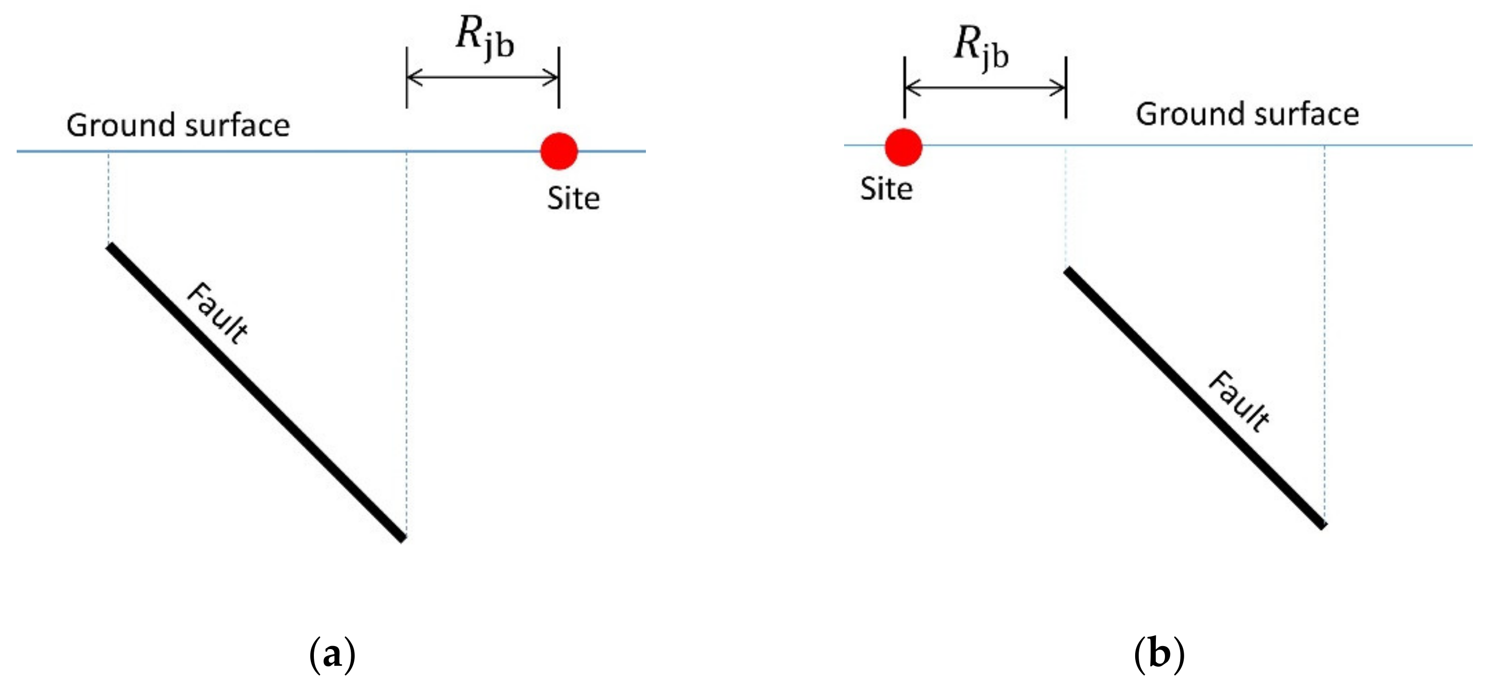
. The moment magnitude is used to measure the intensity of the earthquake, and $R_{jb}$ stands for the Joyner–Boore distance [31] to the rupture plane, which is the shortest distance from a site to the surface projection of the rupture plane, as shown in Figure 1. Four of the five events originated from the reverse mechanism. In this study, the ground motions are analyzed within each event; therefore, the normal mechanism is also included in the analysis.

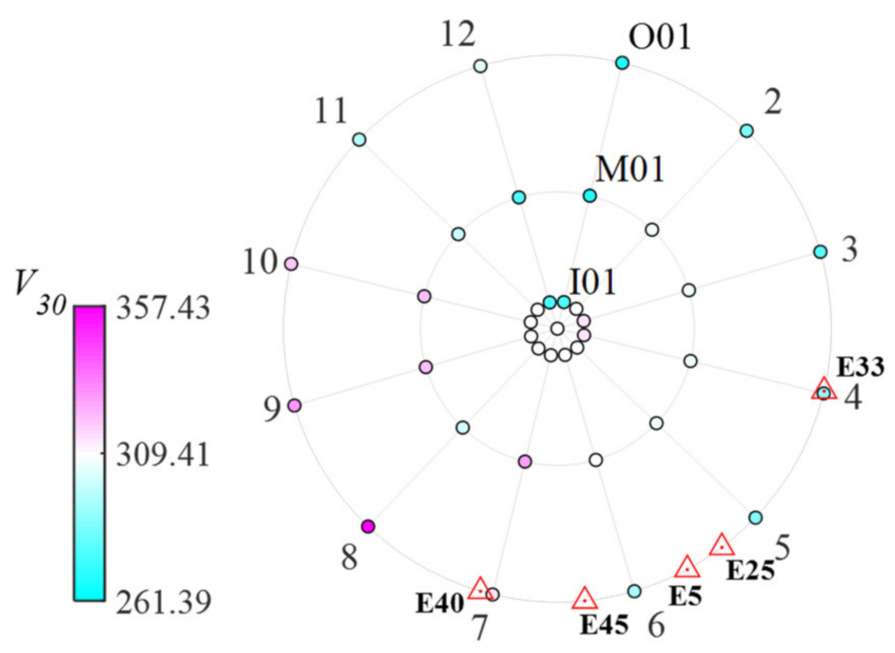
The layout of the SMART1 array is shown in Figure 2. The records are from 37 stations, consisting of 1 center station C00 and the other 36 stations. The diameters of these three loops are 400 m, 2 km, and 4 km, respectively. Three loops are formed by the 36 stations, and each loop has 12 stations. The stations are labeled by I, M, or O, followed by numbers. The numbers at the rim of Figure 2 represent the station number; for example, 3 represents the direction of the I-03, M-03, and O-03 stations. In Figure 2, the average shear velocity of the top 30 m $V_{S,30}$ of different stations is marked with circles of different colors. The range of the soil shear wave velocity is from 267.67 m/s and 357.43 m/s. The variation of $V_{S,30}$ is relatively small, and the soil condition of all the stations falls into soil category C, as stipulated in the European Code [32]. Figure 2 also marks the incident direction of the earthquakes relative to the central station with triangles. Further information about the SMART-1 array can be found in [8,33].

The changes in the energy spectra are measured by a similarity variable ${\varsigma }_{jk}$, as shown in Equation (1). ${\varsigma }_{jk}$ stands for the similarity between the energy spectra of locations $j$ and $k$.

$${\varsigma }_{jk}=\frac{{\displaystyle \sum _{k=0}^{n_f}\left[S_{jj,0}(f_i)S_{kk,0}(f_i)\right]}}{\sqrt{{\displaystyle \sum _{k=0}^{n_f}{S}_{jj,0}^2(f_i)}{\displaystyle \sum _{k=0}^{n_f}{S}_{kk,0}^2(f_i)}}}$$

(1)

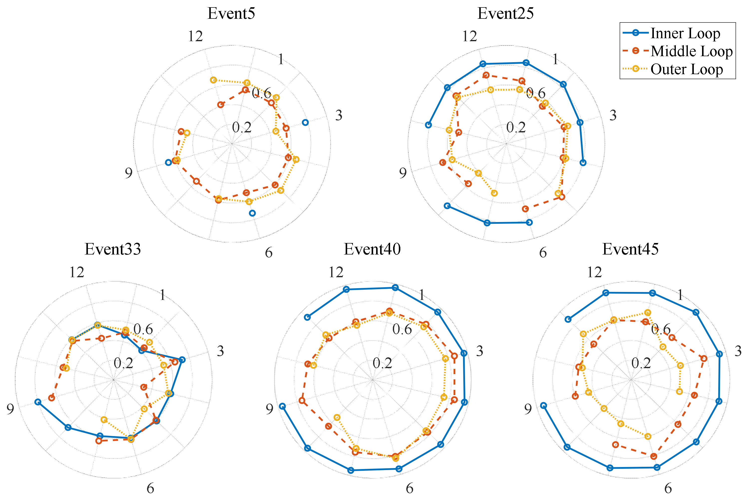
The energy spectrum of location $j$ is defined as $S_{jj,0}(f_i)={\left|U_j(f_i)\right|}^2$, the subscript 0 means no smoothing is carried out in calculating the energy spectrum, and $U(f)={\displaystyle {\int }_{-\infty }^{+\infty }u(t)e^{-i2\pi ft}dt}$ is the Fourier spectrum of the time series $u(t)$. Figure 3 shows the similarity of the energy spectrum between the center station and the other stations.

The results of the E-W components are shown in Figure 3; the N-S and the vertical components show a similar trend as the E-W components, except that the similarities of the vertical components are obviously smaller than those of the horizontal components.

Some of the records in these five events are not available from the database, such that the lines in Figure 3 are not closed. Figure 4 shows four conditions of unavailable records for different loops.

For simplicity, the earthquakes are categorized by events and directions; for example, the E-W components of the event SMART1(45) are abbreviated as Event 45EW, the N-S component is abbreviated as NS, and the vertical component is abbreviated as DN. Each category is called an earthquake group.

As is shown in Figure 3, the varying trend of similarities differs significantly among different events. For Events 25, 40, and 45, the similarities decrease with the increase in separation distance. When the distance is 200 m, most of the similarities are above 0.9; similarities fall rapidly to around 0.6 when the distance reaches 1 km and change slowly to 2 km. However, for Events 5 and 33, the similarities change rapidly after 200 m of propagation and reach a relatively steady value until 2 km. The lowest similarity values of Events 5 and 33 are, on average, smaller than those of Events 25, 40, and 45.

As analyzed before, the changes in soil properties in the SMART 1 array are relatively small. In inspecting the similarity changes of all the earthquake groups, there is little indication that the similarity is related to the variation of the soil shear wave velocities, the azimuth direction, the earthquake magnitude, the duration, and the epicenter distance. This phenomenon is consistent with several previous studies. [8,27,33,34,35]. Therefore, in the following context, several assumptions are made and are listed as follows. The influence of the azimuth direction is ignored; the propagation of the ground motion is assumed to be isotropy; and the influence of the magnitude, duration, and epicenter distance of the earthquake is ignored.

In this study, the characteristics of the ground motions are studied both ring-wise and pair-wise. When a statistical value is obtained ring-wise, the separation distances increase with the increase in the ring radius, while, when it is studied pair-wise, each pair of data is categorized by their separation distances, and the statistical value is calculated in each category.

The spectral similarities in different loops are averaged. The average similarities of the middle loop ${\overline{\varsigma }}_M$ and the outer loop ${\overline{\varsigma }}_O$ are expressed as a function of the average similarity of the inner loop ${\overline{\varsigma }}_I$ and are shown in Figure 5a. In this figure, the average similarities of the horizontal and the vertical components are plotted separately. The superscripts $h$ and $v$ represent the variables corresponding to the horizontal and vertical components, respectively.

In Figure 5a, all the lines show an increasing trend with the increase in ${\overline{\varsigma }}_I$, indicating that the values of ${\overline{\varsigma }}_M$ and ${\overline{\varsigma }}_O$ are related to the value of ${\overline{\varsigma }}_I$. Different components in the same earthquake event have different similarity values; hence, in the following analysis, different components of one ground motion are considered separately.

The spectral similarities between all the station pairs are calculated, and the similarities of the station pairs with the same separation distance are averaged. The varying trend of the similarities with respect to the separation distance is shown in Figure 5b. Except that the average similarities of Event 25DN are at the same level as the horizontal components, the average similarities of the vertical components in the other events are all smaller than those of the horizontal components. All the similarities decrease with the increase in separation distance. In Events 5 and 33, the average similarities reach a relatively stable value at around 0.4, which is also the lower bound of all the similarities. It is obvious in Figure 5b that the smaller the similarity at the distance of 103.53 m is, the faster the similarities decrease with the increase in the separation distance.

The influence of unavailable records is studied. The middle loop of Event 40 possesses all 12 records and is therefore used to study the influence of unavailable data on the similarity estimation. Four conditions, as shown in Figure 4, are studied. The results for the EW components of Event 40 are shown in Figure 6. For each condition, unavailable data at different locations are calculated and compared with the result calculated by all the records. The maximum standard deviationw of each condition for the other components are listed in

Table 2. Maximum standard deviations for different conditions of unavailable records.

Conditions	EW	NS	DN
1	0.0174	0.0283	0.0153
2	0.0390	0.0371	0.0261
3	0.0231	0.0436	0.0266
4	0.0780	0.0741	0.0382

. For each condition, unavailable data at different locations are calculated and compared with the result calculated by all the records.

As shown in Figure 6 and Table 2, the difference between the full records and records with unavailable data increases with the increase in the number of unavailable records. However, the difference is relatively small and is much smaller than the fluctuation in similarities with the variations in separation distances, as shown in Figure 5. Consequently, the influence of unavailable records is neglected in this study.

To find a proper way of estimating the similarity dropping, the energy spectra of the center station are first examined. The smoothed spectra of the horizontal components are shown in Figure 7.

An obvious trend can be observed in Figure 7, the rate of the similarity dropping is related to the spectral energy between 0 and 4 Hz. The larger the spectral energy is, the slower the similarities drop. In engineering practice, ${\overline{\varsigma }}_I$ cannot be easily acquired; thus, a variable $E_r$ is defined to approximate the behavior of ${\overline{\varsigma }}_I$.

$$E_r=\frac{\sqrt{{\displaystyle {\int }_0^4{S}_{rr,0}(f)df}}}{w_{95}}$$

(2)

where the subscript $r$ in $E_r$ stands for the reference spectrum. When the spectrum of the center station is used as the reference spectrum, the subscript is replaced with $C$; $w_{95}$ is the bandwidth of the 95% total energy calculated from 0 Hz. The relationship between $E_C$ and the average similarity of the inner loop ${\overline{\varsigma }}_I$ is shown in Figure 8. In this figure, abbreviations are used for different earthquake groups; for example, $E_{45}^N$ stands for Event 45NS, and the superscripts $N$, $E$, and $v$ stand for the N-S components, the E-W components, and the vertical components, respectively.

As shown in Figure 8, the horizontal components ${\overline{\varsigma }}_I$ increase monotonically with the increase in $E_C$, showing that $E_C$ is a good indicator of the variation in ${\overline{\varsigma }}_I$. The same is true for the vertical components. As is shown later in this paper, the spectral amplitude variability of the vertical components is at a different level from the horizontal components; these two categories are presented separately. In the following context, ${\overline{\varsigma }}_I$ is proved to be related to the evolution characteristics of the average spectrum, and then $E_r$ is used instead of ${\overline{\varsigma }}_I$.

3. Model of the Evolutionary Energy Spectra

After showing the similarity changes of the earthquake, in this section, a new amplitude variability model that can capture the similarity changes of the earthquakes is established.

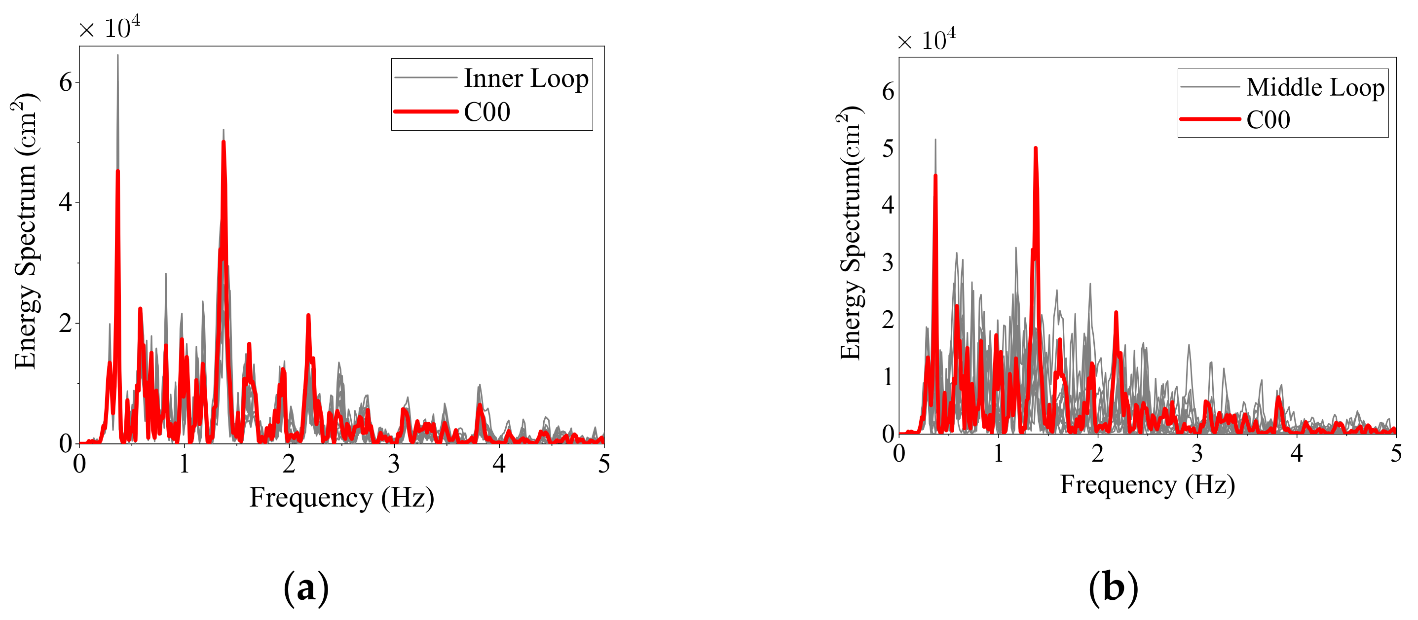
In Figure 9, the energy spectrum of the center station in Event 45EW is used as a reference and compared with the spectra of the inner loop and the middle loop, respectively. As shown in Figure 9, when the distance increases from 200 m to 1000 m, the variability of the spectrum increases. The energy of the earthquake spreads to the adjacent frequency ranges where the reference spectrum has small energy.

A ground motion signal is composed of many segments, each segment going through different paths. The versatility of the path and incident angle is the reason that the standard deviation of the spectrum differences is not proportional to the reference spectrum but rather proportional to a curve that covers the energy distribution of a large number of ground motions in a large region. This curve can be estimated by fitting the Clough–Penzien spectrum [28], but the Clough–Penzien spectrum cannot fit all the spectrum shapes in different earthquakes. The estimation of earthquake spectra within the engineering scale is a more local process. A more feasible way is to smooth the energy spectrum, but the smoothed spectrum has large energy near the large spikes of the reference spectrum but underestimates the energy changes at the other frequency ranges. In this study, the square of the low-frequency wavelet Fourier spectrum approximation is found to be a good approximation to this curve and is used for estimating the standard deviation of the energy changes.

The energy spectrum differences between any nonrepetitive location pairs $D_s(d_{ij},f)=S_{ii,0}(f)-S_{jj,0}(f)$ are calculated and categorized by different separation distances $d_{ij}$. The statistical distribution of $D_s(f)$ has an approximately zero mean but a very larger kurtosis, from 4 to 10, and larger tails than the Gaussian distribution. However, the signed square root of $D_F(f)=sign\left(D_s\right)\sqrt{\left|D_s\right|}$ has a kurtosis at around 3 and can be approximated by the Gaussian random process band-wise in the frequency domain, as shown in Equation (3).

$$D_F(f)=p(d_{rj},f)W\left(U_r(f)\right)\xi (f)$$

(3)

$p(d_{rj},f)$ is a band-wise constant scale parameter, $W\left(U_r(f)\right)$ represents the low-frequency wavelet approximation of the Fourier spectrum $U_r(f)$, and $\xi (f)$ is a zero-mean random process following the normal distribution.

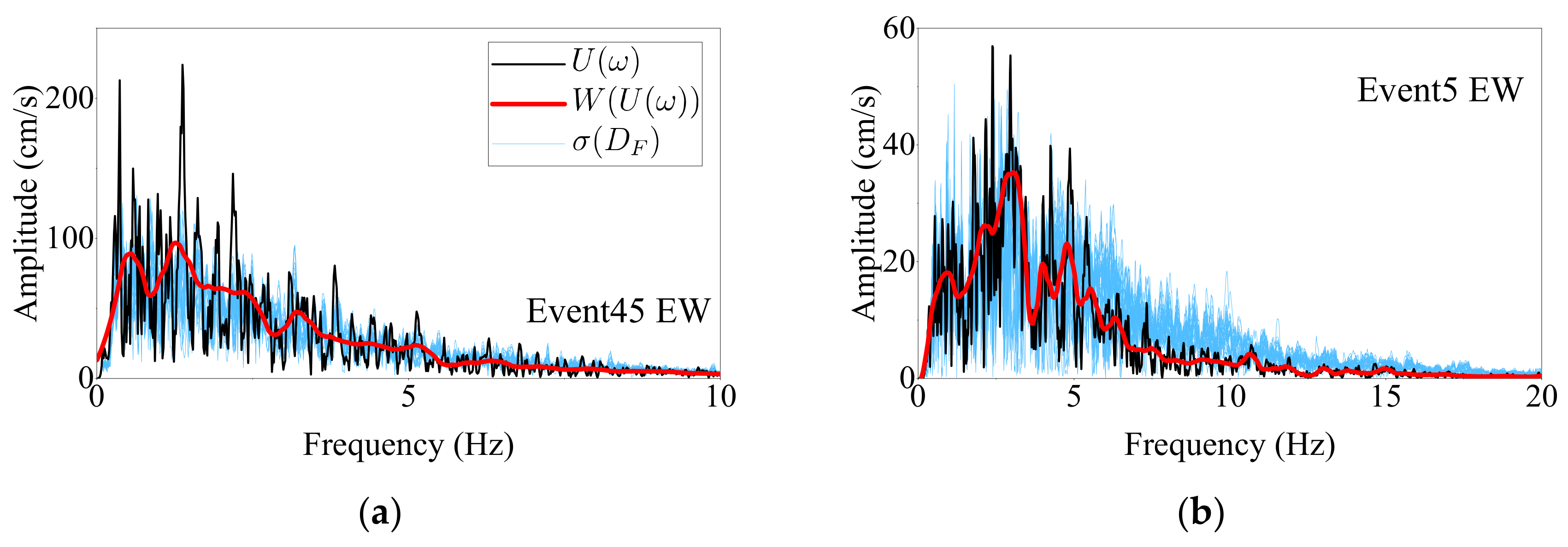
The reference Fourier spectrum $U_r(f)$, low-frequency wavelet approximation $W\left(U_r(f)\right)$, and standard deviation of $D_F(f)$, $\sigma \left(D_F\right)$, corresponding to Event 45EW and Event 5EW are compared in Figure 10a,b. The widely used Daubechies 4 wavelet function [36] is used for the low-frequency wavelet approximation. The frequency resolution of the energy spectra is 1.53 × 10⁻³ Hz, and the eighth-level wavelet approximation is used as the low-frequency wavelet approximation. $\sigma \left(D_F\right)$ is calculated frequency-wise using the spectra pairs with the same separation distance. As shown in Figure 10a,b, $\sigma \left(D_F\right)$ is not proportional to the reference Fourier spectrum, whereas the low-frequency wavelet approximation is a good approximation of the varying trend of $\sigma \left(D_F\right)$.

By removing the wavelet approximation from the deviation, the results, $\sigma (D_F)/W(U_r)$, of Event 45EW and Event 5EW are presented in gray lines in Figure 10c,d. In Figure 10c, $\sigma (D_F)/W(U_r)$ stays constant from 0.2 Hz to around 5 Hz and increases at around 5 Hz to another constant value until 10 Hz. A similar trend can also be observed in Figure 10d. The $\sigma (D_F)/W(U_r)$ of Event 5EW is more rugged than that of Event 45EW, showing that the low-frequency wavelet approximation is not a perfect estimation of the spectral differences. However, as is proved later in this paper, assuming $\sigma (D_F)/W(U_r)$ to be band-wise constant is accurate enough for capturing the main feature of real spectral similarity changes.

Then, the energy spectrum $S_{d_{rj},0}(f)$ at a certain distance $d_{rj}$ away from the reference location can be expressed as follows.

$$S_{d_{rj},0}(f)=\left|\frac{1}{\sqrt{2}}sign\left[\xi (f)\right]{\left(p(d_{rj},f)W\left(U_r(f)\right)\xi (f)\right)}^2+{\overline{S}}_{d_{rj},0}(d_{rj},f)\right|$$

(4)

where ${\overline{S}}_{d_{rj},0}(\omega )$ stands for the average spectrum $d_{rj}$ away from the reference location, and $sign\left[\xi (f)\right]$ is the sign of the random variable $\xi (f)$. In Equation (4), the energy spectrum consists of two parts: the first part describes the variation in differences between the reference spectrum and the estimated spectrum, and the second part describes the change in the average spectrum with respect to the separation distance. In the following context, the models of $p(d_{rj},f)$ and ${\overline{S}}_{d_{rj},0}(d_{rj},f)$ are established with the five groups of SMART-1 records listed in Table 1 to capture their similarity changes.

After analyzing the energy spectra of all the records, the aforementioned frequency bands in $p(d_{rj},f)$ are set as [0.2, 4] Hz, [4, 8] Hz, [8, 11] Hz, and [11, 50] Hz. Subscripts from 1 to 4 are assigned to $p(d_{rj},f)$, e.g., $p_1(d_{rj})$, to distinguish the value of $p(d_{rj},f)$ in different frequency ranges. The average value of $p(d_{rj},f)$ in each band is calculated. The results of $p_1(d_{rj})$ for the horizontal components are shown in Figure 11.

As shown in Figure 11, all the lines have similar peaks and troughs at the same separation distance, which might involve a certain mechanism that is not within the scope of this study. All the lines have an increasing trend with the increase in distance; the lines corresponding to Events 5, 25, and 33 reach their steady value, whereas those for Events 40 and 45 keep on increasing. The ordering of the increasing rate of the lines in Figure 11 is roughly the same as the rate of spectral similarity dropping. The difference is that the increasing rate is closer for the components in one event. In the left three figures of Figure 11, the lines have similar increasing rates but different amplitudes. According to the line shapes in Figure 11, $p(d_{rj},f)$ is assumed to have the form of Equation (5).

$$p(d_{rj},f)=\left\{\begin{array}{ll}{p}_1(d_{rj})=C_{13}\left[1-\exp (-C_{12}{d}_{rj}{}^{C_{11}})\right],\hfill & f\in [0.2, 4]\mathrm{Hz}\hfill \\ p_2,\hfill & f\in (4, 8]\mathrm{Hz}\hfill \\ p_3,\hfill & f\in (8, 11]\mathrm{Hz}\hfill \\ p_4,\hfill & f\in (11, 50]\mathrm{Hz}\hfill \end{array}\right.$$

(5)

$C_{11}$, $C_{12}$, and $C_{13}$ are parameters that depend on the separation distance $d_{rj}$; $p_2$, $p_3$, and $p_4$ are the mean values of $\sigma (D_F)/W(U_r)$ in the corresponding frequency range.

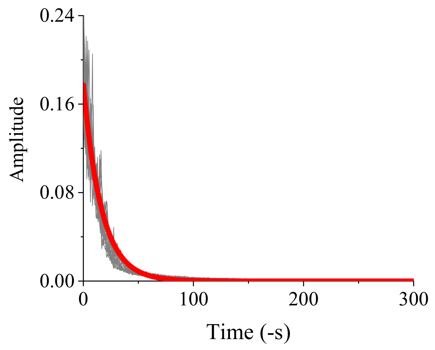
Extract a stationary section of $D_F(f)/W(U_r)$ from each record and Fourier transform these frequency domain series to another $\tau$ domain, where $\tau =-t$. The $\tau$ domain is called the negative-time domain in this paper, and the corresponding spectrum is called the negative-time spectrum. The negative-time spectra of $D_F(f)/W(U_r)$ of different records overlap with each other, showing that the negative-time spectrum is not affected by the separation distance. The negative-time spectra in different earthquake groups are averaged and drawn in gray lines in Figure 12.

Obviously, all the gray lines have similar shapes. An exponent function $N(\tau )$ in Equation (6) is used to describe the negative-time spectrum of $D_F(f)/W(U_r)$, and $C_f$ is the amplitude parameter controlling the power of $D_F(f)/W(U_r)$. The fitted $N(\tau )$ is plotted in a bold red solid line in Figure 12.

$$N(\tau )=C_f\exp (-0.12{\tau }^{0.8})$$

(6)

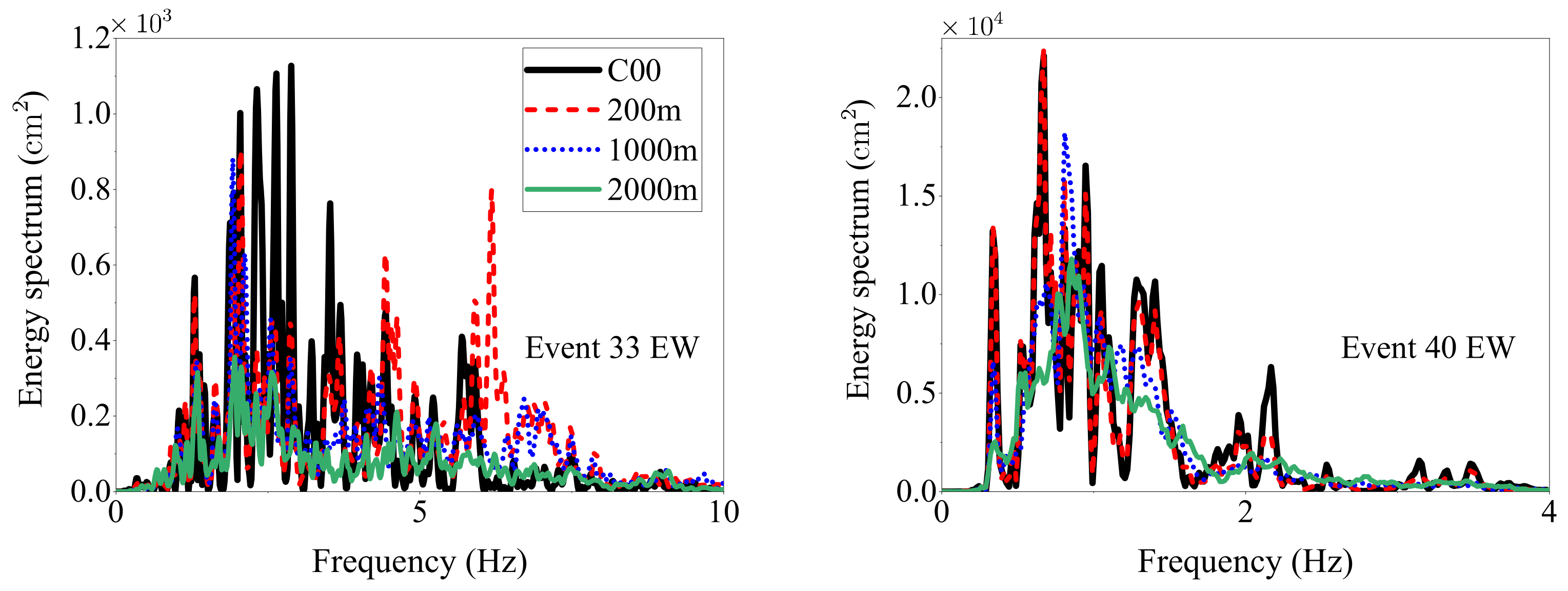
The evolution process of the average spectrum is another important part of the spectral amplitude variability. The averaged spectrum of Event 33EW and 40EW of the three array loops are compared with the spectrum of the center station in Figure 13.

As shown in Figure 13, because the versatility of the propagation paths of earthquakes increases with the increase in separation distance, the earthquake energy spreads more evenly within its frequency bandwidth as the separation distance increases. The average spectra of Event 33EW vary more significantly than those of Event 40EW and drop to an energy level closer to zero. The average spectra of Event 40EW retain more features of the center station energy spectrum. The evolution speeds of the average spectrum are different for different earthquake groups.

In this study, the evolution process of the average spectrum is simulated by averaging the reference Fourier spectrum with a moving Gaussian window. The Fourier spectrum is used rather than the energy spectrum because, when moving-averaging the former spectrum, the energy spreads faster than the latter, especially when the energy is already evenly spread to some extent. The expression of this Gaussian window is shown in Equation (7).

$$w(f)=C_s\exp \left[-{\left(\raisebox{1ex}{$f$}\!\left/ \!\raisebox{-1ex}{$\beta $}\right.\right)}^2\right]$$

(7)

where $C_s=1/{\displaystyle {\int }_{-\infty }^{\infty }\exp \left[-{\left(f/\beta \right)}^2\right]}df$ is a normalization parameter, $\beta$ is a parameter that controls the bandwidth of the window. To identify the equivalent energy spreading process such that the similarity dropping traces between the estimated earthquake spectra and the reference spectrum are the same, as shown in Figure 5b, the spectra of the center station in each earthquake group are used as a reference. The realizations of a spectrum that is a certain distance from the reference spectrum is calculated by Equation (4). $p(d_{rj},f)$ in Equation (5) is identified by the nonlinear least square (NLS) method. The colored noise $\xi (f)$ in Equation (4) satisfies the negative-time spectrum of Equation (6). Monte Carlo simulation is used to calculate the similarity between the reference spectrum and the realized spectrum. A simple searching method is used to find the optimal window width so that the similarity is the same as the corresponding real earthquake. For each separation distance and each earthquake group, 10,000 simulations are used to calculate the expectation value of the similarity.

The expectation value estimated by the Monte Carlo simulation changes when different groups of random values are used. As a result, traditional optimization methods are not feasible for searching for the optimal value of $\beta$. The most simple approach is to grid search all the possible values of $\beta$, which is computationally costly. A good alternative is to use an adaptive grid search, which uses a relatively coarse grid at first and then shrinks the grid until the tolerance of error is reached. The values of $\beta$ for the horizontal components are searched and shown in Figure 14.

In Figure 14, the natural logarithm of the parameter $\beta$ increases with the separation distance and the increasing rate, and the shapes of the lines are different for different earthquake groups. Linear increasing trends can be observed in the long tails of Events 5, 25, and 33; thus, Equation (8) is used to describe the evolution of $\beta$.

$$\beta (d_{rj})=\exp \left\{C_{23}\left[1-\exp \left(-C_{22}{d}_{rj}{}^{C_{21}}\right)\right]+C_{24}{d}_{rj}-C_{25}\right\}$$

(8)

where $C_{21}$, $C_{22}$, and $C_{23}$ are parameters that vary for different earthquake groups; $C_{24}$ and $C_{25}$ are assumed to be constant and are identified to be 1.25 × 10⁻⁴ and 7, respectively.

To test the amplitude variability model given in Equation (4), the parameters in Equations (5) and (8) are identified for each earthquake group by the NLS method. With the identified spectral difference model and the average spectrum model, the mean similarities of the energy spectrum model realized by Equation (4) are then calculated again by Monte Carlo simulation. The results for the EW components are compared with the real similarities in Figure 15.

As shown in Figure 15, the similarities realized by the novel amplitude variability model fit very well with the real similarities. The results for the NS components are also as good as those of the EW components. The results for the vertical components are discussed separately in Section 5 Alhough Event 33 has a normal mechanism, it exhibits similar properties as the other events. The simulation results show that the new model can be used for simulating the regional evolutionary process of the earthquake spectra.

The fitting error $E_f$ is defined in Equation (9) to measure the performance of fitting.

$$E_f=\left|{\varsigma }_f-{\varsigma }_d\right|$$

(9)

where ${\varsigma }_f$ and ${\varsigma }_d$ represent the fitted similarity and the similarity of the actual earthquake. The results of $E_f$ for different events and directions are listed in

Table 3. Fitting error for different events and directions.

Direction	Event 5	Event 25	Event 33	Event 40	Event 45
EW	0.099	0.061	0.073	0.044	0.065
NS	0.061	0.066	0.072	0.102	0.082

. As listed in this table, all the fitted results show a high accuracy, with the maximum fitting accuracy of 0.102 being much smaller than the fluctuation in similarity curves of actual ground motions.

4. A General Parametric Model for the SMART-1 Horizontal Components

In this section, a general parametric amplitude variability model is proposed for the five events of the SMART 1 records.

First, $p(d_{rj},f)$ is studied. According to the nonlinear least square results of $p_1(d_{rj})$, the parameters of $p_1(d_{rj})$ are more similar within one event; besides the properties of $E_r$, the larger the bandwidth of the spectrum, the faster $p_1(d_{rj})$ increases. Thus, a new variable $E_1$ is defined for the parametric model in Equation (10). Compared with $E_r$, the main body of Equation (2) is retained, but four times the energy in the higher frequency range [4, $w_{95}$] Hz is subtracted as a penalty factor in the numerator.

$$E_1=\frac{\sqrt{{\displaystyle {\int }_0^4{S}_{rr,0}(f)df}}-4\sqrt{{\displaystyle {\int }_4^{w_{95}}{S}_{rr,0}(f)df}}}{w_{95}}$$

(10)

According to the function form of Equation (5), when different values are assigned to $C_{11}$, the optimal value of the parameter $C_{12}$ can change significantly, and the optimal value of $C_{13}$ also changes with the values of $C_{11}$ and $C_{12}$. Therefore, the optimal value of $C_{11}$ is first fitted according to the NLS results. The fitted value of $C_{11}$ is then substituted as known parameters to identify the optimal value of $C_{12}$ by the NLS methods. After acquiring the fitted value of $C_{12}$, NLS methods are carried out again with the newly identified parameters of $C_{11}$ and $C_{12}$ to identify the optimal value of $C_{13}$. Thus, these three parameters are identified sequentially from $C_{11}$ to $C_{12}$ and, further, to $C_{13}$. The values identified by the NLS method in each step and the general parametric model are shown in Figure 16.

Compare Figure 16 and Figure 11. The larger $E_1$ is, the flatter the $p_1(d_{rj})$ is. Using $E_1$ as the independent variable, the parameters for the general $p_1(d_{rj})$ are identified in Equation (11). The function forms in Equation (11) are chosen, not only aiming at acquiring a good fitting of the shapes but also depending on the understanding of the parameters’ developing trend outside the fitting range.

$$\begin{array}{l}{C}_{11}=0.26+6.32\times {10}^{-2}{E}_1+0.1\exp (-40E_1{}^3)\\ C_{12}=0.18\exp (-1.8{(E_1+0.27)}^2)(1+erf(16(E_1+0.27)))+\frac{0.15}{\pi }\arctan (10(E_1-0.2)+\pi /2)\\ C_{13}=-0.718E_1{}^3+1.35E_1{}^2+0.336E_1+0.874\end{array}$$

(11)

In Figure 16, $C_{11}$ decreases with the increase in $E_1$. According to the sign of $E_1$, the feature of the parameters can mainly be divided into two groups; when $E_1$ < 0, $C_{11}$ decreases rapidly, and when $E_1$ > 0, $C_{11}$ decreases slowly. The value of $C_{12}$ should be larger than 0, according to the behavior of $C_{12}$ in Figure 16; when $E_1$ < 0, $C_{12}$ should approach zero as $E_1$ approaches $-\infty$. With the increase in $E_1$, $C_{12}$ increases rapidly from zero. The value of $C_{12}$ decreases slowly and approaches 0.15 with the increase in $E_1$. The constraints on the parameter $C_{13}$ are relatively loose; thus, a good fitting of the varying trend is considered at first, and a simple function form is picked. When $E_1$ < 0, $C_{13}$ decreases, whereas when $E_1$ > 0, $C_{13}$ increases, and a third-order polynomial function is fitted.

$p_2$, $p_3$, and $p_4$ barely change with the separation distance and are less important compared with $p_1(d_{rj})$; thus, they are assumed to be constant. Because the energy in the frequency range higher than 4 Hz is relatively smaller, the spectrum in this frequency range is more susceptible to noises. The reliability of the identified values of these three parameters depends on how much the reference spectrum can reflect the feature of the spectra in the considered area. When the bandwidth of the reference spectrum is obviously smaller than the other spectra, $p_2$, $p_3$, and $p_4$ can be underestimated, and vice versa. 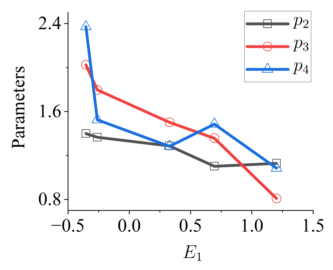Thus, the values of $p_2$, $p_3$, and $p_4$ are identified event-wise rather than component-wise, and the values of $p_2$, $p_3$, and $p_4$ identified from the records for the horizontal components are averaged and shown in Figure 17.

As shown in Figure 17, the values of $p_2$, $p_3$, and $p_4$ decrease with the increase in $E_1$. Linear functions are used to fit $p_2$. The energy at the frequency range of $p_3$ and $p_4$ is relatively small and have little influence on the similarity changes; thus, they are expressed as multiples of $p_2$. The general models for $p_2$, $p_3$, and $p_4$ are shown in Equation (12).

$$\begin{array}{l}{p}_2=-0.19E_1+1.32\\ p_3=1.18p_2\\ p_4=1.22p_2\end{array}$$

(12)

As is depicted in Figure 14, $E_r$ is a good indicator for describing the variation in $\beta$ and is thus used as the variable of the parameters in Equation (8). $\beta$ has a similar function form as $p_1(d_{rj})$; thus, the parameters of $\beta$ follow the same process as $p_1(d_{rj})$ and are identified sequentially from $C_{21}$ to $C_{22}$ and to $C_{23}$. The values identified by the NLS method and the general parametric model are shown in Figure 18.

As shown in Figure 18, the identified values of $C_{21}$, $C_{22}$, and $C_{23}$ can roughly be separated into two groups according to the value of $E_r$. The function form of $C_{21}$, $C_{22}$, and $C_{23}$ need to fit the varying trend of these three parameters and at the same time guarantee the rationality of the parameters when extrapolation is required. As a result, exponent functions, which have upper and lower bounds when $E_r$ > 0, are used. The general parametric model for the parameter $\beta$ in Equation (8) is also identified and shown in Equation (13). To better fit the parameters, large exponent values appear in Equation (13).

$$\begin{array}{l}{C}_{21}=0.45+0.95exp(-1.57\times {10}^2{E}_r{}^5)\\ C_{22}=5.2\times {10}^{-2}-5.13\times {10}^{-2}exp(-1.78\times {10}^3{E}_r{}^9)\\ C_{23}=7+0.9exp(-0.11E_r{}^{14})\end{array}$$

(13)

The similarity changes described by the general parametric model are computed by Monte Carlo simulation, as in the previous section, and are compared with the real similarity changes in Figure 19. As shown in Figure 19, the general parametric model can capture the main features of the similarity changes in real earthquakes.

The fitting error $E_f$ is also calculated for the general model. The results are listed in

Table 4. Fitting error for different events and directions of the general model.

Direction	Event 5	Event 25	Event 33	Event 40	Event 45
EW	0.081	0.075	0.092	0.066	0.066
NS	0.088	0.092	0.096	0.143	0.136

.

Comparing Table 4 with Table 3, the fitting errors of the general model are all larger than those of the separate models, with the largest value being 0.143. The fitted curves of the general model exhibit an overall shift from the center of the similarities of real ground motions. However, the absolute errors measured by Equation (9) show that the errors of the general model are only slightly larger than those of the separate models.

5. Amplitude Variability of the Vertical Components

In this section, the amplitude variability of the vertical components is studied. Figure 20 shows the smoothed average spectrum of different loops for Event 33DN and Event 40DN. The energy level of the vertical components is obviously smaller than that of the horizontal components. Although the energy level of vertical components in Events 25, 40, and 45 is smaller than that of the horizontal components of Events 5 and 33, the evolution characteristics of the averaged spectrum of the former are more similar to those of their horizontal counterparts. The bandwidths of Event 5DN, Event 33DN, and Event 45DN are obviously larger than the corresponding horizontal components. However, the bandwidth of the vertical components in the other events stays almost unchanged. Thus, the amplitude variability of the vertical components needs to be considered separately.

Figure 21 shows the NLS-identified value of $p_1(d_{rj})$ for the vertical components. The value of $p_1(d_{rj})$ for the vertical components is obviously larger than that of the horizontal components. The $p_1(d_{rj})$ values of Event 25DN, Event 40DN, and Event45DN present similar characteristics as the horizontal components, whereas the $p_1(d_{rj})$ values of Event 5DN and Event 33DN decrease with the increase in the separation distance.

Figure 22 shows the identified value of $\beta$. The identified value of $\beta$ in Events 25, 40, and 45 shows similar characteristics with the horizontal components, whereas in Events 5 and 33, the value of $\beta$ reaches its upper bound. When $\beta$ reaches its upper bound, the length of the window is two times the length of the earthquake. In Figure 20, the energy of the averaged spectrum of Event 33DN drops very fast. To follow the spectrum changes, $\beta$ soon reaches its upper bound. At this time, increasing $\beta$ is not the most efficient way of describing the evolution of the average spectrum. When $\beta$ reaches its upper bound, the averaged spectrum is very flat. To further describe the evolution of the spectrum, the window function can be further multiplied by a factor smaller than 1.

To establish a general model for Event 5DN and Event 33DN and a general model for Event 25DN, Event 40DN, and Event 45DN, further information is required from more earthquake records, which is beyond the scope of this paper.

The realized similarity of Event 25DN, Event 40DN, and Event 45DN with the model and method used in Section 3 is shown in Figure 23.

As shown in Figure 23, the realized similarities follow well with the real similarity, showing that the amplitude variability model provided in Section 3 is compatible with the vertical components of Events 25, 40, and 45. The fitting errors for the vertical components of Events 25, 40, and 45 are 0.061, 0.044, and 0.065, respectively, showing a similar accuracy as the horizontal components.

6. Conclusions

In this paper, the energy spectrum’s amplitude variability of five events from the SMART-1 array is studied. The similarities between the energy spectra at two locations are used as a metric to measure the spectrum changes. A new amplitude variability model describing the evolution of the energy spectrum with the increase in separation distances between the target location and the reference location is proposed. In the new model, the energy spectrum is assumed to be composed of two parts, i.e., the averaged spectrum at the same distance from the reference location and the random part whose envelope is proportional to the low-frequency wavelet approximation. Five models for the five earthquake events and one general model are fitted by the nonlinear least square method. Monte Carlo simulations were carried out for validating the new model. The results show that the new model can capture the similarity changes with the separation distances of the real earthquake records. The following conclusions can be drawn from this study.

• The spectral similarities decrease with the increase in the separation distance between locations.
• The standard deviation of the signed sqrt root of the energy spectrum differences is proportional to the low-frequency wavelet approximation of the Fourier spectrum.
• The amplitude variability model proposed in this paper can simulate the similarity changes of all the horizontal components of the five real earthquake events. When used separately, the largest fitting error is 0.102. The new model can describe the similarity change of the vertical components in Events 25, 40, and 45, with the largest fitting error being 0.065, the same level as the horizontal components. However, it cannot describe the similarity changes of the vertical components in Events 5 and 33.
• The general parametric model can follow and capture the main characteristics of the horizontal real ground motions’ similarity changes. Although an overall shift from the center of the real similarities can be observed, the largest fitting error is 0.143, which is only slightly larger than that yielded by separately adopting the new model.