Productivity Prediction and Analysis Method of Large Trailing Suction Hopper Dredger Based on Construction Big Data

Abstract

Trailing suction hopper dredgers (TSHD) are the most widely used type of dredgers in dredging engineering construction. Accurate and efficient productivity prediction of dredgers is of great significance for controlling dredging costs and optimizing dredging operations. Based on machine learning and artificial intelligence, this paper proposes a feature selection method based on the Lasso-Maximum Information Coefficient (MIC), uses methods such as Savitzky-Golay (S-G) filtering for data preprocessing, and then selects different models for prediction. To avoid the limitations of a single model, we assign weights according to the predicted goodness of fit of each model and obtain a weight combination model (WCM) with better generalization performance. By comparing multiple error metrics, we find that the optimization effect is obvious. The method effectively predicts the construction productivity of the TSHD and can provide meaningful guidance for the construction control of the TSHD, which has important engineering significance.

1. Introduction

Dredging engineering refers to the earth and stone works carried out to widen and deepen the water area by underwater excavation using dredgers or other equipment and manual labor, from the traditional port and waterway dredging and maintenance, river and lake management and construction of water conservancy facilities, to the ever-expanding construction and maintenance of farmland water conservancy and reservoirs, national defense engineering construction, environmental protection dredging, reclamation, and land reclamation all belong to its category. Excavation is the most important link in the dredging project, and its efficiency will directly affect the overall efficiency of the dredging operation; the most important factor affecting the efficiency in the excavation process is the equipment capacity of the dredging ship.

Dredging projects are large in scale and involve many stakeholders. While dredging project construction brings economic benefits to the country, it also brings huge challenges and high uncertainty to construction management. To strengthen the risk management of dredging engineers, Chou et al., [1] developed an AHP questionnaire using a risk breakdown structure and created a knowledge-based system covering 170 risk events and solutions for various dredging projects; Skibniewski et al., [2] defined a project management framework for dredging works that uses established project management techniques, a web-based project management system environment, the Project Management Institute’s project management body of knowledge project life cycle concepts, and a project delivery system commonly used for dredging projects to analyze and optimize the project management process in dredging operations, aiming to facilitate the execution of dredging projects; Chaudhuri et al., [3] proposed a new method for evaluating TSHDs onsite dredging efficiency index; this dredging method minimizes the huge maintenance dredging costs without any restrictions; Bai et al., [4], using the machine learning model and the statistical learning model, the overflow loss prediction, and the loading cycle optimization method based on the loading earthwork curve was proposed in three stages, which avoids the waste of power and time caused by excessive overflow loss. The above describes the management mode of efficient dredging from the perspective of macro construction management, but more attention should be paid to the measurement and optimization of construction efficiency at the micro level.

Modern large dredgers mean a huge amount of money. The efficient and stable construction method of the dredger may not only reduce the loss of equipment, operation time, and energy consumption but also speed up the construction progress, reduce the investment of manpower and material resources, and reduce the construction costs. Li [5], Wang [6], Wei [7], etc., have conducted related research on this aspect. With recent advances in sensor and data management technologies, automated monitoring has become an effective method for accurate and continuous monitoring of construction operations [8]. Tang et al., [9,10] proposed a monitoring scheme for cutter suction dredgers in the form of a layered structure, taking the slurry concentration and speed as the control targets; the real-time online optimization of the construction operation is carried out, and the efficient and stable operation of the dredging process is realized. Bai et al., [11,12] used the artificial intelligence method to predict and analyze the productivity of the cutter suction dredger and TSHD, respectively, which laid a foundation for the subsequent construction optimization control. IHC regarded the TSHD as an integrated system, developed an AI self-learning dredging control system based on monitoring data to efficiently control the dredging process of the trailing suction dredger, and used artificial intelligence to measure the dredging process, mathematical modeling, and specific algorithms to predict optimal construction parameter settings for a given operating condition [13]. Chen et al., [14] adopted discrete element modeling and a finite volume method for the coupled system based on the Lagrangian-Eulerian algorithm, which is suitable for the simulation of underwater excavation processes of dredging or deep-sea mining. Li et al., [15] proposed a new cycle characteristic parameter selection algorithm to determine the cycle characteristic parameters. Combined with the three-dimensional visualization of the dredging trajectory of the dredger, the identification method of the construction period is established, and the efficiency evaluation method based on the construction period and time utilization rate is used to evaluate the construction efficiency. Yue et al., [16] calculated the weights of conditional attributes using the rough set theory and conditional entropy. Then, considering the geotechnical conditions, the main performance indicators of the dredger, and the influence of the underwater environment, a prediction model for the production efficiency of the dredger is established. The above studies have put forward various solutions for the efficient and safe construction of dredgers, but further research is needed to predict the microscopic mud concentration to the hourly production rate. Although some scholars are now beginning to focus on this area of research, most are limited to a single model and have a low prediction accuracy. However, establishing a suitable capacity prediction and optimization model based on the monitoring data obtained on a dredge suction dredger is important for improving capacity efficiency and for reducing construction costs. To address this issue. In this paper, a prediction algorithm based on the Lasso–MIC feature selection method and weight combination model is innovatively proposed and applied to the productivity prediction of TSHD.

Based on the analysis of the research status of related theories, methods, and technologies at home and abroad, this paper mainly takes the construction system of the TSHD as the research object and aims to optimize productivity to realize the efficient construction of the dredging process of the TSHD. First, we conducted an in-depth analysis of the monitoring data features of the TSHD, the failure factors of construction machinery and monitoring sensors, and screened out 12 feature variables related to productivity through the Lasso model and the MIC (Maximum Information Coefficient), then using missing value processing, Savitzky-Golay filtering processing, normalization processing, and other methods to preprocess the data to improve the reliability of the input data. Then, we used a combination of different deep learning and traditional machine learning methods to find the optimal method model that can predict the productivity of dredgers. The learning models used include different modeling ideas. Some models emphasize the correlation of time series, some models emphasize the ambiguity of the network, and some emphasize model boosting. The use of heterogeneous artificial intelligence methods to a certain extent avoids the bias of a single model’s learning of features. The research results show that the method can effectively predict productivity, can perform short-term replacement when the traditional sensor fails and predict the abnormal situation in time, and make corresponding countermeasures when the traditional sensor is working normally to improve the productivity and construction efficiency of the TSHD.

2. TSHD System and Its Construction Method

2.1. Basic Construction Process of TSHD

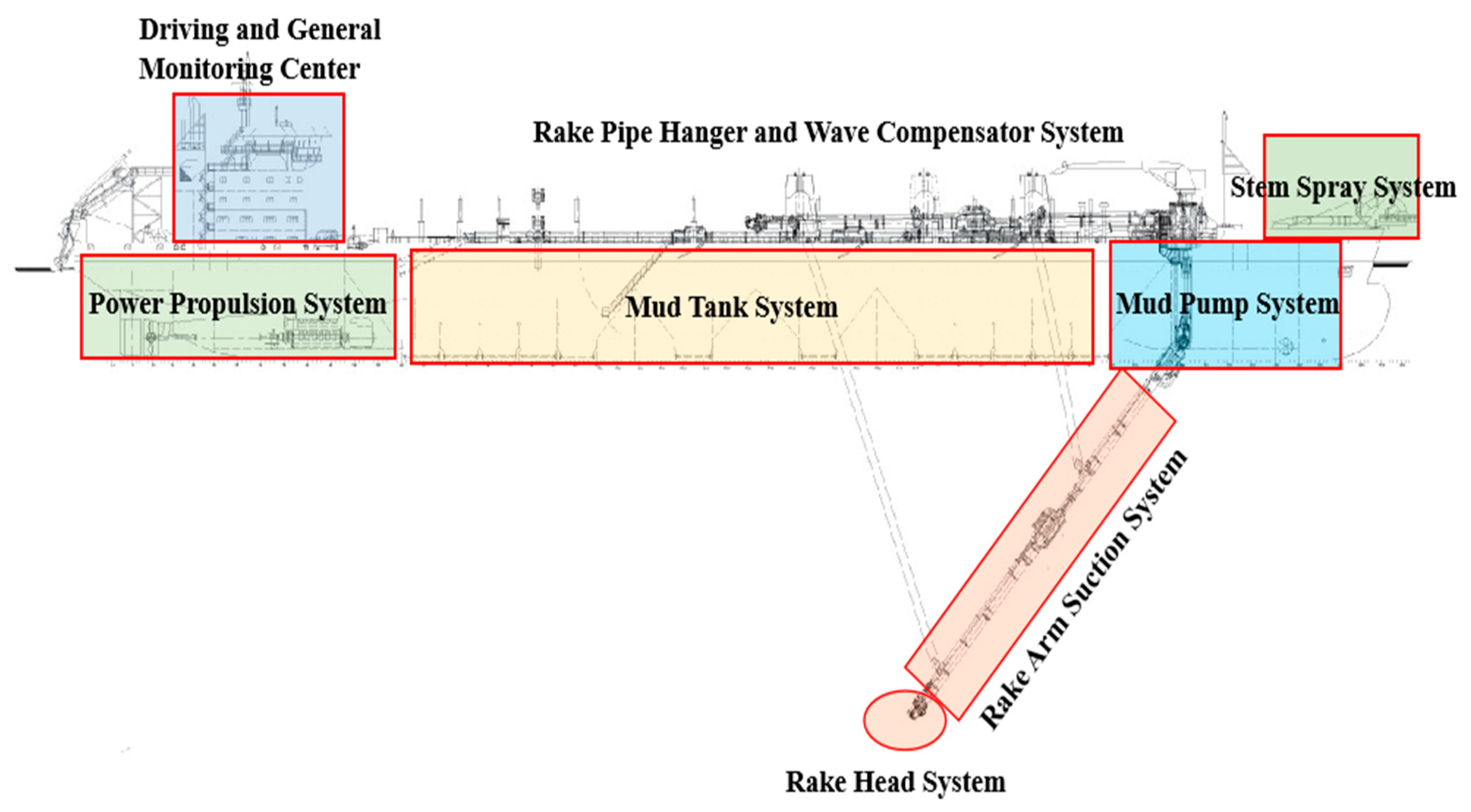
The TSHD collects dredged material through a rake arm, which is connected to a rake head similar to a vacuum cleaner, then sucks the dredged material from the bottom, and, finally, the dredged material is pumped to the hopper of the hull. Its basic structure is shown in Figure 1. The suction vessel sails from the dredging area to the dumping area when the hopper is full. Generally, the sediment in the mud hopper can be unloaded in three ways: it is unloaded through the bottom of the mud hopper, connected to the transmission pipeline, pumped to the mud-dumping area, and directly filled by ejection pipe. The TSHD can be self-digging, self-propelled, self-loading, self-unloading, self-blowing, etc., and has excellent navigation performance. It can carry out construction operations in the state of sailing and it does not need to occupy a large area or to block the channel during the construction process, thus it is especially suitable for construction in open harbors, long-distance channels in estuary areas, abysmal seas, etc.

2.2. Construction Method of TSHD

The method of the TSHD construction usually adopts the overflow-loading dredging method, and the efficiency of this construction method depends not only on the productivity of the tank but also on the length of the dredging cycle. Therefore, the overflow time of the TSHD cannot be simply measured by the maximum loading productivity, otherwise it may reduce productivity. When the ratio of the amount of earth onboard to the period reaches its maximum value, the amount of earth onboard per unit of time is the largest, i.e., the loading overflow time at this time is the best overflow time, that is to say, the shortest loading overflow time and the largest amount of loading ship. Conversely, the longer the loading overflow time, the fewer boats are loaded per unit of time. The optimal loading and overflow time is the loading and overflow time corresponding to the amount of earthwork carried when the product of the amount of earthwork onboard and the number of ships reaches the maximum in unit time. With the same cabin productivity and the same effective loading time, less overflow loss means higher loading efficiency and less energy waste. During construction, the TSHD digs trenches and puts the extracted mud into mud tanks. In the actual construction, the construction personnel need to adjust the overflow level according to the water depth, wind, and waves, the existing oil and water storage productivity in the ship, the soil quality, the actual effective load of sediment, etc., to determine the use of the tank productivity and to adapt to the possible allowable draft depth. This method of an operation mainly relies on experience to select appropriate parameters. Since the construction personnel mainly judge the current mining status according to the productivity index, the construction will be affected if the construction personnel cannot accurately predict the productivity within a reasonable time. Therefore, the problem studied in this paper is how to quickly and accurately predict the productivity of the dredger when the mud concentration meter is damaged, to assist the construction workers.

3. Methodology

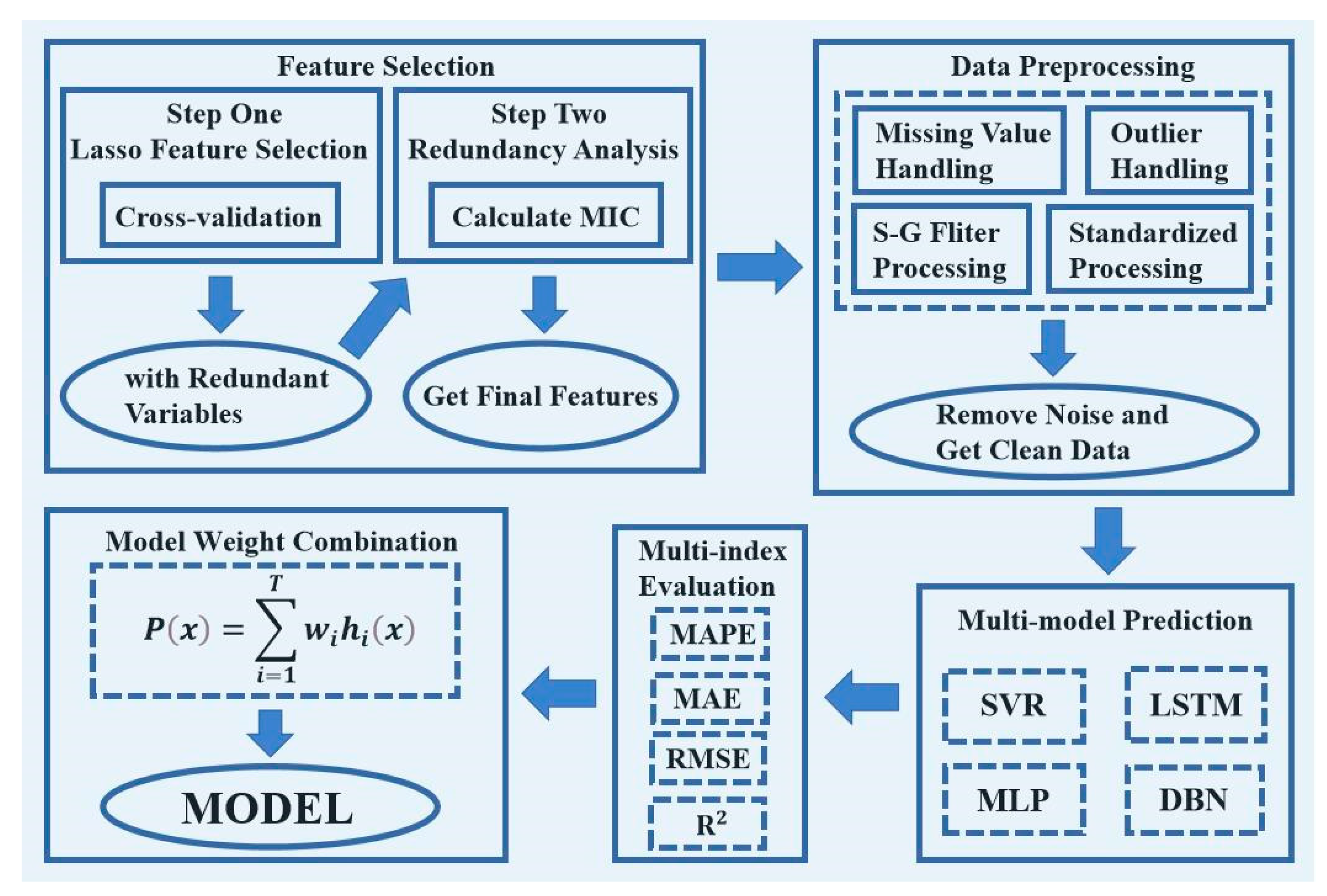
In this chapter, we propose a Lasso-MIC-based feature selection method and a weight combination model prediction method. Figure 2 shows the specific block diagram.

The research in this paper is mainly based on 316 sets of monitoring data collected by the data acquisition and monitoring control system (Supervisory Control and Data Acquisition, SCADA) of the TSHD, as shown in

Table 1. Monitoring data.

Order	1	2	3	4	5	6	……	315	316
(Point ID)	Sand Pump	Sand Pump Power	Host Power	Drag Angle	Discharge Pressure	Vacuum for Suction	……	Sand Pump Motor Speed	Drag Depth
	(Knot)	(KW)	(KW)	(°)	(Mpa)	(Mpa)		(r/min)	(m)
1	2.96	1084.11	5657	3.44	0.76	−0.81	……	974.85	20.78
2	2.91	1087.95	5625	3.42	0.76	−0.77	……	972.98	20.89
3	3.04	1084.35	5750	3.44	0.76	−0.76	……	967.85	20.68
4	3.03	1106.66	5794	3.53	0.76	−0.79	……	973.45	20.76
5	3.05	1092.65	5686	3.6	0.8	−0.78	……	974.38	20.81
6	3.03	1107.31	5587	3.56	0.77	−0.81	……	972.52	20.78
7	3.03	1116.7	5721	3.49	0.76	−0.82	……	973.45	20.63
8	3.07	1106.25	5651	3.51	0.71	−0.82	……	973.45	20.56
9	3.05	1109.8	5608	3.51	0.7	−0.81	……	974.38	20.59
10	2.98	1114.41	5657	3.66	0.73	−0.78	……	970.65	20.87
11	3.02	1132.62	5672	3.72	0.74	−0.79	……	972.52	20.66
12	2.99	1134.43	5672	3.9	0.74	−0.82	……	971.12	20.64
13	2.91	1118.99	5643	3.97	0.74	−0.81	……	975.32	20.81
14	3.01	1114.02	5602	3.94	0.74	−0.81	……	973.45	20.97
15	2.92	1141.98	5608	3.87	0.74	−0.83	……	973.45	20.91
16	2.88	1140.24	5855	3.93	0.78	−0.82	……	969.72	21.04
n	……	……	……	……	……	……	……	……	……

. First, we supplement the missing values in the original data with the interpolation method [17] and use the S-G filtering method to process data outliers [18]. Then, we use the Lasso model to perform the preliminary feature selection [19,20], and then the MIC algorithm removes redundant features [21] and obtains 12 feature variables with high correlation and low redundancy. After the prediction and fitting of models such as Support Vector Machine (SVR) and Deep Belief Nets (DBN), we compare the goodness of fit of each model, assign the best weight combination according to Formula (1), and combine them into a better strong learner to obtain the best-predicted value.

$$P(x)={{\displaystyle \sum }}_{i=1}^T{w}_i{h}_i(x)$$

(1)

where P(x) is the combined prediction result, i is the corresponding base learner category, T is the total number of base learners, w represents the weight of the base learner, and h(x) represents the base learner output.

3.1. Data Processing and Visualization

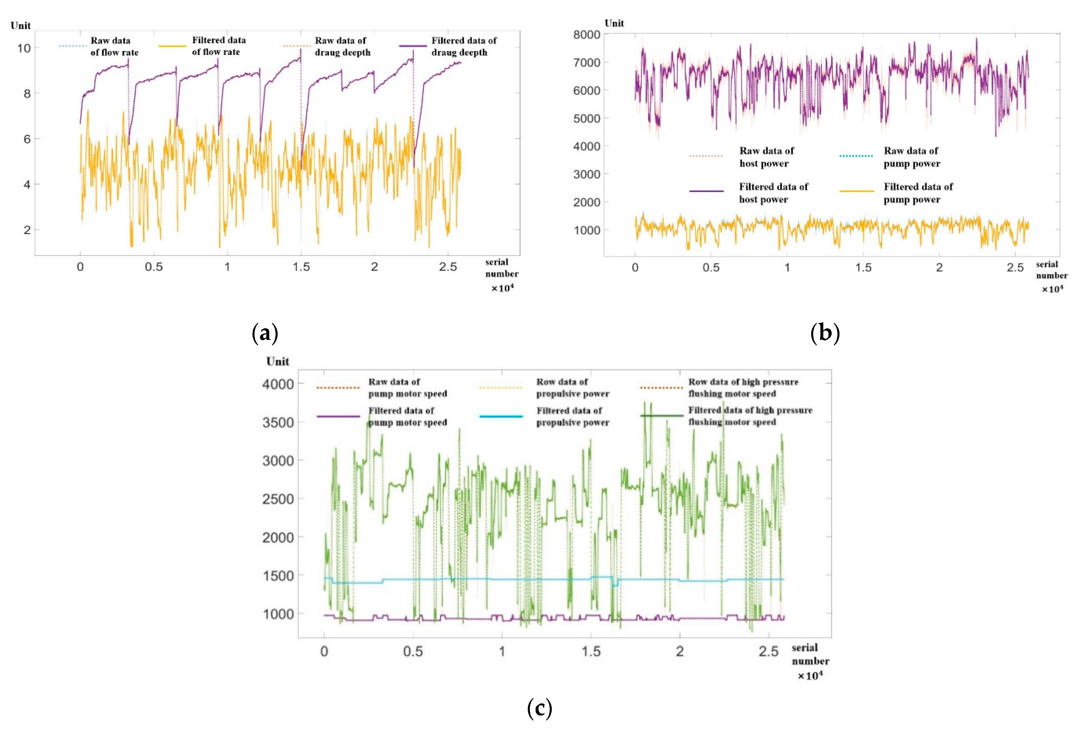
Due to a large number of missing values and outliers in the original data, data processing is required. Some of the missing data points are usually filled by interpolation algorithms, such as linear interpolation, nearest neighbor interpolation, etc. However, the processing of outliers has a greater impact on obtaining high-quality data, so we pay more attention to the processing of outliers.

Abnormal Data Processing

The S-G filter can be regarded as a filtering method based on local polynomial least squares fitting in the time domain, which has the advantage of keeping the shape and width of the sequence unchanged while filtering out noise. When a smoothing filter is used to filter a signal, the low-frequency components in the signal are fitted and the high-frequency components are smoothed out. If the noise is at a high frequency, the result of filtering is to remove the noise. On the contrary, if the noise is at a low frequency, the result of the filtering is to leave the noise. Using this method can improve the smoothness of the data and reduce the interference of the data noise. The filtered data are shown in Figure 3.

3.2. Feature Selection

Since the collected construction data contain useful and redundant monitoring data, if the data are directly input as modeling data, due to the high dimensionality of the data space, the huge amount of calculation and some variables will affect the prediction of the model precision. Therefore, feature selection must be done before modeling. Commonly used feature selection methods are filter, wrapper, embedding, etc. In the process of feature selection, the validity of feature variables and the elimination of redundancy between features should be taken into account. Similar to irrelevant features, redundant features also affect the speed and accuracy of model predictions and should be filtered. Based on this, we propose a feature selection method based on the Lasso and Maximum Information Coefficient (MIC).

The Lasso regression algorithm is a regression analysis method that performs feature selection and regularization at the same time. The principle of the algorithm is as follows: ordinary linear model.

$$Y=X\beta +\epsilon$$

(2)

The response variable $Y={\left(y_1,y_2,\dots ,y_n\right)}^T$, covariate $X=\left(X^{\left(1\right)},X^{\left(2\right)},\dots ,X^{\left(d\right)}\right)$. For each $X^{\left(j\right)}$, there is $X^{\left(j\right)}={\left(X_1^{\left(j\right)},X_2^{\left(j\right)},\dots ,X_n^{\left(j\right)}\right)}^T$. Assuming that each $X_i^{\left(j\right)}\left(i=1,2,\dots ,n,j=1,2,\dots ,d\right)$ is centered and normalized, the random error term ${\epsilon }_i=N\left(0,{\sigma }^2\right),\left(i=1,2,\dots ,n\right)$, $\epsilon ={\left({\epsilon }_1,{\epsilon }_2,\dots ,{\epsilon }_n\right)}^T$, regression coefficient $\beta ={\left({\beta }_1,{\beta }_2,\dots ,{\beta }_d\right)}^T$. When X is not a full-rank matrix, the ordinary least squares method will no longer be suitable for solving the regression coefficients and we introduce a penalty method at this time. The Lasso method is to add $l_1$ the penalty term to the ordinary linear model. This method can realize variable selection and parameter estimation at the same time. During parameter estimation, some parameters are compressed to zero to achieve the effect of variable selection. The penalty method is to take the value of the minimum penalty likelihood function as the estimated value of the regression coefficient, that is

$$\widehat{\beta }=arg min\left(Y-X{\beta }^2+P_{\lambda }\left(\left|\beta \right|\right)\right)$$

(3)

The penalty term $P_{\lambda }\left(\left|\beta \right|\right)=\lambda {\displaystyle {\displaystyle \sum }_{j=1}^d}{\left|{\beta }_j\right|}^m$, when m = 1, the $l_1$ penalty term is obtained. While fitting the data, Lasso also uses the $l_1$ norm to make the coefficients sparse to select features. For the ordinary linear model, Lasso is estimated as

$${\widehat{\beta }}_{Lasso}=arg min Y-X{\beta }^2 s.t.{{\displaystyle \sum }}_{j=1}^d\left|{\beta }_j\right|\le t,t\ge 0.$$

(4)

Equivalent to

$${\widehat{\beta }}_{Lasso}=arg min\left(Y-X{\beta }^2+\lambda {\displaystyle \sum }_{j=1}^d\left|{\beta }_j\right|\right)$$

(5)

In the above equation, n is the number of samples, d is the number of features, and m is the number of penalties, i.e., for m = 1, the $l_1$ penalty term is obtained (Lasso penalty); for m = 2, the $l_2$ penalty term is obtained (Ridge penalty).

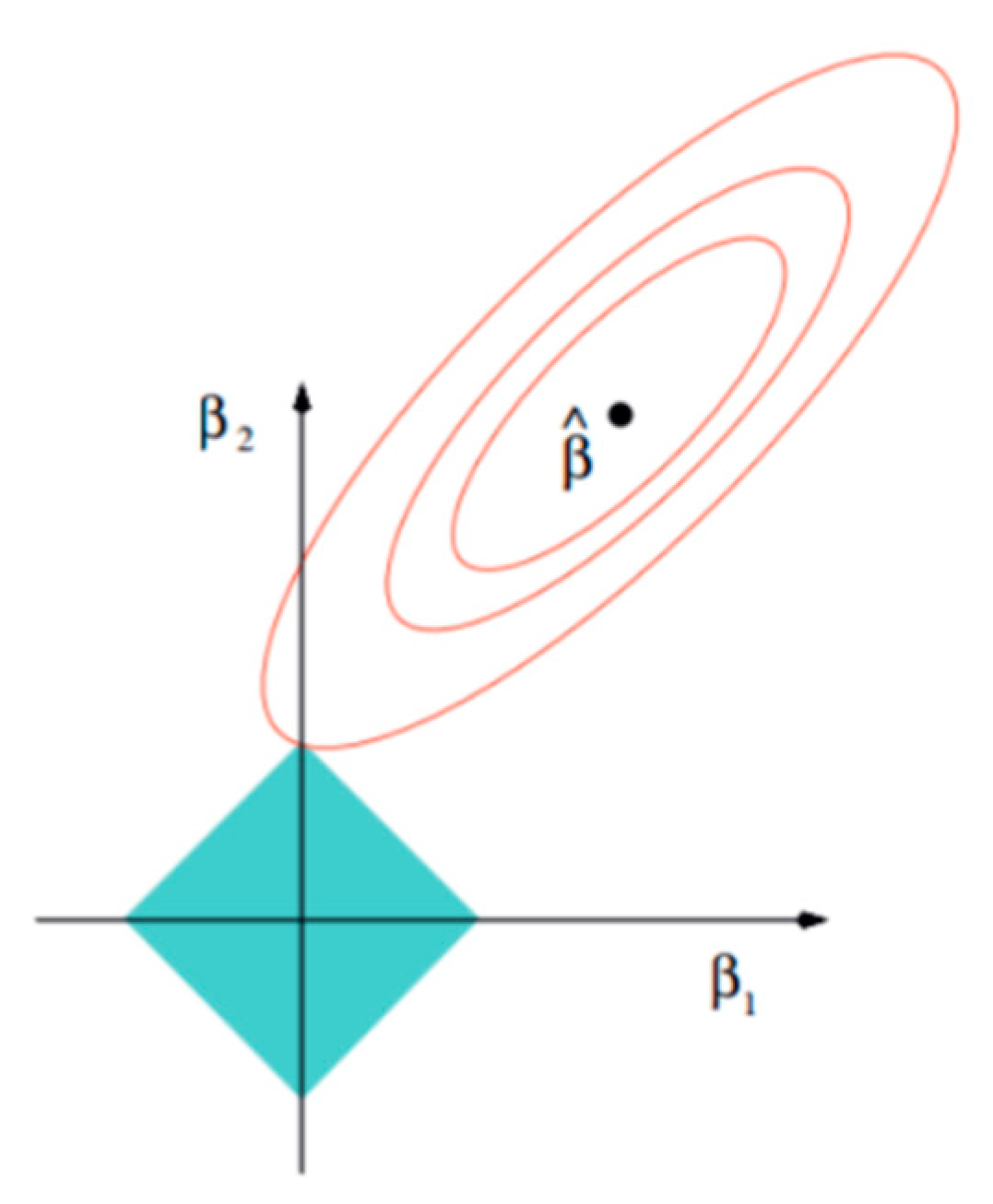
Among them, t and λ correspond one-to-one, which is the adjustment coefficient. Let $t_0={{\displaystyle \sum }}_{j=1}^d\left|{\widehat{\beta }}_j\left(OLS\right)\right|$, when t < $t_0$, part of the coefficients will be compressed to zero, thereby reducing the dimension of X and reducing the complexity of the model, so that the model has better interpretability.

For the above process, it is represented by a two-dimensional model space, as shown in Figure 4. That is, the model space is limited to an $l_1$− ball of w, the contour line of the objective function is made on the (w1, w2) plane, and the constraint condition is a norm ball with radius C on the plane. The optimal solution is where the contour first intersects the normal ball.

Compared with Pearson’s correlation coefficient method, Relief algorithm, chi-square test method, and other methods to eliminate feature redundancy, MIC can measure linear, nonlinear, non-functional relationships, and other dependencies. It can also mine more dependencies between categories and features. Through the above two methods, the characteristic variables that are effective for forecasting the production capacity of the trailing suction dredger are finally selected.

3.3. Model Fusion Prediction Algorithm

Support Vector Regression (SVR) is a branch of Support Vector Machine (SVM). Its learning strategy is to minimize the interval and finally convert it into a convex quadratic programming problem to obtain the global optimal solution and avoid the tendency to fall into local optimal [22]. A Deep Belief Network (DBN) is composed of multiple Restricted Boltzmann Machines (RBM) layers and is a typical grid structure [23]. These networks are “restricted” to a visible layer and a hidden layer, with connections between layers, but no connections between units within a layer. Hidden layer units are trained to capture higher-order data correlations represented in the visible layer. For this purpose, we set hidden units = (95,100), i.e., there are two hidden layers with 95 and 100 hidden units, respectively; we set batch size to 30, i.e., we crawl 30 data at a time; in addition, we set epoch pretrain = 60 and epoch finetune = 80 to improve computational efficiency and accuracy. Long Short-Term Memory (LSTM) is a special Recurrent Neural Network (RNN) structure with strong generalization and robustness. The LSTM unit consists of three multiplication gates. These “gates” control the retention and transmission of information. In addition, the storage unit of the LSTM controls access, writing, and clearing to prevent the gradient from disappearing too quickly [24]. In the process of using the LSTM model for prediction, we set the sequence length = 11, which means that when the LSTM processes the sequence data, the length of this sequence is 11. After repeated adjustments and trials, the best prediction result is obtained when the sequence length is 11. The essence of Multilayer Perceptron (MLP) is the extension and deepening of the linear model. Its algorithm is composed of a large number of simple neurons [25]. Each neuron accepts the input of a large number of other neurons. Through the nonlinear input and output relationship, the output affects other neurons. It can obtain the weight and structure of the network through training and learning, showing strong self-learning ability and adaptive ability to the environment. In this model, we set hidden layer_sizes = (128,32), i.e., there are two hidden layers with 128 and 32 neurons each, and set batch size = 32, i.e., 32 data are crawled at once; this combination predicts the best results.

3.4. Hyperparameter Optimization

Hyperparameter optimization in machine learning aims to find the hyperparameters that make machine learning algorithms perform best on validation datasets. Grid search is the simplest and most widely used hyperparameter search algorithm. We simply build independent models for all hyperparameter possibilities, evaluate the performance of each model, and choose the model and hyperparameters that yield the best results. Here, we use K-fold cross-validation, which divides the original data set into K equally, randomly takes out K-1 sample sets each time as the training set of the model, and the remaining sample set is used as the validation set of the model. Repeat the test K times, and finally average the results of the K times to generalize the error. This paper mainly uses the 10-fold cross-check method to find the optimal combination of the main parameters of each algorithm, and the optimal parameter combination is shown in the following table.

3.5. Error Metrics

To quantitatively evaluate the predictive performance of the model, error metrics are introduced in this paper. The significant values for each model prediction during the calculation are shown in

Table 2. Basic statistics.

	Minimum (m3/h)	Maximum (m3/h)	Average (m3/h)	Standard Deviation
SVR	2513.040	7472.422	5122.555	1274.228
LSTM	2465.210	7384.912	5052.289	1258.294
MLP	2271.430	7483.748	5064.945	1316.958
DBN	2469.946	7803.123	5206.234	1362.404
WCM	2336.883	7571.767	5118.075	1337.296

.

Error metrics are usually divided into longitudinal error and transverse error. Longitudinal errors are used to analyze the long-term operation of the system in amplitude, such as Mean Absolute Error (MAE), Mean Squared Error (RMSE), and Mean Absolute Percentage Error (MAPE). Use lateral error to study overall predictive performance, such as goodness of fit ($R^2$). The formula is as follows:

$$\{\begin{array}{c}MAE={{\displaystyle \sum }}_{i=1}^n\left|y_i-{\widehat{y}}_i\right|/n\\ RMSE=\sqrt{{{\displaystyle \sum }}_{i=1}^n{(y_i-{\widehat{y}}_i)}^2/n}\\ MAPE=\frac{1}{n}{{\displaystyle \sum }}_{i=1}^n\left|\frac{{\widehat{y}}_i-y_i}{y_i}\right|\\ R^2=1-{{\displaystyle \sum }}_{i=1}^n{(y_i-{\widehat{y}}_i)}^2/{{\displaystyle \sum }}_{i=1}^n{(y_i-\overline{y_i})}^2\end{array}$$

(6)

where n is the number of predicted values; ${\widehat{y}}_i$ is the predicted value; $y_i$ is the actual value.

4. Case Studies and Discussion

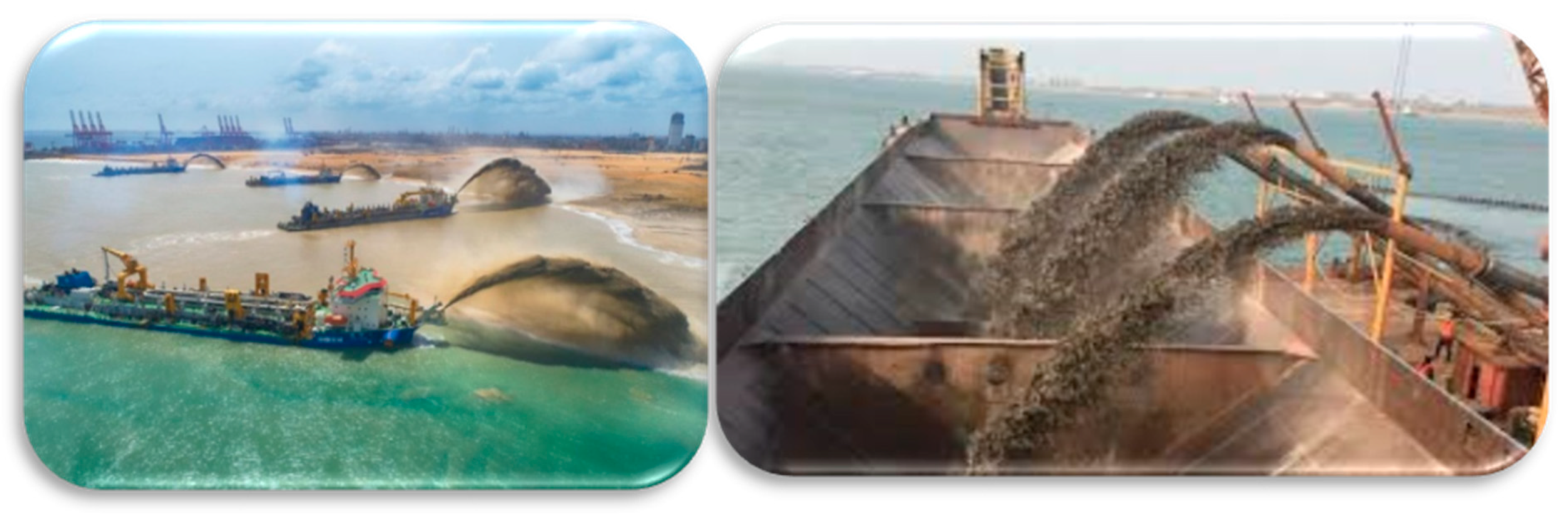
This study is based on the second phase of the 300,000-ton waterway project of Tianjin Port as the research background, the construction site is shown in Figure 5. The channel has a total length of 44 km and a total dredging volume of 13.5 million m³. After dredging, the effective channel bottom width can reach 397 m, the slope is 1:5, and the bottom elevation is −22 m. The main soil of the project includes silty clay, sandy silt, etc., and is mainly grade 6 dredged soil, which is hard in texture and difficult to excavate. The project was put into the construction of the “Tongtu” TSHD. During the construction process, the TSHD was in continuous operation. In this regard, SCADA recorded the data generated during construction and selected 14 cycles of construction operations of the towed suction dredger. The monitoring data from the non-overflow phase of the second dredging construction were used as a sample for the study, i.e., a 25,860 × 316 dimensional data matrix, and applied to subsequent machine learning processes such as dimensionality reduction as well as regression.

4.1. Data Preprocessing and Input Selection Analysis

Effective TSHD productivity predictions should be based on high-quality monitoring data. Therefore, the necessary data pre-processing needs to be carried out before modeling. As the generation of monitoring data is continuous during the actual dredging construction process, it is significantly time-dependent and continuous. As a result, anomalous values may be generated when there are sudden changes in influencing factors, such as dredging. Vessels sway substantially in wind and waves, and construction equipment or monitoring equipment malfunction. These outliers are generated independent of time, but they have the same temporal properties as normal data. It is therefore necessary to understand the time series of these anomalous data. In this paper, the S-G filtering algorithm is used to achieve the filtering of data noise, resulting in clean trending data.

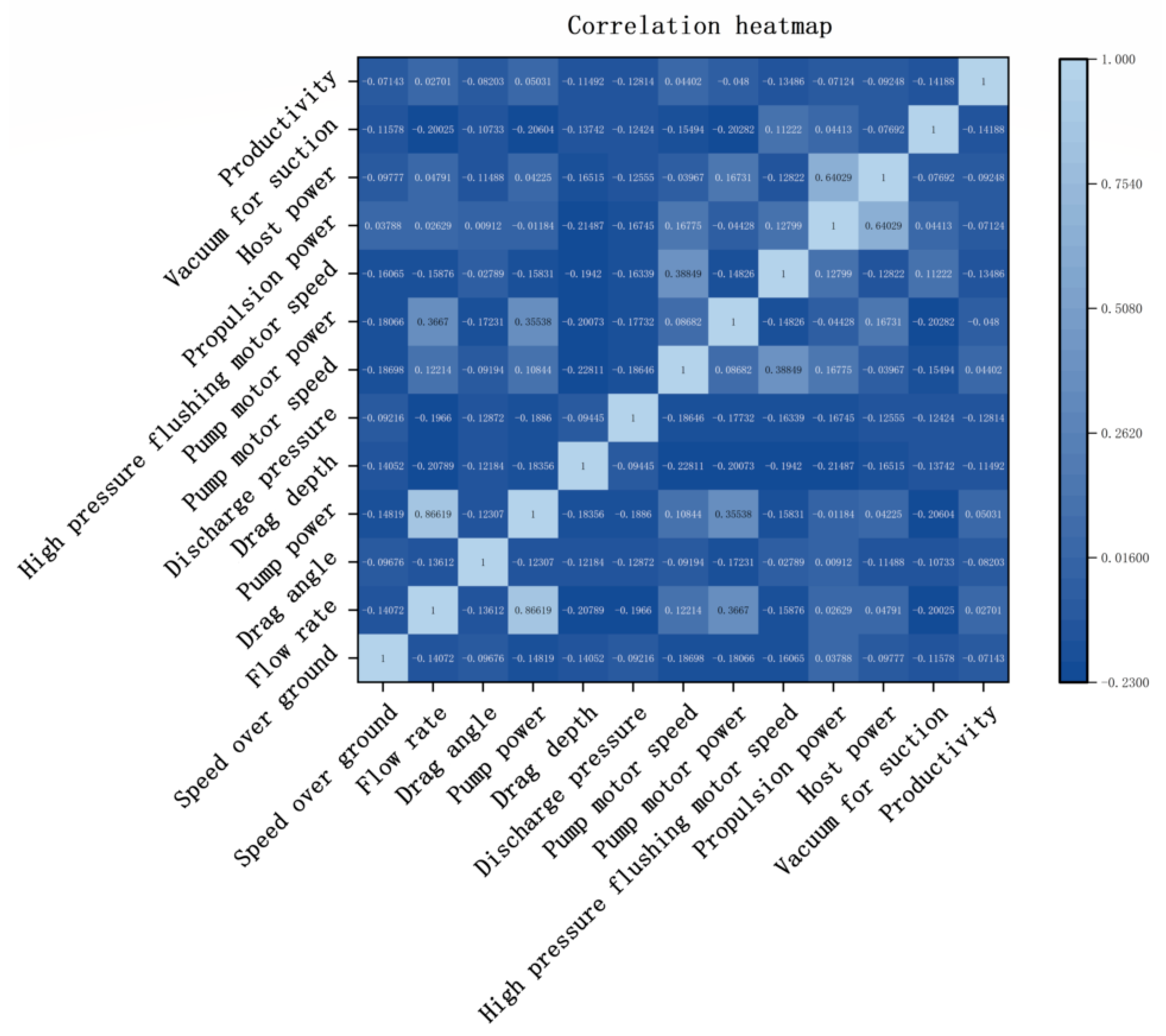
On the other hand, the towed dredger has up to 316 sets of monitoring data for five systems such as power system, vessel system, mud pump system, cabin system, and towing head systems, such as towing head angle, towing head depth, pump speed, and overland speed. We used the composite feature selection method above to initially filter out the feature variables affecting productivity using the Lasso model first to reduce the dimensionality of the data. This process, in addition to screening out features with high correlations with productivity, also requires the continuous removal of features with obvious mathematical relationships, thereby reducing the number of subsequent screenings. Even so, the high correlation between many variables still resulted in redundant characteristics. The 18 features initially screened by the Lasso model included “high-pressure flushing motor power” vs. “high-pressure flushing pump power” vs. “high-pressure flushing pump power” and “thrust” vs. “bow thrust”. The maximum mutual information coefficient between them is close to one and even reaches one, so here we continue to filter further using the MIC algorithm and these redundant features are removed to finally get 12 productivity-related features as shown in Figure 6. The contribution rates of these 12 features were obtained through the random forest, as shown in Figure 7, which also verified the reasonableness of the selected features.

4.2. Predictive Process Analysis

4.2.1. Data Normalization

In the process of data processing, we selected 24,000 sequence lengths as the training set and 646 sequence lengths as the test set after data preprocessing. Since the selected monitoring data belong to different categories, there is a dimension problem between the data, and the existence of the dimension will affect the final modeling result. Therefore, we choose to use Z-Score normalization to convert these data of different dimensions into a unified measure, which speeds up the gradient descent and improves the comparability of the data. Its formula is:

$$x_{norm}=\frac{x-\mu }{\sigma }$$

(7)

where μ and σ are the mean and standard deviation of the original data, respectively.

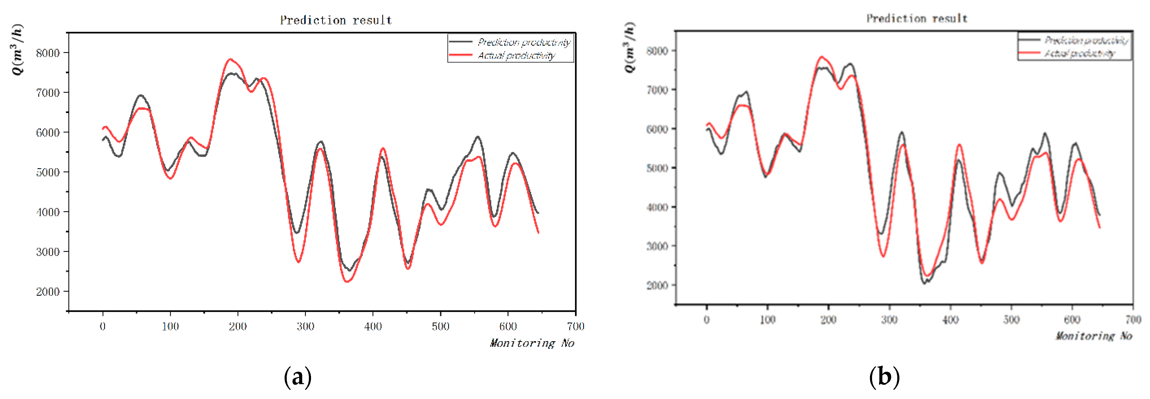
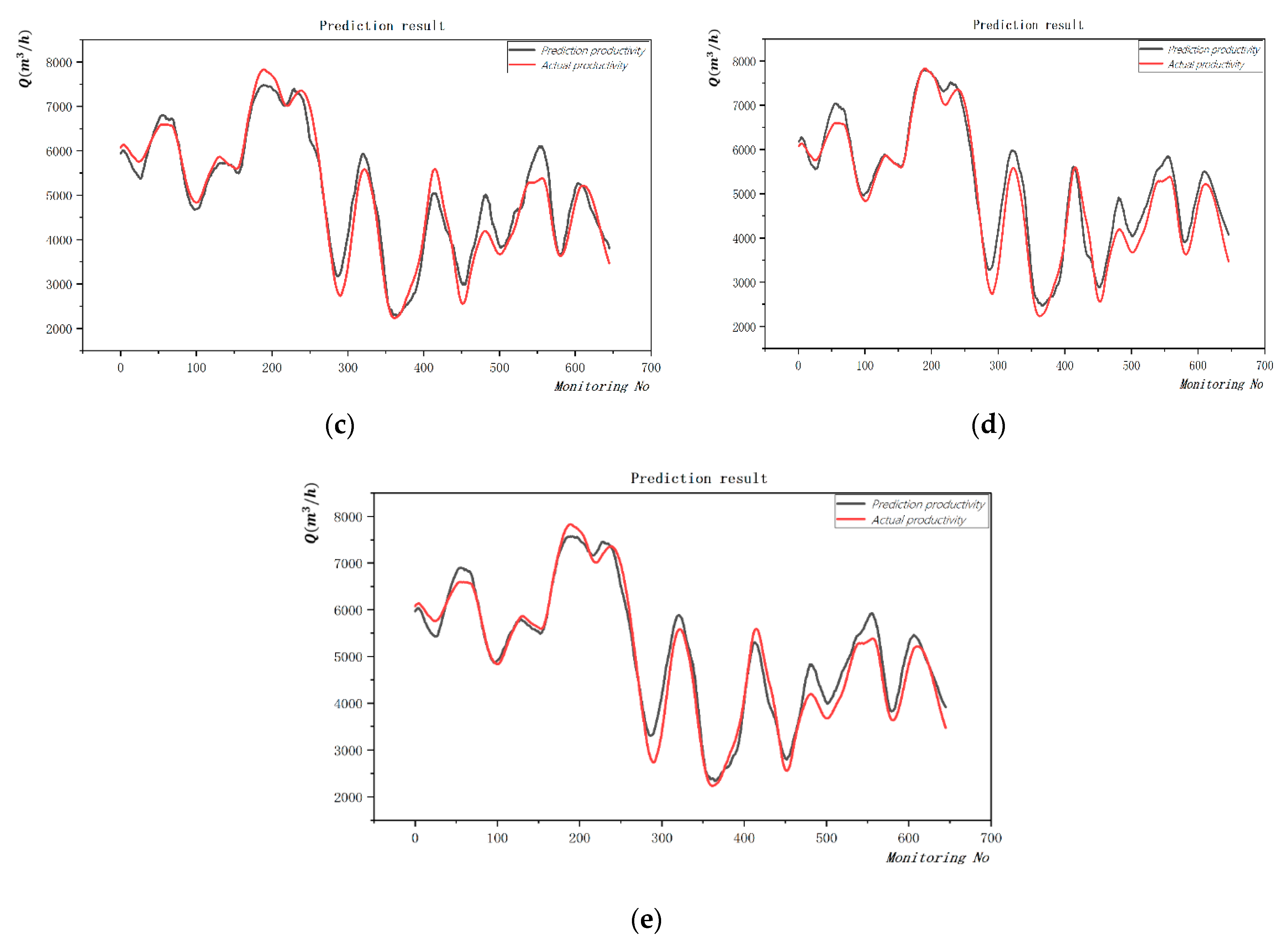
4.2.2. Prediction Analysis of Each Model and Weight Model

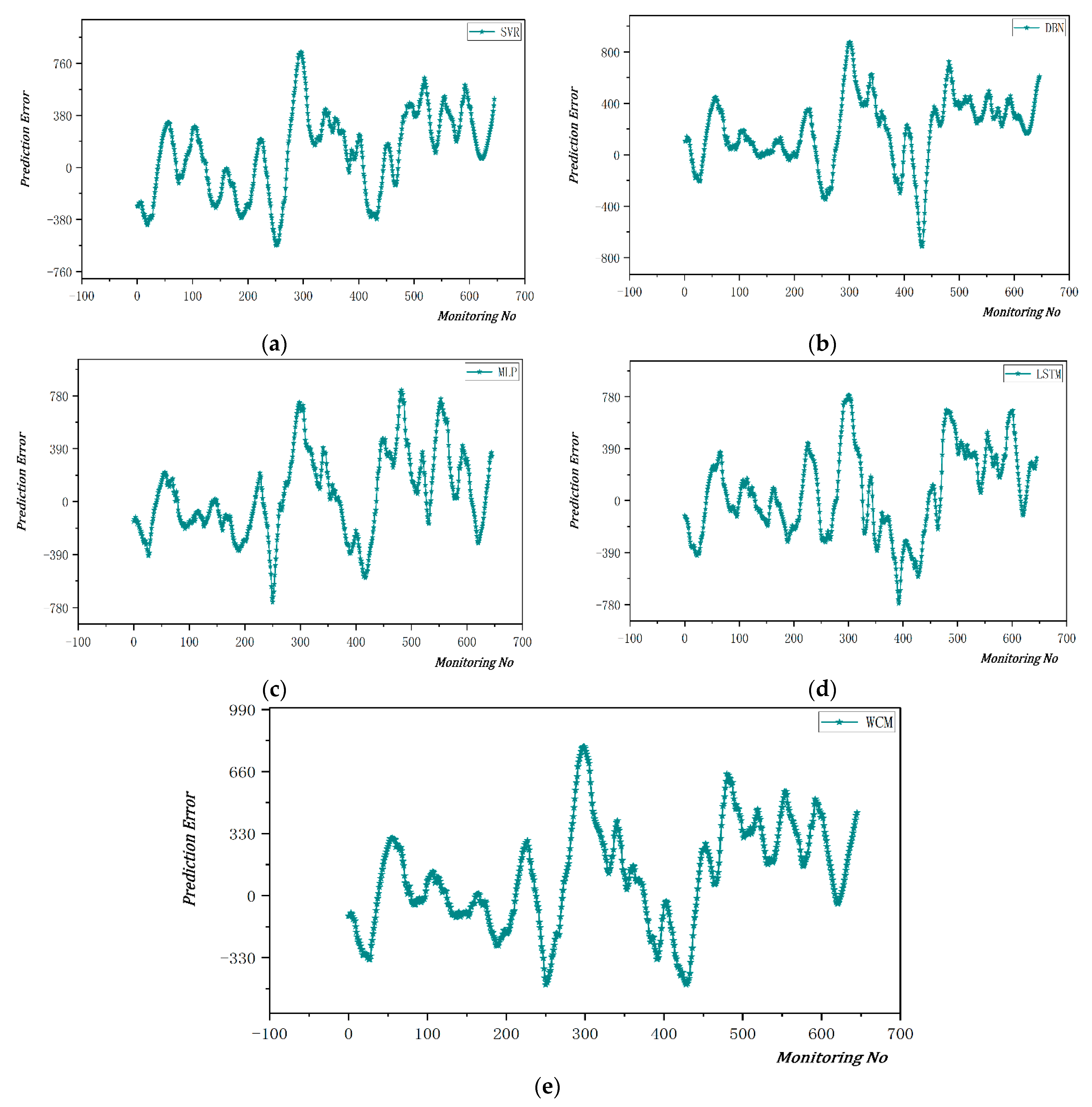
To optimize the algorithm performance of the weight model, it is necessary to carry out research and analysis based on the learning ability of each model. First of all, it can be seen from the Figure 8 that each model has different prediction errors at the same position, indicating that these models have complementary advantages. From the prediction of $R^2$, the prediction effect of deep learning MLP is the best, reaching 0.9517, and MLP is also the best in terms of mean error (MAE), mean absolute percentage error (MAPE), and mean square error (RMSE). An artificial intelligence algorithm is to find the mathematical relationship between input and output, and its core is model, algorithm, and strategy. For the model, most problems are still solved by a single model. Due to the large hypothesis space of the operation data of the TSHD, there may be multiple hypotheses that can achieve the same prediction effect during training. At this time, if a single model is used, which may cause poor generalization performance of the model due to randomness, the algorithm is an optimization solution to the model, and the strategy is a combination of the model here. Based on considering the prediction information of multiple prediction models, evaluate the prediction results, use the percentage of the prediction accuracy to the prediction accuracy of the overall model as the weight of the combination strategy, and use Formula (1) to weight the results.

Among them, P(x) is the combined prediction result, I is the corresponding basic learner category, T is the total number of basic learners, ω represents the weight of the basic learner, and h(x) represents the output of the basic learner. Among the four algorithms mentioned above, the optimal hyperparameter set obtained after the parameter adjustment of a single model is shown in

Table 3. Super parameters and evaluation indexes of each algorithm.

Algorithm Name	Hyper Parameter Set	Model Predict Index
		RMSE	MAE	MAPE	R2
LSTM	learning_rate = 0.016; decay1 = 0.0001; beta_1 = 0.96; beta_2 = 0.997; 1r = 0.003	328.68	269.95	0.062	0.9462
DBN	epoch_pretrain = 40; epoch_finetune = 80; batch_size = 31; hidden_units = (95,100)	328.29	268.29	0.058	0.9463
MLP	alpha = 0.001; batch_size = 33; max_iter = 500; learning_rate_init = 0.005; random_state = 1	311.33	249.82	0.053	0.9517
SVR	degree = 3; gamma = 0.01; coef0 = 0.6; tol = 0.001; C = 6; max_iter = −1; epsilon = 0.3	315.99	267.89	0.057	0.9503
WCM	SVR = 0.2504; MLP = 0.2508; LSTM = 0.2494; DBN = 0.2494	290.59	235.39	0.050	0.9528

below, and the prediction results of each model are shown in the following figure.

According to the weight combination formula, the combined weight is allocated according to the goodness of fit ($R^2$) predicted by each model. The final weight allocation of SVR, MLP, LSTM, and DBN is 0.2504, 0.2508, 0.2494, and 0.2494, respectively.

Given the limitations and contingency of a single model, the prediction results should be deeply fused. In layman’s terms, “learning” in machine learning means continuous “training” through massive data, essentially changing the corresponding “weight”. Here, the model itself is jumped out, and the corresponding weight strategy allocation is made between different models. In the whole process, it not only analyzes the prediction effect of a single base learner but also comprehensively compares the combined effect of each base learner, making the overall model obtain the best effect.

Compared with a single model, the ensemble model after weight combination gives full play to the advantages of each model, on the one hand, neutralizing the part that the prediction results of different models do not fit well, and at the same time, reducing the problem that a single model may perform poorly on unknown test data. On the other hand, during the training process of a single model, the model often has the risk of falling into a local minimum point, and the possible result is that the trained model only fits the current test data well and cannot predict unknown data. However, after running multiple learners and combining weights, the influence of local minima can be effectively reduced. Figure 9 visualizes the prediction error analysis for each model.

5. Discussion

The extensive use of the TSHD to a certain extent meets the needs of our country for building deep-water ports and sea reclamation, but dredging engineering construction is a complex and non-constant dynamic process; the adjustment of parameters in the construction process is directly related to the dredging efficiency and the construction cost of TSHD and has an important impact on the safe operation of the dredging equipment. Therefore, it is necessary to analyze and optimize the construction capacity of the TSHD. In this study, we carried out feature selection, data preprocessing, and model prediction for the construction data of large-scale TSHD in the Tianjin port channel dredging project, and then assigned weights according to the goodness of fit predicted by each model and obtained a new weight combination model; it is found that its optimization effect is obvious after comparing multiple error metrics. The method greatly improves the productivity of the TSHD and has important economic and social benefits. Compared with previous studies, the characteristics of this study are as follows:

(1)

In terms of feature selection, we propose a novel feature selection method to select the best key indicator parameters, which is based on the Lasso and Maximum Information Coefficient (MIC) redundant identification. This method may not only take into account the correlation between features and categories but can also filter out the redundancy between features, which ensures the speed and accuracy of machine learning so that we can finally get a high correlation and low redundancy feature subset.

(2)

In terms of data preprocessing, we conduct an in-depth analysis of the data structure of the TSHD and propose solutions for data preprocessing, including missing value processing, outlier processing, S-G filtering processing, and standardization processing. The S-G filter can be regarded as a filtering method based on local polynomial least squares fitting in the time domain. Its advantage is that it can keep the shape and width of the sequence unchanged while removing noise, so that the final obtained data are relatively clean and have less impact on the original data, which provides data quality assurance for subsequent capacity optimization analysis.

(3)

In terms of research characteristics, this paper studies and analyzes the learning ability of each model, and proposes that they can be recombined according to the different weights of each model to obtain an integrated model that can achieve full use of the advantages of a single model and finally obtain better predictions’ effect. The method well meets the demand for intelligent dredgers for large projects, further improves the real-time monitoring system, and also plays a positive role in improving the real-time dredging output of the TSHD, optimizing construction control, reducing production costs, and detecting equipment abnormalities in advance.

6. Conclusions

This paper draws on cutting-edge algorithm technology in the field of artificial intelligence and machine learning. The feature selection method based on Lasso–MIC and the prediction algorithm of the weight combination model are proposed and applied to the productivity prediction of the TSHD. The specific conclusions are as follows:

(1)

It is proposed to use the Lasso model and the MIC model comprehensively to screen out feature combinations with high correlation and low redundancy and to use S-G filtering and standardization methods to preprocess data, which improves the quality of related data.

(2)

By analyzing the prediction results of each model, comparing the size of $R^2$ of each model, calculating the corresponding weight according to the formula, and constructing a weight combination model, this further improves the accuracy of the prediction. The research proves that the method has broad application prospects, can accurately predict the productivity of the TSHD, and can improve its operational efficiency of it.

(3)

By using machine learning algorithms to mine and analyze historical data, modeling of the production process can be omitted. The method improves prediction accuracy, reduces the limitation of remote management of dredging work, increases the number of controllable operations, and actively changes the dredging work from onsite personnel inspection to data log system management, which improves the intelligence of dredging work.

The conventional diagnostic methods currently in use on rake suction vessels are still at a relatively outdated stage, such as broken wire checks and signal range checks. For example, the system alerts when the measured value of a pressure sensor is above or below a set threshold, but with the help of computer simulation technology, it is possible to diagnose the system of a rake suction vessel directly and detect more complex and interactive system deviations. As the concentration sensors are subject to long periods of operation such as operating temperature, humidity, and tube wall adhesion, the predictive simulation method described above enables small deviations from the concentration sensors to be detected, and when the concentration sensors are temporarily out of order or damaged, the simulated values from the algorithm described above can be used to display them instead. The method thus aims to maintain the reliability of the concentration signal (productivity signal) in the rake suction vessel system by predicting real-time productivity. In practice, it provides real-time and reliable productivity information for the operator or the automatic control system, ensuring that the performance of the TSHD is optimized and improved, increasing the uptime.

Based on the research in this paper, in-depth research and analysis can be done in the following several aspects in the future.

Limited by the time, data, and technical limitations of the research, this paper only proposes a productivity prediction model based on productivity. Hundreds of monitoring instruments on the TSHD are gradually optimized. These monitoring data quantitatively reflect the relationship between production capacity, operation, and other equipment parameters to a certain extent, and are also of great significance for improving productivity and reducing construction costs.

There is no real-time one-to-one correspondence between the input factors and the output factors of the productivity prediction of the TSHD, and the correspondence between them is complicated. In the actual dredging process, most of the real-time parameters in the construction process are collected by instruments. However, the density meter of the TSHD is installed at the outlet of the mud pump pipeline, which is separated from the rake head that sucks the soil in real time. It is not installed in the same position as the concentration meter that measures the mud concentration, which means that there is a position difference between these instruments, which leads to the occurrence of time lag problems. Therefore, the output control of the TSHD has the characteristics of large time delay, uncertainty, and temporal variability, and the removal of time lag should be considered to better carry out mathematical modeling.

At present, most of the optimized operation of the raking suction ship still relies on the raker operator. However, since the working conditions will continue to change during the dredging construction process, the difficulty of the raker operator adjusting various parameters will also increase accordingly, which increases the staff’s difficulty. The workload and ease cause the phenomenon of low control accuracy. Therefore, it should be considered to further develop the dredging intelligent operation system, improve the intelligence level of the dredging industry, reduce the influence of human and subjective factors on construction, and also reduce labor costs.

In addition to the equipment capacity of the dredging, soil quality is also a key factor affecting the productivity of the TSHD. Most of the current dredging operations use borehole sampling to describe the soil quality of the dredged area. There are two problems with this method: First, the cost of drilling borehole sampling in the ocean is extremely high. Second, it is difficult to cover the entire area with limited borehole samples, and the accuracy of the soil model is still poor and cannot achieve the purpose of predicting relevant parameters. In the future, through a large amount of construction data, artificial intelligence can be used to predict soil parameters in real-time in combination with ship operating parameters, and the construction parameters of the dredger can be adjusted accordingly to further optimize construction efficiency.

References

- Chou, J.S.; Chiu, Y.C. Identifying critical risk factors and responses of river dredging projects for knowledge management within organization. J. Flood Risk Manag. 2021, 14, e12690. [Google Scholar] [CrossRef]
- Skibniewski, M.J.; Vecino, G.A. Web-based project management framework for dredging projects. J. Manag. Eng. 2012, 28, 127–139. [Google Scholar] [CrossRef]
- Chaudhuri, B.; Ghosh, A.; Yadav, B.; Dubey, R.P.; Samadder, P.; Ghosh, A.; Das, S.; Majumder, S.; Bhandari, S.; Singh, N.; et al. Evaluation of dredging efficiency indices of TSHDs deployed in a navigational channel leading to Haldia Dock Complex. ISH J. Hydraul. Eng. 2022, 28 (Suppl. S1), 471–479. [Google Scholar] [CrossRef]
- Bai, S.; Li, M.; Lu, Q.; Tian, H.; Qin, L. Global time optimization method for dredging construction cycles of trailing suction hopper dredger based on Grey System Model. J. Constr. Eng. Manag. 2022, 148, 04021198. [Google Scholar] [CrossRef]
- Li, M.; Lu, Q.; Bai, S.; Zhang, M.; Tian, H.; Qin, L. Digital twin-driven virtual sensor approach for safe construction operations of trailing suction hopper dredger. Autom. Constr. 2021, 132, 103961. [Google Scholar] [CrossRef]
- Wang, B.; Fan, S.; Jiang, P.; Xing, T.; Fang, Z.; Wen, Q. Research on predicting the productivity of cutter suction dredgers based on data mining with model stacked generalization. Ocean Eng. 2020, 217, 108001. [Google Scholar] [CrossRef]
- Wei, C.; Wei, Y.; Ji, Z. Model predictive control for slurry pipeline transportation of a cutter suction dredger. Ocean Eng. 2021, 227, 108893. [Google Scholar] [CrossRef]
- Park, J.; Kim, K.; Cho, Y.K. Framework of automated construction-safety monitoring using cloud-enabled BIM and BLE mobile tracking sensors. J. Constr. Eng. Manag. 2017, 143, 05016019. [Google Scholar] [CrossRef]
- Tang, J.Z.; Wang, Q.F. Online fault diagnosis and prevention expert system for dredgers. Expert Syst. Appl. 2008, 34, 511–521. [Google Scholar] [CrossRef]
- Tang, J.Z.; Wang, Q.F.; Bi, Z.Y. Expert system for operation optimization and control of cutter suction dredger. Expert Syst. Appl. 2008, 34, 2180–2192. [Google Scholar] [CrossRef]
- Bai, S.; Li, M.; Song, L.; Ren, Q.; Qin, L.; Fu, J. Productivity analysis of trailing suction hopper dredgers using stacking strategy. Autom. Constr. 2021, 122, 103470. [Google Scholar] [CrossRef]
- Bai, S.; Li, M.; Kong, R.; Han, S.; Li, H.; Qin, L. Data mining approach to construction productivity prediction for cutter suction dredgers. Automat. Constr. 2019, 105, 102833. [Google Scholar] [CrossRef]
- Tang, J.; Wang, Q.; Zhong, T. Automatic monitoring and control of cutter suction dredger. Automat. Constr. 2009, 18, 194–203. [Google Scholar] [CrossRef]
- Chen, X.; Miedema, S.A.; Van Rhee, C. Numerical modeling of excavation process in dredging engineering. Procedia Eng. 2015, 102, 804–814. [Google Scholar] [CrossRef]
- Li, M.; Kong, R.; Han, S.; Tian, G.; Qin, L. Novel method of construction-efficiency evaluation of cutter suction dredger based on real-time monitoring data. J. Waterw. Port Coast. Ocean Eng. 2018, 144, 05018007. [Google Scholar] [CrossRef]
- Yue, P.; Zhong, D.; Miao, Z.; Yu, J. Prediction of dredging productivity using a rock and soil classification model. J. Waterw. Port Coast. Ocean Eng. 2015, 141, 06015001. [Google Scholar] [CrossRef]
- García, S.; Luengo, J.; Herrera, F. Tutorial on practical tips of the most influential data preprocessing algorithms in data mining. Knowl.-Based Syst. 2016, 98, 1–29. [Google Scholar] [CrossRef]
- García, S.; Ramírez-Gallego, S.; Luengo, J.; Benítez, J.M.; Herrera, F. Big data preprocessing: Methods and prospects. Big Data Anal. 2016, 1, 9. [Google Scholar] [CrossRef]
- Liu, H.; Yu, L. Toward integrating feature selection algorithms for classification and clustering. IEEE Trans. Knowl. Data Eng. 2005, 17, 491–502. [Google Scholar]
- Cai, J.; Luo, J.; Wang, S.; Yang, S. Feature selection in machine learning: A new perspective. Neurocomputing 2018, 300, 70–79. [Google Scholar] [CrossRef]
- Zhou, H.; Zhang, Y.; Zhang, Y.; Liu, H. Feature selection based on conditional mutual information: Minimum conditional relevance and minimum conditional redundancy. Appl. Intell. 2019, 49, 883–896. [Google Scholar] [CrossRef]
- Balogun, A.L.; Rezaie, F.; Pham, Q.B.; Gigović, L.; Drobnjak, S.; Aina, Y.A.; Panahi, M.; Yekeen, S.T.; Lee, S. Spatial prediction of landslide susceptibility in western Serbia using hybrid support vector regression (SVR) with GWO, BAT and COA algorithms. Geosci. Front. 2021, 12, 101104. [Google Scholar] [CrossRef]
- Chen, A.; Fu, Y.; Zheng, X.; Lu, G. An efficient network behavior anomaly detection using a hybrid DBN-LSTM network. Comput. Secur. 2022, 114, 102600. [Google Scholar] [CrossRef]
- Yu, Y.; Si, X.; Hu, C.; Zhang, J. A review of recurrent neural networks: LSTM cells and network architectures. Neural Comput. 2019, 31, 1235–1270. [Google Scholar] [CrossRef] [PubMed]
- Desai, M.; Shah, M. An anatomization on breast cancer detection and diagnosis employing multi-layer perceptron neural network (MLP) and Convolutional neural network (CNN). Clin. eHealth 2021, 4, 1–11. [Google Scholar] [CrossRef]