Abstract
In seismic risk estimation, among the different types of fragility curves used (judgement-based, mechanical, empirical/observational, hybrid), the mechanical ones have the twofold advantage of allowing a better control over the basic parameters and of representing a validation test of the consistency of empirical/observational ones. In this study, fragility curves of RC frames with column-driven failures are obtained from a simplified analytical pushover method implemented in a simple spreadsheet, thus allowing the user to perform a large number of analyses. More importantly, the proposed method introduces the concept that Limit States at the structural level are obtained consequent to the attainment of the same Limit States at the local level, in the columns’ sections. This avoids using additional criteria, such as interstorey drift thresholds. This simple analytical model allows for rapid development of fragility curves, for any Limit State, of different building typologies identified by a set of global quantities (number of storeys, story heights, number of spans and span lengths) and by a set of local quantities (element sizes, reinforcement, and material properties). It also allows for a straightforward treatment of the influence of the soil class on the fragility curves parameters, which is another critical issue addressed in this work that helps when interpreting some literature results using empirical/observational methods.
1. Introduction
In the recent past, the topic of seismic risk analysis and mitigation has attracted the research community worldwide. Large-scale territorial studies have emphasized the need for developing risk analysis tools to be utilized by both civil protection agencies and insurance companies [1,2]. One of the main components of seismic risk is the vulnerability of structures. Dunand and Guneguen [3] showed that, even in regions with moderate seismic hazard, a high seismic risk can be found if the seismic vulnerability of the construction stock is high.
A convenient and widely adopted method for defining seismic vulnerability is the use of Fragility Curves (FCs). Such curves provide the probability of exceeding a Limit State (LS) or a Damage Level (DL) as function of a seismic intensity measure.
Different classifications have been proposed of the methods adopted to derive FCs [4,5]. A meaningful classification identifies four different groups of procedures, based on the main source of information: (a) judgement-based, (b) mechanical, (c) empirical/observational, and (d) hybrid.
Judgement-based FCs are derived from statistical treatment of estimates provided by experts about the average DL that various types of structures may undergo when subjected to different levels of seismic motion. The main advantage of this method is that it cannot be affected by shortage of data because experts can be asked to provide estimates for any structural type and ground motion severity. However, these FCs seem too subjective and may be biased by possible cross-influence among experts.
Mechanical methods, on the other hand, derive FCs from statistical elaboration of the results of analytical/mechanical models [6]. The assessment of buildings in mechanical methods for deriving FCs can be carried out through either: (a) non-linear dynamic analysis [7,8] or (b) simplified pushover analysis. In the literature, several simplified methods for the assessment of buildings are developed [9,10,11]. Expeditious pushover methods enable conducting analysis on a large scale, but their simplified formulation is often affected by certain drawbacks and limitations. The reliability of the so-obtained FCs strongly depends on the representativeness of the adopted model with respect to the structural typology it represents. When dealing with structural typologies, less care of details is required, since the range of variation of typological quantities is usually large. Refined models, apart from being computationally expensive in large-scale vulnerability analyses, would lack the knowledge of several input parameters. Thus, simple models, even 2D, as those dealt with in this work, are more effective, especially in view of territorial studies where relative rather than absolute risk of different building typologies is sought.
Empirical/observational methods are based on the statistical treatment of data collected in post-earthquake surveys [12,13,14,15]. The main advantage of these methods consists of the employment of the most realistic sources of information as to building features, damage pattern, ground motion, site effects, source, and path of the seismic waves, and so on. However, very rarely are these data disaggregated, so that databases eventually contain heterogeneous data referring to buildings: (1) built with different local construction practices, (2) built on different soil categories, and (3) surveyed by different technicians in different times and with different forms. Homogeneous datasets, on the other hand, may present low statistical significance.
Hybrid methods tend to overcome the limits of each of the other procedures by statistically elaborating a combination of different sources of information, as the method proposed by Kappos et al. [16], which combines empirical data and analytical results.
Overall, with respect to other methods, mechanical methods allow disaggregating large building stocks in more detailed subsets, and also allowing including the effects of different soil categories, so to perform more meaningful risk studies. Such features render this method ideal for use in parametric studies for the definition and calibration of territorial policies relevant to urban planning, retrofitting, insurance, and others.
The main objective of this study is to highlight the influence of local site characteristics, such as soil class and location, over the development of FCs. For this purpose, a simplified mechanical model for the assessment of RC frames is developed, which enables conducting analysis on a large scale with affordable computational effort. Finally, the resulting FCs in this study are compared to some observational and analytical FCs available in the literature. The study shows that local hazard and local soil class significantly affect the resulting FCs. Consequently, FCs pertaining to the same typology/building change when used at different locations and on different soil classes.
2. Determination of Displacement Capacity of 2D Frame
2.1. Simplified Analytical Model of A 2D Frame
To describe the global geometry of a 2D frame, representative of a building typology, only a small yet significant set of parameters is needed, such as: number of storeys, storey heights, number of spans, and span lengths. Permanent and variable loads are generally known from the building category. As far as materials are concerned, they can be deduced from the codes enforced at the time of construction of the building. The same codes can be used to deduce the element sizes and the amount of longitudinal and transverse reinforcement, either using the minimum amounts thereby defined or through a simulated design according to the then-enforced rules.
The simplified analytical model of a 2D frame rests on its interpretation as a series system of storeys, which in turn are considered as parallel systems of columns, which in turn are considered as series systems of flexural and shear-resisting mechanisms. Notwithstanding the simplified system logic, such models represent a reasonable compromise between typological representativeness and computational efficiency. The method is conceived to be applied to existing buildings designed for gravity loads, where failures are generally column-driven, since columns are often weaker than the framing beams. Additionally, due consideration is given to failure of beam-column joints by limiting the capacity of the framing columns accordingly.
One main issue arising when developing mechanical FCs is the global Damage Levels (DL) definition. Here, some correspondence is established with the analytically defined local Limit States (LS) at both the sectional and the element level. This step is essential in that DLs, which have been defined mainly to facilitate and homogenize observational data, are usually given in descriptive terms and, as such, suffer from being qualitative and subjective. On the other hand, LSs are quantitively and objectively stated and are therefore analytically usable.
In this study, the 2D frame response at the global level is described in terms of base-shear vs. top-displacement by a piece-wise trilinear curve, where three objectively measured LSs are identified: Damage limitation Limit State (DLS), Life safety Limit State (LLS) and Collapse prevention Limit State (CLS).
These three global LSs are directly obtained from the corresponding LSs of each single story, which in turn are derived from the LSs of each single column, which, again, are derived from the local LSs of the sections at the column’s end plastic hinges, with criteria that will be explained in the following. Following this approach, any global LS is directly identified based on the attainment of the corresponding LS at the story level, at the column level, and ultimately at the section level. Once LS criteria are established at the section level, no additional LS criteria are needed at the column level, at the story level, and at the global level. This ensures consistency between local LSs and global LSs and avoids introducing a different metric for the global LSs, such as, for example, interstorey drifts.
2.2. Frame Section Capacity at x = D, L, C
The sectional moment-curvature diagram can be effectively described by a trilinear curve passing through three Limit States: DLS, corresponding to yielding of the tensile steel bars, LLS, corresponding to crushing of the concrete cover, and CLS, corresponding to crushing of the concrete core (Figure 1). The coordinates of these three points can be described by closed-form equations for curvature capacity and moment capacity , where .
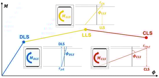
Figure 1.
Moment-curvature relationship of a column section with the corresponding Limit State criteria for Damage limitation Limit State (DLS, tension steel yielding), Life safety Limit State (LLS, concrete cover crushing), and Collapse prevention Limit State (CLS, concrete core crushing).
For rectangular sections with symmetrical reinforcement, these equations are given in Table 1 (further elaborated from [17]), with the notation in Figure 2, where is the section effective depth, is the section width, is the section effective depth after concrete cover spalling, is the tension area of the longitudinal reinforcement, is the area of the transverse reinforcement, and is the transverse reinforcement spacing.

Table 1.
Flexural failure: equations for resisting moment and curvature at three LSs for the case of rectangular sections with symmetric reinforcement.
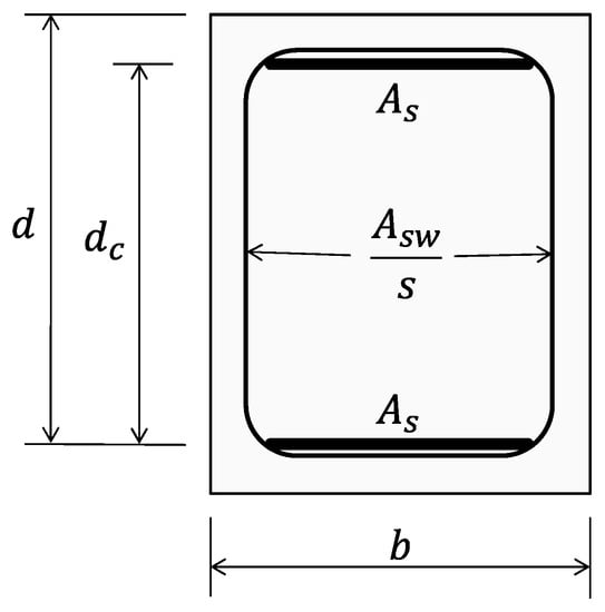
Figure 2.
Cross-section with geometric parameters.
Where is the steel yield strain, is the concrete strain, is the concrete strength, is the longitudinal reinforcement mechanical ratio, and is the normalized axial load, the latter two given as, respectively:
Moreover, is the confining stress normalized with respect to the characteristic concrete strength , and is the concrete strength increase due to confinement, given as:
If needed, the sectional curvature ductility at CLS can be calculated as:
2.3. Column Capacity at
A column is considered as a series system of flexural plastic hinges, column shear, and joints shear.
The flexural force-displacement diagram of a column is obtained by considering, both, the rotations of the two end plastic hinges, which follow the above-described sectional moment-curvature diagram, and the elastic deformation of the column between them. The so-obtained purely flexural response of the column is then compared to its shear capacity and the joints’, to obtain the actual capacity of the column.
The column shear and displacement corresponding to the three Limit States are obtained from equilibrium and compatibility as:
where the elastic stiffness is:
where is the flexural capacity at , is the element height, is the curvature capacity at , is the concrete mean elastic modulus, is the section moment of inertia, and is the plastic hinge length, given, for example, as:
The column shear capacity is computed as:
where is the transverse reinforcement mechanical ratio:
with being the transverse reinforcement area, while is the concrete compressive strength reduction factor, and is a coefficient depending on the normalized axial load , as follows:
The joint shear capacity is computed as:
where is in Figure 2, is the joint effective width, and with in MPa and for internal joints and for external joints.
2.4. Story Capacity at
A story is considered as a parallel system of columns.
The -th interstorey drift capacity and the corresponding resultant force at is determined when the first column attains the corresponding Limit State:
where is the -th column displacement at and is the -th column force at .
The -th interstorey secant stiffness is:
2.5. Frame Capacity at x = D, L, C
The frame can be represented as a series system (a so-called “stick model”) of storeys, where each storey mass is located at height (Figure 3) and where the connecting elements follow the respective trilinear story behavior, obtained from the trilinear columns behaviors, in turn obtained from the trilinear sectional behaviors, as explained in the previous sections.
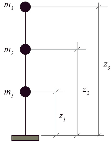
Figure 3.
Frame as a stick-model series system.
In such system, the lateral forces are applied along the frame height according to the shape , which can be taken as either one of the following (height-proportional or mass-proportional):
where it should be noticed that for both.
From the applied force shape , the interstorey shear shape is found as:
The elastic interstorey displacement shape can be found as:
with being the -th story elastic stiffness at .
The frame displacement capacity and resulting base shear at are determined when the first storey attains the corresponding Limit State:
where is the -th interstorey drift in Equation (12) at and is the interstorey shear in Equation (13), taken at the interstorey satisfying Equation (18), denoted with .
3. Determination of Displacement Demand on a 2D Frame
3.1. Simplified Modal Analysis
The first modal shape can be taken equal to the displacement shape. In “stick models” with evenly distributed masses along the height, this is a reasonable approximation that yields negligible errors (lower than 3% for both the eigenvalue ratio and the eigenvector distance norm). Therefore:
where it should be noticed that, by replacing Equation (17), the maximum value at the top () is naturally equal to 1.
The participation factor and the fundamental period are then found as usual as:
It should be noticed that and are diagonal and banded, respectively, as follows (posing for conciseness ):
This allows rewriting Equations (21) and (22) using only summations, thus simplifying their use, for example, in spreadsheets or hand calculations:
where the effective mass and the effective stiffness are:
3.2. Equivalent SDOF System
The “stick model” of the frame is then transformed into an equivalent single degree of freedom (SDOF) system. The top displacement () and the base shear () of the equivalent SDOF system are obtained from Equations (18) and (19), as follows:
Having elastic stiffness:
3.3. Bilinearization
The SDOF system capacity curve, which has a trilinear shape through DLS, LLS, and CLS, is bilinearized to determine its equivalent yield point, which is found as:
The elastic period of such a bilinearized system is:
3.4. Displacement Demands at x = D, L, C
The displacement demands on the frame system pertaining to are obtained from the elastic displacement spectral ordinates computed at on the displacement spectra pertaining to , as:
where is the period at the onset of the descending branch of the acceleration spectrum, and:
where are the elastic spectral ordinates computed at on the acceleration spectra pertaining to . It is important to notice that the spectral shape changes based on the soil class.
4. Development of Fragility Curves for Frame Typologies
4.1. Definition of Fragility Curve
A fragility curve (FC) is defined as the exceedance probability of a threshold that identifies the attainment of a Limit State for a given intensity measure ():
where the demand is obtained from Equation (35) and the capacity pertaining to different Limit States is in Equation (18). This is one of the merits of this study: instead of using a purposely defined metric, such as, for example, a limit interstorey drift, the global displacement capacity is consistently obtained from mechanics-based considerations, as explained in the previous sections, and is therefore related to Limit States. To compare the so-derived fragility curves with those developed in the literature, which are based on qualitative descriptions of damage levels, some correspondence should be found with the Limit States here adopted.
In empirical procedures, descriptive damage scales are preferred in reconnaissance activities to produce post-earthquake damage statistics. Some of the most frequently used damage scales are: HCR [5], HAZUS99 [18], Vision2000 [19], EMS98 [20], and ATC-13 [21]. Table 2, adapted from Ahmad et al. [22], shows a comparison between these damage scales and the Limit States here adopted.
Table 2.
Comparison of various damage scales and the Limit States considered in this study.
Analytical fragility assessment methodologies are commonly based on two main components: (a) the intensity-measure-to-structural-response function, and (b) the structural-response-to-damage-state functions, which result from structural and damage analysis procedures, respectively. Each procedure is affected by uncertainty. When developing FCs from non-linear static analyses, as done in this work, the uncertainty relevant to (b) is explicitly accounted for in all structural parameters: material properties, element sizes, and reinforcement details. The uncertainty related to (a), which is mainly due to record-to-record variability, can be added a posteriori using, for example, the statistically assessed values suggested in FEMA P695 [23]. On the other hand, when developing FCs from non-linear dynamic analyses, the record-to-record uncertainty is explicitly accounted for, whereas including the uncertainty relevant to (b) requires significant computational effort and is usually avoided, under the common assumption that uncertainties of (a) largely exceed uncertainties of (b).
4.2. Selection of Frame Typologies
The frame typologies considered in this study are classified based on the number of storeys, ranging from 1 to 5, and then sub-classified based on the number of bays and bay lengths as given in Table 3 and Figure 4. For each frame typology, two sub-typologies have been considered, representing two different construction periods, 1991–2000 denoted as “new”, and 1961–1970 denoted as “old”. Each sub-typology is characterized by a different range of material properties, concrete strength , steel strength , and of shear reinforcement, stirrup spacing , stirrup diameter and flexural reinforcement (Table 4).
Table 3.
Global geometry parameters of the frame typologies in Figure 4.
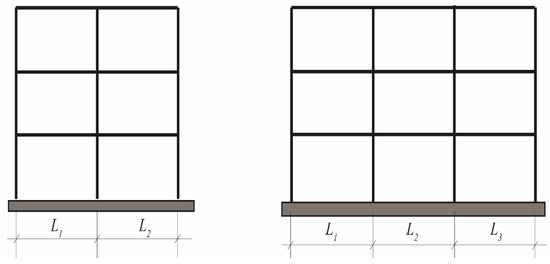
Figure 4.
Geometry of the frame typologies. Number of storeys ranges from 1 to 5, while bay spans are given in Table 3.
Table 4.
Ranges adopted for material properties and reinforcement for the two considered sub-typologies.
4.3. Effects of Soil Class and Location
Fragility Curves (FC) of a given building typology are affected by the soil class. For the purpose of this study, three soil classes have been considered, following the definition in the Italian Building Code (NTC 2018) [24], depending on the equivalent shear wave velocity (in m/s): A (), B (), and C (). To each soil category corresponds a set of coefficients, namely, and , that define the elastic spectral shape. The values of these coefficients are provided in the Italian Building Code (NTC 2018) [24] for nine different return periods, with linear interpolation to obtain and for intermediate periods. This implies that the spectral shape change with the soil class. Therefore, fragility curves developed on a certain soil class need to be adjusted if used in a different one. Such a spectral-shape-changing effect is accounted for in the approach here presented.
As an example, to show such an effect, the FCs pertaining to a given building and location are shown in Figure 5 as obtained on three different soil classes.
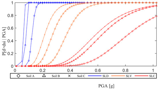
Figure 5.
Soil class influence on FCs for DLS, LLS, and CLS (example shown for Reggio Calabria).
It is worth noticing that the soil class not only affects the median of the FCs, but also the dispersion, so that, for the same value of the PGA, largely different exceedance probabilities are found.
Moreover, it should be noticed that the relationships between and and the return period change from location to location, based on the local hazard. This implies that the spectral shape pertaining to a given soil class for a certain return period varies throughout the territory. Therefore, fragility curves developed at a certain location must be adjusted if used at a different one, even though they refer to the same soil class.
As an example, to show such effect, three different locations in Italy have been chosen: Ferrara, Reggio Calabria, and L’Aquila. For each location, FCs are developed for soil A, B and C. The results in Figure 6 show that, for each soil class considered, the FCs pertaining to a given building change significantly among the three chosen locations.
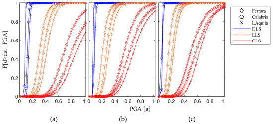
Figure 6.
Location influence on FCs; (a) Soil A; (b) Soil B; and (c) Soil C.
4.4. Monte Carlo Analyses
The fragility curves are built for each selected typology (see Section 4.2) and for each selected soil class (see Section 4.3) through Monte Carlo analysis [25,26]. It is worth mentioning that the location effect has not been accounted for and that a specific location has been selected, i.e., Rome, for the purpose of focusing on the building typologies and the soil effects. The cumulative probability of exceedance of a Limit State (with ) is expressed as function of the horizontal peak ground acceleration, , for reasons of compatibility with the commonly used hazard maps in Italy. For each LS considered, for a given intensity measure , Monte Carlo analyses are performed and a set of displacement-based capacity/demand ratios is obtained and subsequently statistically elaborated as:
where is the exceedance probability of the (with ) for the seismic intensity , with and , corresponding to .
Once the probability for each is obtained, LSE non-linear regression [27,28,29] is carried out to determine the parameters and of the lognormal cumulative distribution function expressed in terms of :
where is the standard normal cumulative distribution function, is the median of the capacity, and is the total coefficient of variation, including both capacity and demand variability.
4.5. Resulting Fragility Curves
The resulting soil-dependent FCs for soil classes A, B and C are shown in Figure 7, Figure 8 and Figure 9, respectively, where it should be noticed that, for each frame typology, a fragility fuse is obtained. The fuse is the result of the variation of the global geometry (Table 3), while the dispersion of each FC is the result of the uncertainties in material properties, beam/column sectional sizes, shear and flexural reinforcement. The effect of the soil class on the FCs at various Limit States (LS) is shown in Figure 10.
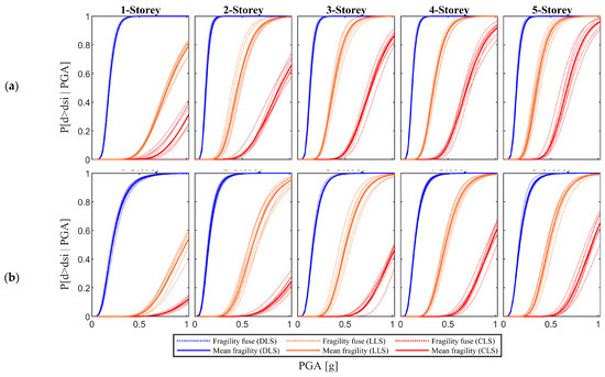
Figure 7.
Resulting fragility curves for soil A; (a) Old; and (b) New.
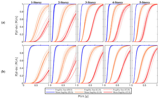
Figure 8.
Resulting fragility curves for soil B; (a) Old; and (b) New.
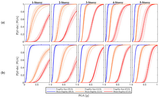
Figure 9.
Resulting fragility curves for soil C; (a) Old; and (b) New.
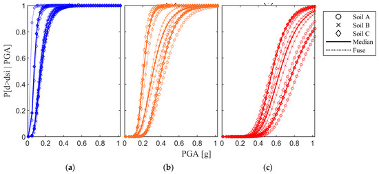
Figure 10.
Soil-aggregated fragility fuses for: (a) DLS (DS1); (b) LLS (DS2); and (c) CLS (DS3).
Building height/number of stories is another parameter that influences the shape of the fragility curves, whereby the fragility of the frames increases with the increasing number of stories. Table 5 reports the FC parameters (mean and coefficient of variation of the PGA-based capacity) for three Limit States, given for different soil classes (A, B, C), different construction types (“Old” and “New”) and with number of storeys ranging from 1 to 5. The mean is given as a range around its mean value ± the distance from the fuse boundaries.
Table 5.
Fragility curve parameters (mean , fuse width around the mean, and coefficient of variation of the PGA-based capacity) for three Damage/Limit States, for three soil types (A, B, C), two construction types (“Old”, Gravity Load Design, and “New”, code-based design) and with number of storeys ranging from 1 to 5.
As a further step, the FCs are aggregated across the soil classes, so as to obtain wider fuses as shown in Figure 10. On passing, these fuses are akin to the observational FCs, which are usually constructed without disaggregating the soil class. Table 6 summarizes these FC parameters (mean and coefficient of variation of the PGA-based capacity) for three Limit States, including soil type variation, for different construction types (“Old” and “New”) and with number of storeys ranging from 1 to 5. The mean is given as a range around its mean value ± the distance from the fuse extremes and is determined as the average of the of soil A, B and C.
Table 6.
Fragility curve parameters including soil type (mean , fuse width around the mean, and coefficient of variation of the PGA-based capacity), for three Damage/Limit States, two construction types (“Old”, Gravity Load Design, and “New”, code-based design) and with number of storeys ranging from 1 to 5.
To this point, the capacity-related variability stems directly from the analysis. As mentioned in Section 4.1, the demand variability should be added as follows:
where is the coefficient of variation due to record-to-record variability, which, according to FEMA P695 [23], can be estimated as 0.2 for DLS and 0.4 for LLS and CLS. Table 7 reports the FC parameters and .
Table 7.
Fragility curve parameters including soil type and demand variability (mean , fuse width around the mean, and total coefficient of variation ), for three Damage/Limit States, two construction types (“Old”, Gravity Load Design, and “New”, code-based design) and with number of storeys ranging from 1 to 5.
4.6. Comparison with Literature Fragility Curves
The validity of the developed analytical FCs is appraised by comparing them with some observational and analytical FCs available in the literature (Figure 11).
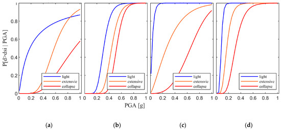
Figure 11.
Fragility curves: observational (a) Del Gaudio et al. [30]; (b) De Luca et al. [31]; (c) Rossetto and Elnashai [5]; and analytical (d) Ahmad et al. [22].
Del Gaudio et al. [30] derived observational-based FCs from the damage distribution data of 7857 buildings in L’Aquila region collected by the Italian Civil Protection Department after the 2009 earthquake. In particular, FCs for low- and medium-rise structures of different types are described. The damage states considered are DS1, DS2, and DS3, which in this work are made to correspond to DLS, LLS and CLS.
De Luca et al. [31] proposed FCs based on the damage data of 131 buildings in the neighborhood of Pettino after L’Aquila earthquake in 2009.
Rossetto and Elnashai [5] developed FCs for European RC structures based on the damage data collected after 19 seismic events, following the HRC damage scale.
Ahmad et al. [22] developed analytical FCs using displacement-based pushover methodology for earthquake loss assessment.
All observational FCs are developed based on statistical analysis of the damage data collected from a set of buildings after seismic events, without distinguishing among different soil classes. This heterogenous collection of data leads to significantly wider dispersions in the fragility fuses than those obtained in this study by disaggregating the soil classes (see Figure 7, Figure 8 and Figure 9). A more consistent comparison is therefore done with respect to the fragility fuses obtained in this study by aggregating the soil classes (see Figure 10).
Such comparison is done in Figure 12, where the blue, orange and red solid lines represent the soil-aggregated fuses for the three LSs. With reference to Figure 10, the lower boundary is determined as the rightmost FC pertaining to soil class A and the upper boundary is determined as the leftmost FC pertaining to soil class C.
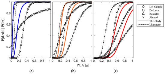
Figure 12.
Comparison between the soil-aggregated FCs and some fragility curves from other authors for: (a) DLS; (b) LLS; and (c) CLS.
In Figure 12, having in mind the correspondence between DS1, DS2 and DS3, to DLS, LLS and CLS, respectively, shown in Table 2, it can be observed that: (a) for DLS, two out of four literature FCs fully fall within the fragility fuse, with the notable exception of that by Del Gaudio et al. [30] which significantly underestimates the DLS-exceedance probability under high PGA values (as a matter of fact, their “light” FC crosses the “extensive” FC, as shown in Figure 11, which is clearly inconsistent), (b) for LLS, basically three out of four literature FCs fall within the fragility fuse, again with the notable exception of that by Del Gaudio et al. [30], which also in this case significantly underestimates the LLS-exceedance probability under high PGA values, (c) for CLS, two out of four literature FCs fall within the fragility fuse, where Ahmad et al. [22] significantly overestimate and Del Gaudio et al. [30] significantly underestimate the CLS-exceedance probability.
5. Conclusions
Fragility Curves are a useful tool for conducting risk analyses at an urban, provincial, or regional scale of territorially diffused building stocks. One of the methods to develop fragility curves relies on statistical processing of the data numerically produced by means of models representing the construction typologies in the region of interest. The so-obtained analytical fragility curves have several advantages over other fragility curves obtained from the statistical treatment of observational damage data, such as, for example: (a) ability to quantitatively define the attainment of certain damage state, as opposed to the qualitative description of observational methods, (b) objectivity of the database, as opposed to the surveyor-dependent observational database, (c) completeness of the database, which is built spanning throughout the range of all basic variables, as opposed to the incomplete database of observational data, (d) flexibility of the database, since analyses can be conducted on any region, even for those where no observational data are available. So far, in the literature, these fragility curves have been obtained: (i) by non-linear dynamic analysis conducted on detailed numerical finite element models, or (ii) with simplified models.
In this study, the second approach was undertaken, by developing a simplified mechanical model that ensures a good compromise between accuracy, representativeness, and computational effort. The simplified model assumes shear-type behavior, which is nonetheless acceptable for most of the existing reinforced concrete buildings. The global displacement-based capacity is analytically derived directly from the local capacity of structural elements and resisting mechanisms, through a simplified closed-form push-over analysis that identifies the attainment of the three global Limit States of interest: Damage, Life Safety, and Collapse. The advantage of the developed method over other simplified pushover analyses in the literature [11,22] is both in its non-iterative approach and in its closed-form nature, which renders the method computationally more efficient, making it suitable for conducting risk studies on a large scale. This allows implementation of the developed assessment methodology, either by hand calculations or in a spreadsheet. The potential of this simplified mechanical model has been shown by applying it on selected typologies of reinforced concrete frames, defined based on number of storeys and construction periods. The latter have been chosen to represent different seismic design compliance levels, from none to full. Within each typology, frames have been randomly generated by varying global and local geometry parameters, reinforcement quantities and material properties, within ranges that are representative of the Italian construction practice in different periods.
Moreover, in this study, a fundamental issue that has been dealt with is the following: fragility curves pertaining to a given typology/building differ depending on the location and the soil class. This is because different locations are characterized by different hazard curves and because different soil classes are characterized by different spectral shapes. These combined effects produce significant changes in the fragility curves, which cannot be accounted for in a simplistic way.
Bearing this in mind, analytical fragility curves for different building typologies have been derived for different soil classes and the parameters of the fitted lognormal curves are summarized in Table 5, where only the within-typology variability is considered, Table 6, where the soil influence is also included, and Table 7, where the demand variability is also included. Such curves have been compared with some observational and analytical curves from the literature, showing acceptable agreement.
The main conclusions drawn from this study can be summarized as follows:
- Location and soil class influence: when developing analytical fragility curves, the influence of the local hazard curve and of the local soil class must be considered. FCs pertaining to the same typology/building change when used at different locations and/or on different soil classes. This induces significant errors on risk and scenario studies at the territorial level. To carry out this study in a more effective manner, a strategy is under development aiming at transforming, through analytical closed-form functions, FCs developed on a certain location and soil class to another one. This is beyond the scope of the present study and will be discussed and presented in a future article.
- Construction age: RC frames fragility is significantly dependent on the construction age when it spans from pre-seismic-code to seismic-code periods. The fragility curves of the two epochs provide insightful information about the vulnerability features of the structures with respect to their construction age.
- Building height: the building height/number of stories is a crucial parameter to the evaluation of the fragility curves, since the LS-exceedance probability increases with the height/number of stories (here, studied only up to five). Thus, it is effectively used as a key parameter to define different building typologies.
Author Contributions
Conceptualization, R.R.R., V.B. and G.M.; methodology, R.R.R., V.B. and G.M.; software, R.R.R.; validation, R.R.R. and G.M.; writing—original draft preparation, R.R.R.; writing—review and editing, G.M.; supervision, G.M. and V.B. All authors have read and agreed to the published version of the manuscript.
Funding
This research was funded within the project DPC-ReLUIS 2019-21.
Institutional Review Board Statement
Not applicable.
Informed Consent Statement
Not applicable.
Data Availability Statement
Data is contained within the article.
Conflicts of Interest
The authors declare no conflict of interest.
References
- Jackson, J. Fatal attraction: Living with earthquakes, the growth of villages into megacities, and earthquake vulnerability in the modern world. Philos. Trans. R. Soc. A Math. Phys. Eng. Sci. 2006, 364, 1911–1925. [Google Scholar] [CrossRef] [PubMed]
- Meroni, F.; Squarcina, T.; Pessina, V.; Locati, M.; Modica, M.; Zoboli, R. A Damage Scenario for the 2012 Northern Italy Earthquakes and Estimation of the Economic Losses to Residential Buildings. Int. J. Disaster Risk Sci. 2017, 8, 326–341. [Google Scholar] [CrossRef] [Green Version]
- Dunand, F.; Gueguen, P. Comparison between seismic and domestic risk in moderate seismic hazard prone region: The Grenoble City (France) test site. Nat. Hazards Earth Syst. Sci. 2012, 12, 511–526. [Google Scholar] [CrossRef] [Green Version]
- Rota, M.; Penna, A.; Strobbia, C.; Magenes, G. Post-Earthquake Survey Data. In Proceedings of the 14th World Conference on Earthaquke Engineering, Beijing, China, 12–17 October 2008. [Google Scholar]
- Rossetto, T.; Elnashai, A. Derivation of vulnerability functions for European-type RC structures based on observational data. Eng. Struct. 2003, 25, 1241–1263. [Google Scholar] [CrossRef]
- Czarnecki, R. Earthquake Damage to Tall Buildings; MIT Department of Civil Engineering: Cambridge, MA, USA, 1973. [Google Scholar]
- Di Trapani, F.; Malavisi, M. Seismic fragility assessment of infilled frames subject to mainshock/aftershock sequences using a double incremental dynamic analysis approach. Bull. Earthq. Eng. 2018, 17, 211–235. [Google Scholar] [CrossRef]
- Basone, F.; Cavaleri, L.; Di Trapani, F.; Muscolino, G. Incremental dynamic based fragility assessment of reinforced concrete structures: Stationary vs. non-stationary artificial ground motions. Soil Dyn. Earthq. Eng. 2017, 103, 105–117. [Google Scholar] [CrossRef]
- Bianco, V.; Granati, S. Expeditious seismic assessment of existing moment resisting frame reinforced concrete buildings: Proposal of a calculation method. Eng. Struct. 2015, 101, 715–732. [Google Scholar] [CrossRef]
- Borzi, B.; Pinho, R.J.S.M.; Crowley, H. Simplified pushover-based vulnerability analysis for large-scale assessment of RC buildings. Eng. Struct. 2008, 30, 804–820. [Google Scholar] [CrossRef]
- Sullivan, T.J.; Saborio-Romano, D.; O’Reilly, G.J.; Welch, D.P.; Landi, L. Simplified Pushover Analysis of Moment Resisting Frame Structures. J. Earthq. Eng. 2021, 25, 621–648. [Google Scholar] [CrossRef]
- Del Gaudio, C.; Ricci, P.; Verderame, G.M.; Manfredi, G. Observed and predicted earthquake damage scenarios: The case study of Pettino (L’Aquila) after the 6th April 2009 event. Bull. Earthq. Eng. 2016, 14, 2643–2678. [Google Scholar] [CrossRef]
- Del Gaudio, C.; Ricci, P.; Verderame, G.M. A class-oriented large scale comparison with postearthquake damage for Abruzzi Region. In Proceedings of the 6th International Conference on Computational Methods in Structural Dynamics and Earthquake Engineering Methods in Structural Dynamics and Earthquake Engineering, Rhodes Island, Greece, 15–17 June 2017. [Google Scholar] [CrossRef] [Green Version]
- Buratti, N.; Minghini, F.; Ongaretto, E.; Savoia, M.; Tullini, N. Empirical seismic fragility for the precast RC industrial buildings damaged by the 2012 Emilia (Italy) earthquakes. Earthq. Eng. Struct. Dyn. 2017, 46, 2317–2335. [Google Scholar] [CrossRef]
- Rota, M.; Penna, A.; Strobbia, C. Processing Italian damage data to derive typological fragility curves. Soil Dyn. Earthq. Eng. 2008, 28, 933–947. [Google Scholar] [CrossRef]
- Kappos, A.J.; Panagopoulos, G.; Panagiotopoulos, C.; Penelis, G. A hybrid method for the vulnerability assessment of R/C and URM buildings. Bull. Earthq. Eng. 2006, 4, 391–413. [Google Scholar] [CrossRef]
- Petrone, F.; Monti, G. Unified code-compliant equations for bending and ductility capacity of full and hollow rectangular RC sections. Eng. Struct. 2019, 183, 805–815. [Google Scholar] [CrossRef]
- Hazus. Hazus–MH 2.1: Technical Manual. Fed. Emerg. Manag. Agency 2012, 718. Available online: www.fema.gov/plan/prevent/hazus (accessed on 29 June 2021).
- Structural Engineers Association of California. SEAOC-Vision 2000—A Framework for Performance-Based Design Vol I–III; Structural Engineers Association of California: Sacramento, CA, USA, 1995. [Google Scholar]
- Grünthal, G.; Schwarz, J. European Macroseismic Scale 1998 EMS-98; European Seismological Commission: Luxembourg, 1998. [Google Scholar]
- Rojahn, C.; Abel, M.A.; Ayres, J.M.; Blume, J.A.; Sharpe, R.L.; Brogan, G.E.; Cassano, R.; Christensen, T.M.; Degenkoib, H.J.; Scholl, R.E.; et al. ATC-13 Earthquake Damage Evaluation Data for California; Applied Technology Council: Redwood, CA, USA, 1985. [Google Scholar]
- Ahmad, N.; Crowley, H.; Pinho, R. Analytical Fragility Functions for Reinforced Concrete and Masonry Buildings and Building Aggregates of Euro-Mediterranean Regions; Department of Civil Engineering University of California: Berkeley, CA, USA, 2011. [Google Scholar]
- FEMA. P.695-Quantification of Building Seismic Performance Factors; Federal Emergency Management Agency: Washington, DC, USA, 2009.
- NTC. Aggiornamento Delle «Norme Tecniche per le Costruzioni»; Ministry of Transport and Infrastructure: Rome, Italy, 2018.
- Ang, A.H.S.; Tang, W.H. Probability Concepts in Engineering Planning and Design; John Wiley & Sons: New York, NY, USA, 1975; Volume 1. [Google Scholar]
- Ang, A.H.S.; Tang, W.H. Probability Concepts in Engineering Planning and Design, Volume 2: Decision, Risk, and Reliability; John Wiley & Sons, Inc., 605 Third Ave.: New York, NY, USA, 1984. [Google Scholar]
- Rossetto, T.; Ioannou, I.; Grant, D. Existing Empirical Fragility and Vulnerability Functions: Compendium and Guide for Selection; GEM Foundation: Pavia, Italy, 2013. [Google Scholar]
- Rossetto, T.; Ioannou, I.; Grant, D.; Maqsood, T. Guidelines for Empirical Vulnerability Assessment; GEM Foundations: Pavia, Italy, 2014. [Google Scholar]
- Ioannou, I.; Rossetto, T.; Grant, D. Use of regression analysis for the construction of empirical fragility curves. In Proceedings of the 15th World Conference on Earthquake Engineering, Lisbon, Portugal, 24–28 September 2012. [Google Scholar]
- Del Gaudio, C.; De Martino, G.; Di Ludovico, M.; Manfredi, G.; Prota, A.; Ricci, P.; Verderame, G.M. Empirical fragility curves from damage data on RC buildings after the 2009 L’Aquila earthquake. Bull. Earthq. Eng. 2016, 15, 1425–1450. [Google Scholar] [CrossRef]
- De Luca, F.; Verderame, G.M.; Manfredi, G. Analytical versus observational fragilities: The case of Pettino (L’Aquila) damage data database. Bull. Earthq. Eng. 2014, 13, 1161–1181. [Google Scholar] [CrossRef] [Green Version]
Publisher’s Note: MDPI stays neutral with regard to jurisdictional claims in published maps and institutional affiliations. |
© 2021 by the authors. Licensee MDPI, Basel, Switzerland. This article is an open access article distributed under the terms and conditions of the Creative Commons Attribution (CC BY) license (https://creativecommons.org/licenses/by/4.0/).