
Assessment of the Density Loss in Anobiid Infested Pine Using X-ray Micro-Computed Tomography

 ,
,  ,
,  ,
,  ,
,  and
and
Abstract
1. Introduction
2. Materials and Methods
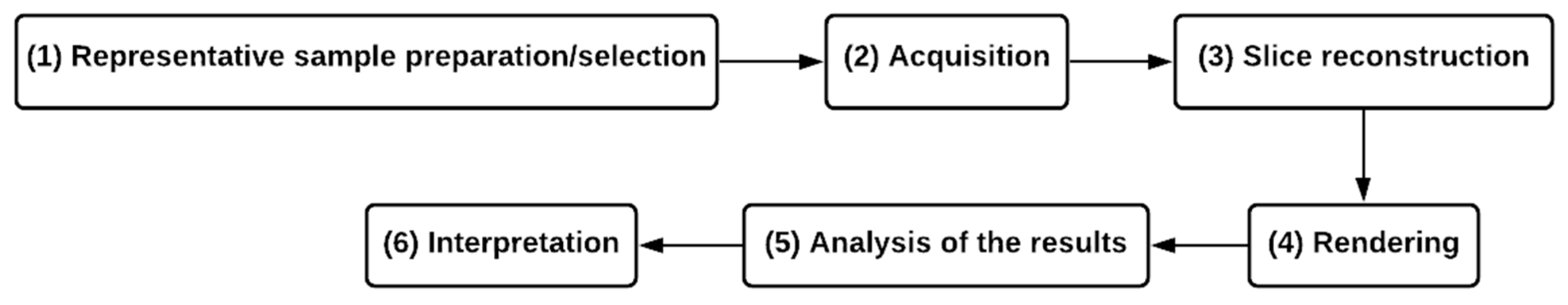
2.1. X-Ray Micro-Computed Tomography Study
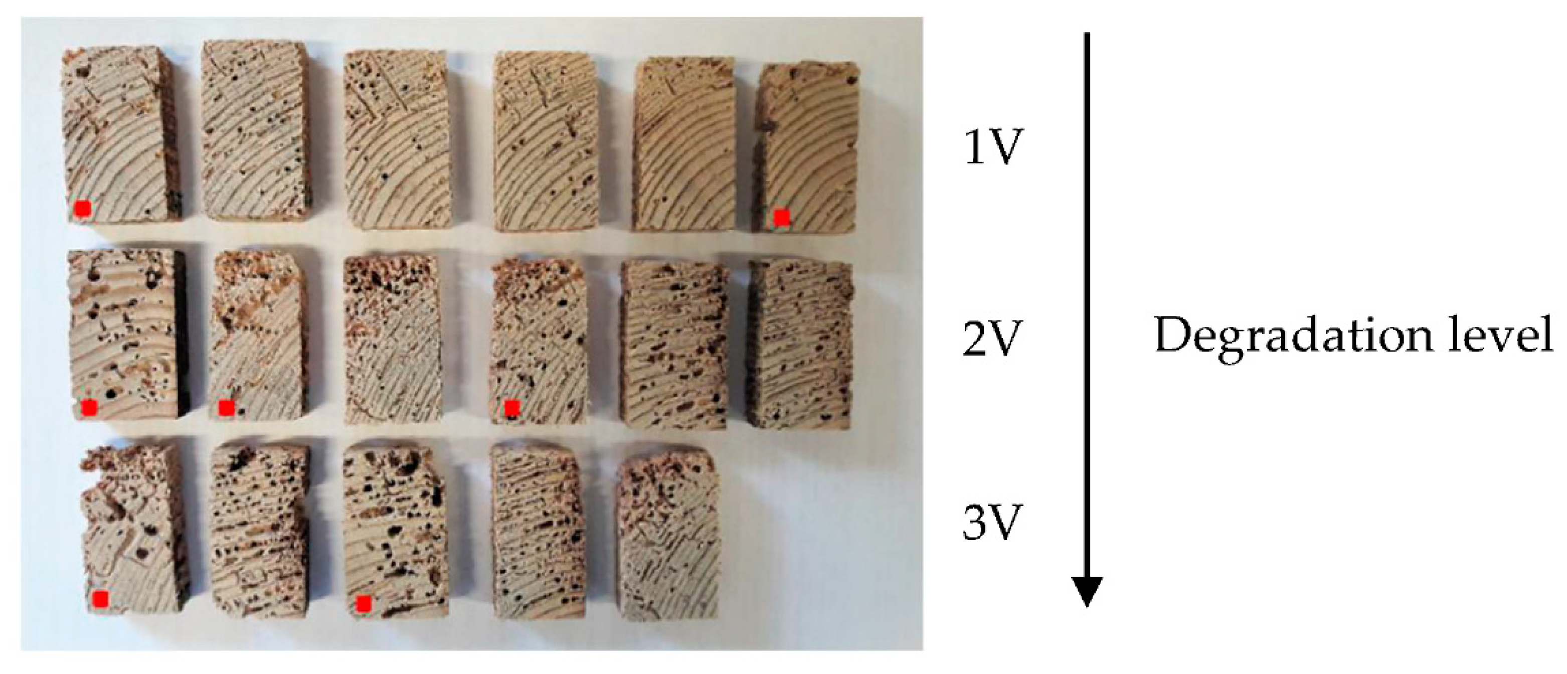
2.2. Representative Sample Preparation/Selection
2.3. Scanning Procedure (Acquisition)
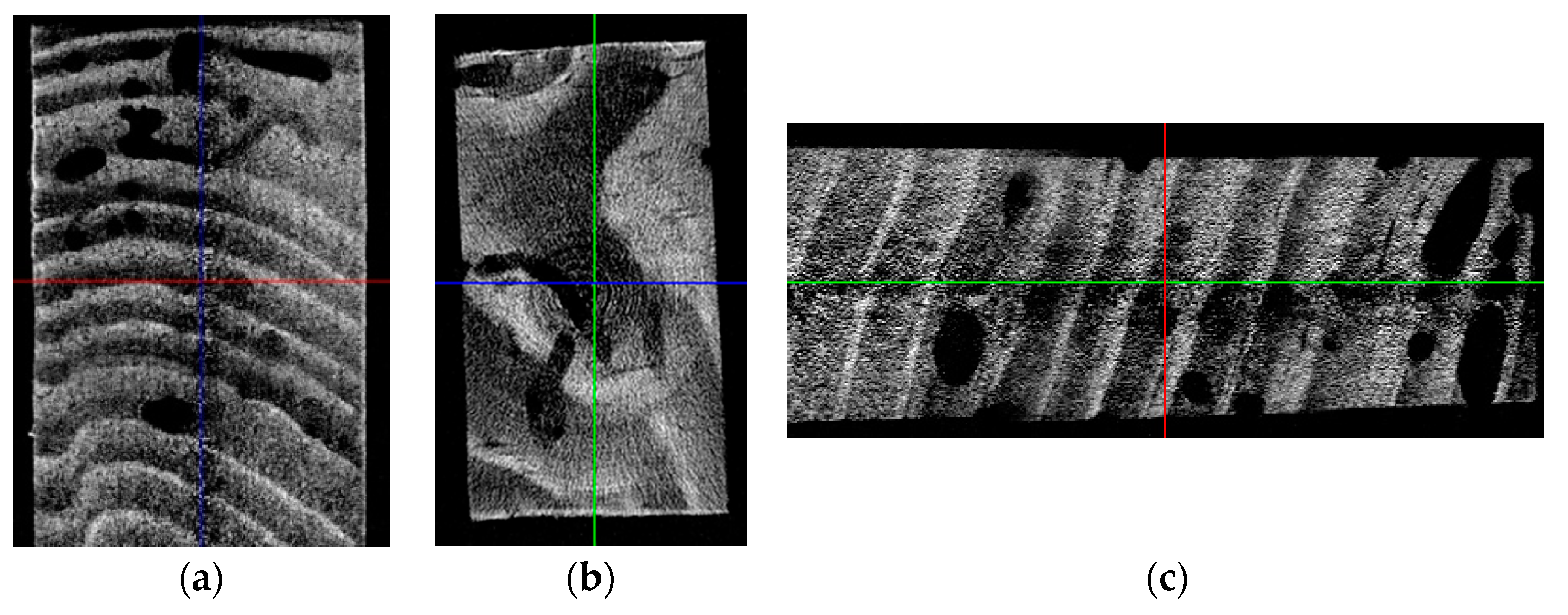
2.4. Reconstruction
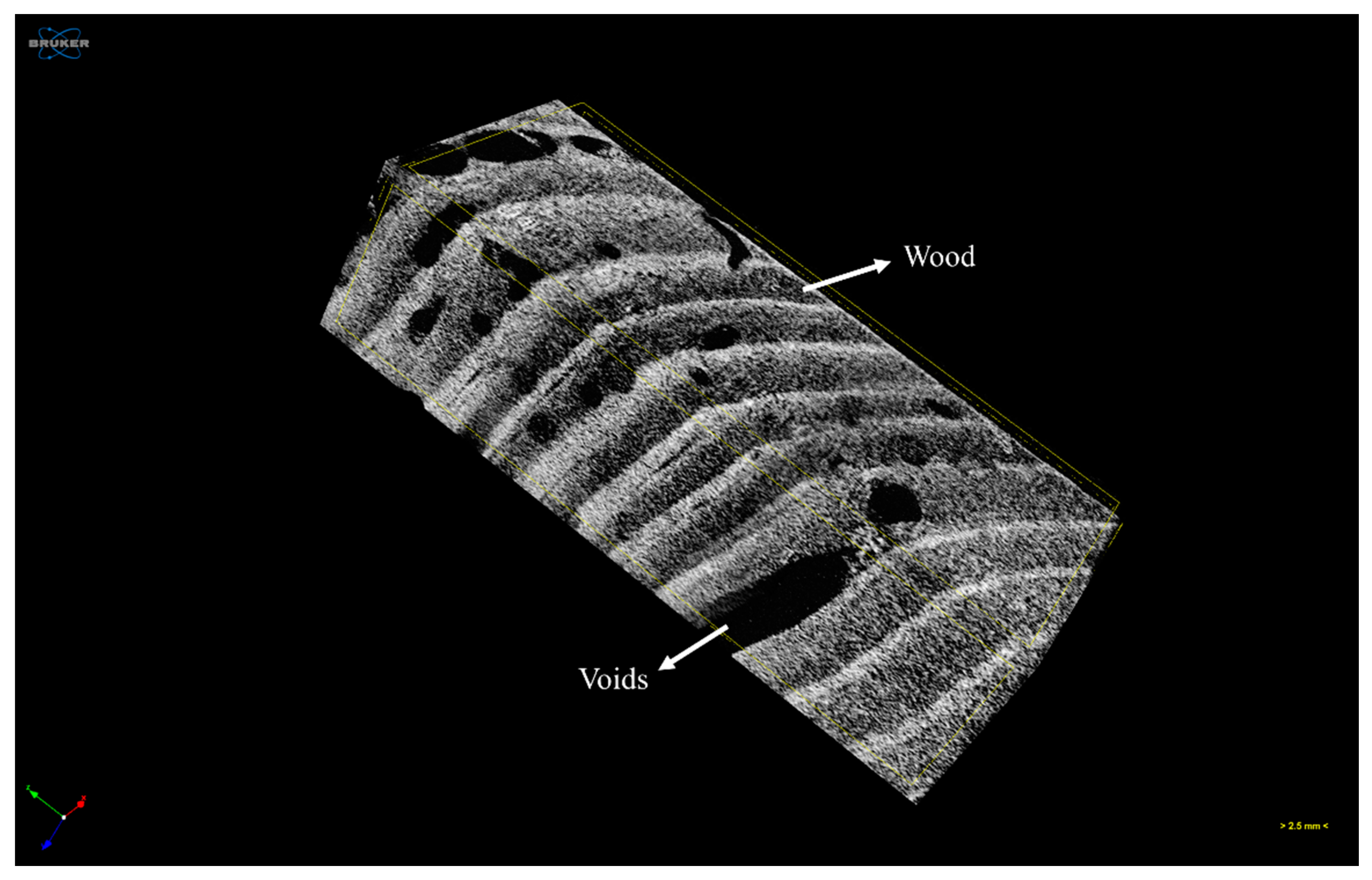
2.5. Analysis
3. Results and Discussion
4. Conclusions
Author Contributions
Funding
Institutional Review Board Statement
Informed Consent Statement
Data Availability Statement
Conflicts of Interest
References
- Parracha, J.L.; Pereira, M.F.C.; Maurício, A.; Machado, J.S.; Faria, P.; Nunes, L. It’s what’s inside that counts: An assessment method to measure the residual strength of anobiids infested timber using micro-computed tomography. In Proceedings of the SHATIS’2019–5th International Conference on Structural Health Assessment of Timber Structures, Guimarães, Portugal, 25–27 September 2019; p. 10. [Google Scholar]
- Eaton, R.A.; Hale, M.D.C. Wood: Decay, Pests and Protection; Chapmman & Hall Ltd.: London, UK, 1993. [Google Scholar]
- EN 350:2016. Durability of Wood and Wood-Based Products–Testing and Classification of the Durability to Biological Agents of Wood and Wood-Based Materials; European Committee for Standardization: Brussels, Belgium, 2016. [Google Scholar]
- Bravery, A.F.; Berry, R.W.; Carey, J.K.; Cooper, D.E. Recognising Wood Rot and Insects Damage in Buildings; Building Research Establishment: Garston, UK, 1992. [Google Scholar]
- Parracha, J.; Pereira, M.F.C.; Maurício, A.; Machado, J.S.; Faria, P.; Nunes, L. A semi-destructive assessment method to estimate the residual strength of maritime pine structural elements degraded by anobiids. Mater. Struct. 2019, 52, 1–11. [Google Scholar] [CrossRef]
- Nunes, L.; Parracha, J.; Faria, P.; Palma, P.; Pereira, M.F.C.; Maurício, A. Towards an assessment tool of anobiid damage of pine timber structures. In Proceedings of the IABSE Symposium 2019 Guimarães “Towards a Resilient Built Environment-Risk and Asset Management”, Guimarães, Portugal, 27–29 March 2019; p. 8. [Google Scholar]
- Cruz, H.; Machado, J.S. Effects of beetle attack on the bending and compression strength properties of pine wood. Adv. Mater. Res. 2013, 778, 145–151. [Google Scholar] [CrossRef]
- Gilfillan, J.R.; Gilbert, S.G. Development of a technique to measure the residual strength of woodworm infested timber. Constr. Build. Mater. 2001, 15, 381–388. [Google Scholar] [CrossRef]
- Cruz, H.; Yeomans, D.; Tsakanika, E.; Macchioni, N.; Jorissen, A.; Touza, M.; Mannucci, M.; Lourenço, P.B. Guidelines for on-site assessment of historic timber structures. Int. J. Archit. Herit. 2015, 9, 277–289. [Google Scholar] [CrossRef]
- Cuartero, J.; Cabaleiro, M.; Sousa, H.S.; Branco, J.M. Tridimensional parametric model for prediction of structural safety of existing timber roofs using laser scanner and drilling resistance tests. Eng. Struct. 2019, 185, 58–67. [Google Scholar] [CrossRef]
- Piazza, M.; Riggio, M. Visual strength-grading and NDT of timber in traditional structures. J. Build. Apprais. 2008, 3, 267–296. [Google Scholar] [CrossRef]
- Lechner, T.; Sandin, Y.; Kliger, R. Assessment of density in timber using X-ray equipment. Int. J. Archit. Herit. 2013, 7, 416–433. [Google Scholar] [CrossRef]
- Kandemir-Yucel, A.; Tavukcuoglu, A.; Caner-Saltik, E.N. In situ assessment of structural timber elements of a historic building by infrared thermography and ultrasonic velocity. Infrared Phys. Technol. 2007, 49, 243–248. [Google Scholar] [CrossRef]
- Rivera-Gómez, C.; Galán-Marín, C. In situ assessment of structural timber elements of a historic building by moisture content analyses and ultrasonic velocity tests. Int. J. Hous. Sci. 2013, 37, 33–42. [Google Scholar]
- Kordatos, E.Z.; Exarchos, D.A.; Stavrakos, C.; Moropoulou, A.; Matikas, T.E. Infrared thermographic inspection of murals and characterization of degradation in historic monuments. Constr. Build. Mater. 2013, 48, 1261–1265. [Google Scholar] [CrossRef]
- Feio, A.; Machado, J.S. In-situ assessment of timber structural members: Combining information from visual strength grading and NDT/SDT methods–A review. Constr. Build. Mater. 2015, 101, 1157–1165. [Google Scholar] [CrossRef]
- Baird, E.; Taylor, G. X-ray micro-computed tomography. Curr. Biol. Mag. 2017, 27, 283–293. [Google Scholar] [CrossRef] [PubMed]
- Wei, Q.; Leblon, B.; La Rocque, A. On the use of X-ray computed tomography for determining wood properties: A review. Can. J. For. Res. 2011, 41, 11. [Google Scholar] [CrossRef]
- Farinha, A.O.; Branco, M.; Pereira, M.F.C.; Auger-Rozenberg, M.; Maurício, A.; Yart, A.; Guerreiro, V.; Sousa, E.M.R.; Roques, A. Micro X-ray computed tomography suggests cooperative feeding among adult invasive bugs Leptoglosus occidentalis on mature seeds of stone pine Pinus pinea. Agric. For. Entomol. 2018, 20, 18–27. [Google Scholar] [CrossRef]
- Fuchs, A.; Schreyer, A.; Feuerbach, S.; Korb, J. A new technique for termite monitoring using computer tomography and endoscopy. Int. J. Pest Manag. 2004, 50, 63–66. [Google Scholar] [CrossRef]
- Himmi, S.K.; Yoshimura, T.; Yanase, Y.; Oya, M.; Torigoe, T.; Imazu, S. X-ray tomography analysis of the initial structure of the royal chamber and the nest-founding behaviour of the drywood termite Incisitermes minor. J. Wood Sci. 2014, 60, 453–460. [Google Scholar] [CrossRef]
- Kigawa, R.; Torigoe, T.; Imazu, S.; Honda, M.; Harada, M.; Komine, Y.; Kawanobe, W. Detection of insects in wooden objects by X-ray CT scanner. Sci. Conserv. 2009, 48, 223–231. [Google Scholar] [CrossRef]
- Watanabe, H.; Yanase, Y.; Fujii, Y. Evaluation of larval growth process and bamboo consumption of the bamboo powder-post beetle Dinoderus minutus using X-ray computed tomography. J. Wood Sci. 2015, 61, 171–177. [Google Scholar] [CrossRef]
- Charles, F.; Coston-Guarini, J.; Guarini, J.; Lantoine, F. It’s what’s inside that counts: Computer-aided tomography for evaluating the rate and extent of wood consumption by shipworms. J. Wood Sci. 2018, 64, 427–435. [Google Scholar] [CrossRef]
- ISO 13061-1:2014. Physical and Mechanical Properties of Wood–Test Methods for Small Clear Wood Specimens–Part 1. Determination of Moisture Content for Physical and Mechanical Tests; International Organization for Standardization: Geneva, Switzerland, 2014. [Google Scholar]
- du Plessis, A.; Broeckhoven, C.; Guelpa, A.; Gerard le Roux, S. Laboratory x-ray micro-computed tomography: A user guideline for biological samples. Gigascience 2017, 6, 1–11. [Google Scholar] [CrossRef]
- du Plessis, A.; Boshoff, W.P. A review of X-ray computed tomography of concrete and asphalt construction materials. Constr. Build. Mater. 2019, 199, 637–651. [Google Scholar] [CrossRef]
- Singhal, A.; Grande, J.C.; Zhou, Z. Micro/nano CT for visualization of internal structures. Microsc. Today 2013, 21, 16–22. [Google Scholar] [CrossRef]
- Campbell, G.M.; Sophocleous, A. Quantitative analysis of bone and soft issue by micro-computed tomography: Applications to ex vivo and in vivo studies. BoneKEY Rep. 2014, 3, 564. [Google Scholar] [CrossRef]
- Maurício, A.; Figueiredo, C.; Alves, C.; Pereira, M.F.C.; Aires-Barros, L.; Neto, J.A.N. Non-destructive microtomography-based imaging and measuring laboratory-induced degradation of travertine, a random heterogeneous geomaterial used in urban heritage. Environ. Earth Sci. 2013, 69, 1471–1480. [Google Scholar] [CrossRef]
- Ketcham, R.A.; Carlson, W.D. Acquisition, optimization and interpretation of X-ray computed tomography imagery: Applications to the geosciences. Comput. Geosci. 2001, 27, 381–400. [Google Scholar] [CrossRef]
- Cnudde, V.; Cnudde, J.P.; Dupuis, C.; Jacobs, P.J.S. X-ray micro tomography used for the localisation of water repellents and consolidants inside natural building stones. Mater. Charact. 2004, 53, 259–271. [Google Scholar] [CrossRef]
- Ketcham, R.A.; Iturrino, G.J. Nondestructive high-resolution visualization and measurement of anisotropic effective porosity in complex lithologies using high-resolution X-ray computed tomography. J. Hydrol. 2005, 302, 92–106. [Google Scholar] [CrossRef]
- Rozenbaum, O.; Bergounioux, M.; Maurício, A.; Figueiredo, C.; Alves, C.; Barbanson, L. Versatile Three-Dimensional Denoising and Segmentation Method of X-ray Tomographic Images: Applications to Geomaterials Characterizations. Preprint 2016. Available online: https://hal.archives-ouvertes.fr/hal-01255507 (accessed on 13 April 2021).
- Maurício, A.; Figueiredo, C.; Pereira, M.F.C.; Bergounioux, M.; Rozenbaum, O. Assessment of stone heritage decay by X-ray computed microtomography: II–a case of study of Portuguese limestones. Microsc. Microanal. 2015, 21, 162–163. [Google Scholar] [CrossRef]
- Parkinson, I.H.; Badiei, A.; Fazzalari, N.L. Variation in segmentation of bone from micro-CT imaging: Implications for quantitative morphometric analysis. Australas. Phys. Eng. Sci. Med. 2008, 31, 160–164. [Google Scholar] [CrossRef]
- Brozovsky, J.; Brozovsky, J.J.; Zach, J. An assessment of the condition of timber structures. In Proceedings of the 9th International Conference on NDT of Art, Jerusalem, Israel, 25–30 May 2008. [Google Scholar]


| Parameters | |||
|---|---|---|---|
| Maximum resolution | 2 μm | Voltage | 60 kV |
| Filament current | 165 μA | Number of images | 288 |
| Angle of rotation | 0.7° | Filters | Al 0.5 mm |
| Voxel Size | 18.09 μm | File type | 16-bit |
| Parameter | Description | Suggested Setting |
|---|---|---|
| Smoothing | Smooth images and removes noise | Width; 3 pixels |
| Beam-hardening factor correction | Correct for the absorption of lower-energy X-ray on the outside of the specimen | 30–55% |
| Ring artefact reduction | Correct for the nonlinear behavior of pixels causing ring artefacts | ≈20 |
| Parameter | Description | Suggested Setting |
|---|---|---|
| Thresholding | Segments the foreground from background to binary images | Global; low level 17, high level 255 |
| Despeckle | Removes speckles from binary images | Remove white speckles <500 voxels; remove black speckles <150 voxels |
| Morphological operations | Fills the holes and closes the pores | 2D space: Closing; Kernel round, radius 5 |
| Degradation Level | Sample | Total Volume | Wood Volume | Lost Material | Weight |
|---|---|---|---|---|---|
| cm3 | cm3 | % | g | ||
| Level 1 | 1.1 | 8.798 | 7.868 | 10.57 | 4.541 |
| 1.2 | 9.250 | 8.339 | 9.85 | 4.776 | |
| 1.3 | 8.913 | 8.074 | 9.41 | 4.520 | |
| 1.4 | 9.168 | 8.299 | 9.48 | 4.308 | |
| 1.5 | 7.352 | 6.731 | 8.45 | 4.360 | |
| 1.6 | 7.576 | 6.293 | 16.94 | 3.455 | |
| Level 2 | 2.1 | 8.529 | 7.811 | 8.42 | 4.763 |
| 2.2 | 7.020 | 5.413 | 22.89 | 2.912 | |
| 2.3 | 7.291 | 5.865 | 19.56 | 2.807 | |
| 2.4 | 6.319 | 4.854 | 23.18 | 2.152 | |
| 2.5 | 8.179 | 7.158 | 12.48 | 3.862 | |
| 2.6 | 7.021 | 6.022 | 14.23 | 2.988 | |
| Level 3 | 3.1 | 8.774 | 7.071 | 19.41 | 3.412 |
| 3.2 | 8.631 | 6.309 | 26.90 | 2.544 | |
| 3.3 | 7.216 | 6.260 | 13.25 | 3.084 | |
| 3.4 | 8.011 | 6.224 | 22.31 | 3.212 | |
| 3.5 | 7.154 | 5.595 | 21.79 | 2.782 |
| Degradation Level | 1V | 2V | 3V | |
|---|---|---|---|---|
| Number of samples | 6 | 6 | 5 | |
| Volume (cm3) | Total | 8.452 | 7.393 | 7.957 |
| Wood | 7.601 | 6.187 | 6.292 | |
| Lost material (%) | 10.78 ± 3.52 | 16.79 ± 5.49 | 20.73 ± 4.87 | |
| Weight (g) | 4.327 | 3.247 | 3.007 | |
| Densities (kg/m3) | Original | 571 ± 65 | 518 ± 83 | 481 ± 44 |
| Residual | 510 ± 45 | 433 ± 64 | 380 ± 36 | |
| Loss | 10.7 ± 2.89 | 16.4 ± 4.68 | 20.9 ± 5.65 | |
| Degradation Level | 1 | 2 | 3 | |
|---|---|---|---|---|
| Number of samples | 5 | 7 | 5 | |
| Volume (cm3) | Total | 8.642 | 7.836 | 7.427 |
| Wood | 7.850 | 6.648 | 5.679 | |
| Lost material (%) | 9.12 ± 1.05 | 15.16 ± 2.45 | 23.54 ± 1.84 | |
| Weight (g) | 4.545 | 3.449 | 2.720 | |
| Densities (kg/m3) | Original | 582 ± 74 | 517 ± 62 | 495 ± 45 |
| Residual | 529 ± 53 | 439 ± 70 | 386 ± 28 | |
| Loss | 9.2 ± 0.64 | 15.3 ± 3.5 | 21.9 ± 1.4 | |
Publisher’s Note: MDPI stays neutral with regard to jurisdictional claims in published maps and institutional affiliations. |
© 2021 by the authors. Licensee MDPI, Basel, Switzerland. This article is an open access article distributed under the terms and conditions of the Creative Commons Attribution (CC BY) license (https://creativecommons.org/licenses/by/4.0/).
Share and Cite
Parracha, J.; Pereira, M.; Maurício, A.; Faria, P.; Lima, D.F.; Tenório, M.; Nunes, L. Assessment of the Density Loss in Anobiid Infested Pine Using X-ray Micro-Computed Tomography. Buildings 2021, 11, 173. https://doi.org/10.3390/buildings11040173
Parracha J, Pereira M, Maurício A, Faria P, Lima DF, Tenório M, Nunes L. Assessment of the Density Loss in Anobiid Infested Pine Using X-ray Micro-Computed Tomography. Buildings. 2021; 11(4):173. https://doi.org/10.3390/buildings11040173
Chicago/Turabian StyleParracha, João, Manuel Pereira, António Maurício, Paulina Faria, Daniel F. Lima, Marina Tenório, and Lina Nunes. 2021. "Assessment of the Density Loss in Anobiid Infested Pine Using X-ray Micro-Computed Tomography" Buildings 11, no. 4: 173. https://doi.org/10.3390/buildings11040173
APA StyleParracha, J., Pereira, M., Maurício, A., Faria, P., Lima, D. F., Tenório, M., & Nunes, L. (2021). Assessment of the Density Loss in Anobiid Infested Pine Using X-ray Micro-Computed Tomography. Buildings, 11(4), 173. https://doi.org/10.3390/buildings11040173