
Seismic and Coastal Vulnerability Assessment Model for Buildings in Chile


Abstract
1. Introduction
2. Materials and Methods
2.1. Seismic Vulnerability Assessment
2.1.1. Calculating the New Building Standard Capacity (%NBS)
- Factor A
- Factor B
- Structural Performance Indicator (SPI) Factors
2.1.2. Building Rating
2.2. Coastal Vulnerability Assessment
- Physical variables
- Average wave height (PV2): The waves’ energy increases as wave height increases, which leads to loss of land area caused by erosion and flooding along the coast. Because of this, coastal areas with high wave heights are considered to be more vulnerable. Therefore, the study of vulnerability based on wave height is an important step in the creation of a tsunami alert and risk management system [41]. Average wave height can be easily obtained from the tide charts generated by the maritime authority [42].
- Tidal range (PV3): Tidal range is the vertical difference between the highest and lowest tides and is related to permanent and intermittent flooding risk. Tidal range can easily be obtained from the tide charts generated by the maritime authority [42].
- Beach width (PV4): Beach width is measured from the backshore’s coordinates to the mean low water mark. Because of variations in tidal range, this parameter was approximately measured using the Google Earth Pro v7.3 [43] application. To obtain a more precise calculation of the width of the beach, maritime authority recommends carrying out a topographic survey of the sector [44].
- Coastal slope (PV5): This variable considers the average slope of each sector, over the line of the shortest distance to the coastline. The lower the slope, the greater the risk for possible flooding caused by a tsunami. Slope is calculated by dividing the difference in elevation by the horizontal difference that exists between the coast and the location under study.
- Distance to water body (PV6): This physical variable corresponds to the shortest existing distance between the closest water body (coastline, river or estuary) and the location under study (in the case of a large area, the centroid of that area is used). The closer the sector is to the coast, the more susceptible it is to damage.
- Coastal protection (PV7): This variable refers to whether the structure is or is not covered by some type of natural (hill, trees or other) or artificial protection. The absence of protection makes the structure more vulnerable.
- Structural variables
- Number of stories (SV1): In the case of tsunami and fluvial floods, this parameter is important for determining a building’s vulnerability, as a higher number of stories allows for the vertical evacuation of people and possessions.
- Structure’s state of conservation (SV2): This variable indicates the state of conservation of buildings within the study area, quantifying its vulnerability. A visual assessment was carried out, considering three categories (good, regular and bad). Good means that all the structural elements (columns, beams and walls) are in perfect condition. Regular indicates that the structural elements have surface cracks or slight deformations. Finally, bad means that the structural elements are cracked, the reinforcement’s covering is detached or there are considerable deformations.
- Structure’s material (SV3): This variable indicates how vulnerable a building is to tsunami and floods based on the materials used for its construction. Three main building typologies were identified in the area of study: reinforced concrete (RC), masonry (M) and timber (T) buildings, in addition to combinations of them (RC + T and M + T). There were also precarious buildings (PB), made of deficient construction materials, typical of impoverished areas in South America. Each one of these typologies was assigned a level of vulnerability, depending on the building material.
- Sociodemographic variables
- Socioeconomic level (SDV1): Although we are evaluating buildings, it is relevant to also examine their inhabitants’ socioeconomic level. While the buildings may be in good condition, the occupants’ capacity for recovering the structures will also be associated with their economic capacity to rehabilitate the structures in case of damage. There are many economic activities that could be negatively affected by coastal flooding, among them sailing, industry, tourism, agriculture, fishing, availability of potable water, private companies located in affected areas, etc. According to McLaughlin and Cooper [45], the selection of socioeconomic variables adds an inherent cultural bias to an index, as it should incorporate factors associated to economic prosperity from the determined productive sector. According to this statement, a coastal vulnerability assessment will be affected by the socioeconomic environment that is directly related to residents’ income. Buildings owned by those with a high socioeconomic status are less vulnerable, as their rehabilitation is easier if the economic resources are available to do so. This is independent of the building’s material or state of conservation. In this study, El-Hattab’s [8] proposal was used, in which socioeconomic level depends on inhabitants’ highest level of education, and subsequently, their occupation.
- Population density (SDV2): It is uncommon to use population as a variable in coastal vulnerability assessment. While authors like Hughes and Brundrit [46] do not include it, they do recognize that a more populated area has greater economic value, reaching the conclusion that other studies should concentrate on the population dynamic and the effects of an increase in urbanization. Gornitz [19,20] also omitted population but indicated that further studies should take the coastal populations into consideration in order to help assess vulnerable areas. Thus, the greater the population density the more susceptible the area of study will be. Information available by block from the 2017 Census [47] was used to obtain the number of inhabitants.
- Weighting factors calculation
2.3. Combined Vulnerability Assessment Model
3. Results
3.1. Case Study 1: Building Assessment
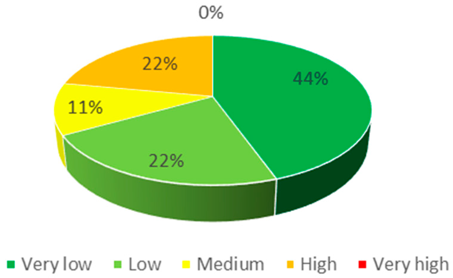
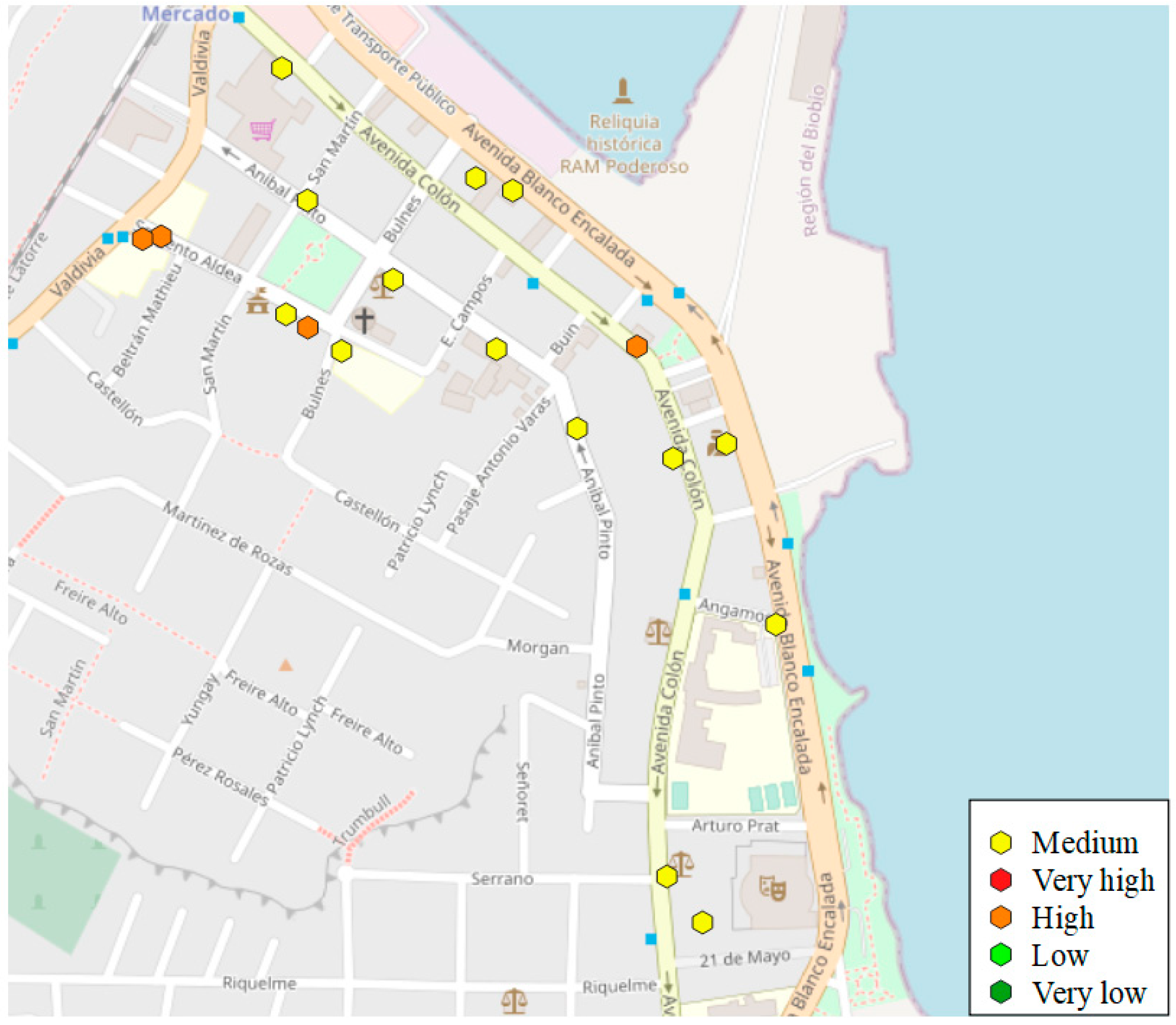
3.2. Case Study 2: Territorial Assessment
4. Discussion
- Basic information (building’s year of construction and soil class) needed to perform SVA was not readily available for the general public and had to be requested through official procedures; it takes 20 business days for an answer to be provided. The SVA could be quickly and easily applied if the municipalities made this information available as a policy.
- Originally, this study considered extensive field work for performing visual inspections of the buildings and collecting sociodemographic data. However, the 2020 world health crisis forced us to redesign these kinds of surveys. Consequently, the visual inspection was done using Google Street View [43] and the sociodemographic parameters were obtained by telephone surveys and census information. Hence, the COVID-19 crisis helped to demonstrate that the proposed methodology does not require extensive field work and most (if not all) the procedures can be performed remotely.
5. Conclusions
Author Contributions
Funding
Institutional Review Board Statement
Informed Consent Statement
Data Availability Statement
Acknowledgments
Conflicts of Interest
References
- Scholz, C.H. The Mechanics of Earthquakes and Faulting; Cambridge University Press: Cambridge, UK, 2002; pp. 300–329. [Google Scholar]
- Atwater, B.F.; Musumi-Rokkaku, S.; Satake, K.; Tsuji, Y.; Ueda, K.; Yamaguchi, D.K. The orphan tsunami of 1700—Japanese clues to a parent earthquake in North America. In Professional Paper; US Geological Survey: Botetourt, VA, USA, 2005. [Google Scholar]
- Cowan, H.; Beattie, G.; Hill, K.; Evans, N.; McGhie, C.; Gibson, G.; Lawrance, G.; Hamilton, J.; Allan, P.; Bryant, M.; et al. The M8.8 Chile earthquake, 27 February 2010. Bull. New Zealand Soc. Earthq. Eng. 2011, 44, 123–166. [Google Scholar] [CrossRef]
- Organización Panamericana de la Salud (OPS). Fundamentos Para la Mitigación de Desastres en Establecimientos de Salud; Serie Miti-gación de Desastres: Washington, DC, USA, 2000. [Google Scholar]
- Astroza, M.; Moroni, M.; Muñoz, M.; Pérez, F. Estudio de la vulnerabilidad sísmica de edificios de vivienda social. In Proceedings of the IX Congreso Chileno de Sismología e Ingeniería Antisísmica, Concepción, Chile, 16–19 November 2005. [Google Scholar]
- Astroza, M.; Roman, S. Vulnerabilidad Sísmica de las Viviendas de Albañilería de Bloques de Hormigón Construidas en el Norte de Chile. Bachelor’s Thesis, Universidad de Chile, Santiago, Chile, 2009. [Google Scholar]
- Fuentes, D.D.; Julià, P.A.B.; D’Amato, M.; Laterza, M. Preliminary seismic damage assessment of mexican churches after september 2017 earthquakes. Int. J. Arch. Heritage 2019, 1–21. [Google Scholar] [CrossRef]
- El-Hattab, M.M. Improving coastal vulnerability index of the Nile Delta coastal zone, Egypt. J. Earth Sci. Clim. Chang. 2015, 6. [Google Scholar] [CrossRef]
- Serafim, M.B.; Siegle, E.; Corsi, A.C.; Bonetti, J. Coastal vulnerability to wave impacts using a multi-criteria index: Santa Catarina (Brazil). J. Environ. Manag. 2019, 230, 21–32. [Google Scholar] [CrossRef] [PubMed]
- Hoque, M.A.-A.; Ahmed, N.; Pradhan, B.; Roy, S. Assessment of coastal vulnerability to multi-hazardous events using geospatial techniques along the eastern coast of Bangladesh. Ocean Coast. Manag. 2019, 181, 104898. [Google Scholar] [CrossRef]
- Contreras-López, M.; Araya, P.; Figueroa-Sterquel, R.; Breuer, W.A.; Igualt, F.; Larraguibel-González, C.; Oberreuter, R. Evaluación de la vulnerabilidad ante tsunamis para el sector turismo en Valparaíso, Chile. Rev. Estud. Latinoam. Sobre Reducción Riesgo Desastres REDER 2019, 3, 5–23. [Google Scholar]
- Dall’Osso, F.; Gonella, M.; Gabbianelli, G.; Withycombe, G.; Dominey-Howes, D. A revised (PTVA) model for assessing the vul-nerability of buildings to tsunami damage. Nat. Hazards Earth Syst. Sci. 2009, 9, 1557–1565. [Google Scholar] [CrossRef]
- Dall’Osso, F.; Dominey-Howes, D.; Tarbotton, C.; Summerhayes, S.; Withycombe, G. Revision and improvement of the PTVA-3 model for assessing tsunami building vulnerability using “international expert judgment”: Introducing the PTVA-4 model. Nat. Hazards 2016, 83, 1229–1256. [Google Scholar] [CrossRef]
- Igualt, F. Evaluacion de vulnerabilidad fisica y adaptabilidad post-tsunami en Concon, zona central de Chile. AUS 2017, 22, 53–58. [Google Scholar] [CrossRef]
- Aránguiz, R.; Urra, L.; Okuwaki, Y.; Yagi, Y. Tsunami fragility curve using field data and numerical simulations of the 2015 tsunami in Coquimbo, Chile. Nat. Hazards Earth Syst. Sci. Discuss. 2017, 18, 2143–2160. [Google Scholar] [CrossRef]
- Izquierdo, T.; Fritis, E.; Abad, M. Analysis and validation of the PTVA tsunami building vulnerability model using the 2015 Chile post-tsunami damage data in Coquimbo and La Serena cities. Nat. Hazards Earth Syst. Sci. 2018, 18, 1703–1716. [Google Scholar] [CrossRef]
- Castillo, E.; Contreras, A.; Ríos, R.; Quezada, J. Evaluación de vulnerabilidad ante tsunami en Chile Central. Un factor para la gestión local del riesgo. Rev. Geo. Venez. 2013, 54, 47–65. [Google Scholar]
- Rojas Vilches, O.; Sáez Carrillo, K.; Martínez Reyes, C.; Jaque Castillo, E. Efectos socioambientales post-catástrofe en localidades costeras vulnerables afectadas por el tsunami del 27/02/2010 en Chile. Interciencia 2014, 39, 383–390. [Google Scholar]
- Gornitz, V. Vulnerability of the East Coast, USA to future sea level rise. J. Coast. Res. 1990, 9, 201–237. [Google Scholar]
- Gornitz, V.; White, T.W. A Coastal Hazards Data Base for the U.S. East Coast; Oak Ridge National Laboratory: Oak Ridge, TN, USA, 1992.
- Ministry of Business, Innovation and Employment (MBIE); Earthquake Commission (EQC); New Zealand Society for Earthquake Engineering (NZSEE); Structural Engineering Society (SESOC); New Zealand Geotechnical Society (NZGS). Seismic Assessment of Existing Buildings. Initial Seismic Assessment, Part A and Part B. 2017. Available online: www.building.govt.nz (accessed on 20 November 2019).
- Instituto Nacional de Normalización. Cálculo Antisísmico de Edificios; NCh433.Of72; Norma Chilena Oficial: Santiago, Chile, 1972. [Google Scholar]
- Instituto Nacional de Normalización. Diseño Sísmico de Edificios; NCh433.Of93; Norma Chilena Oficial: Santiago, Chile, 1993. [Google Scholar]
- Instituto Nacional de Normalización. Diseño Sísmico de Edificios; NCh433.Of96; Norma Chilena Oficial: Santiago, Chile, 1996. [Google Scholar]
- Instituto Nacional de Normalización. Diseño Sísmico de Edificios; NCh433.Of96 Mod. 2012; Norma Chilena Oficial: Santiago, Chile, 2012. [Google Scholar]
- Hwang, H.; Lin, Y.W. Seismic loss assessment of Memphis city school buildings. In Proceedings of the 7th U.S. National Conference on Earthquake Engineering (7NCEE), Boston, MA, USA, 21–25 July 2002. [Google Scholar]
- United States Geological Survey (USGS). Available online: https://earthquake.usgs.gov/earthquakes/map (accessed on 20 November 2019).
- Centro Sismológico Nacional (CSN). Available online: http://www.csn.uchile.cl/red-sismologica-nacional/introduccion (accessed on 3 November 2019).
- Global Centroid-Moment-Tensor (GCMT). Available online: https://www.globalcmt.org (accessed on 3 March 2020).
- Aliste, E.; Pérez, S. La reconstrucción del Gran Concepción: Territorio y catástrofe como permanencia histórica. Rev. Geo. Norte Gd. 2013, 54, 199–218. [Google Scholar] [CrossRef]
- Ascui, H.; Muñoz, M.; Sáez, N. Mirar la ciudad después del 27F. Arquit. Sur. 2010, 38, 4–23. [Google Scholar]
- Astroza, M.; Lazo, R. Estudio de los daños de los terremotos del 21 y 22 de mayo de 1960. In Proceedings of the X Congreso Chileno de Sismología e Ingeniería Antisísmica, Santiago, Chile, 24–25 May 2010. [Google Scholar]
- Borochek, R.; Comte, D.; Soto, P.; León, R. Registros del Terremoto de Tarapacá 13 de Junio de 2005; Departamento Geofísica, Universidad de Chile: Santiago, Chile, 2006. [Google Scholar]
- Fernández, J.; Pastén, C.; Ruiz, S.; Leyton, F. Estudio de efectos de sitio en la Region de Coquimbo durante el terremoto de Illapel Mw 8.3 de 2015. Obras Proy. 2017, 21, 20–28. [Google Scholar] [CrossRef]
- Moya, A.; Astroza, M. Estudio de Los Daños Del Terremoto de Chillan de 1939. Bachelor’s Thesis, Universidad de Chile, Santiago, Chile, 2002. [Google Scholar]
- Gobierno Regional de Antofagasta. Conservación 4 Monumentos Históricos de María Elena; Ex Escuela Consolidada: Antofagasta, Chile, 2008. [Google Scholar]
- Ministerio de Desarrollo Social. Plan de Reconstrucción: Terremoto Y Maremoto Del 27 de Febrero de 2010; Gobierno de Chile: Santiago, Chile, 2010.
- Ministerio del Interior y Seguridad Pública. Plan de Reconstrucción Región de Tarapacá, Sismos 1 y 2 de Abril 2014; Gobierno de Chile: Santiago, Chile, 2014.
- Intergovernmental Panel on Climate Change (IPCC). Managing the Risks of Extreme Events and Disasters to Advance Climate Change Adaptation; Cambridge University Press: Cambridge, UK, 2010. [Google Scholar]
- Pethick, J.S.; Crooks, S. Development of a coastal vulnerability index: A geomorphological perspective. Environ. Conserv. 2000, 27, 359–367. [Google Scholar] [CrossRef]
- United States Geological Survey (USGS). The Digital Shoreline Analysis System (DSAS) Version 3.0, an ArcGIS Extension for Calculating Histrionic Shoreline Change. Open-File Report 2005-1304. Available online: http://woodshole.er.usgs.gov/project-pages/DSAS/version3/ (accessed on 20 November 2019).
- Servicio Hidrográfico y Oceanográfico de la Armada (SHOA). Available online: https://www.shoa.cl/php/mareas.php (accessed on 3 March 2020).
- DigitalGlobe. Google Earth Pro v 7.3. Available online: http://www.earth.google.com (accessed on 3 March 2020).
- Servicio Hidrográfico y Oceanográfico de la Armada (SHOA). Instrucciones Hidrográficas y Oceanográficas (SHOA PUB.3104); SHOA: Armada de Chile, Chile, 2009.
- McLaughlin, S.; Cooper, A. A multi-scale coastal vulnerability index: A tool for coastal managers? Environ. Hazards 2010, 9, 233–248. [Google Scholar] [CrossRef]
- Hughes, P.; Brundrit, G.B. An index to assess South Africa’s vulnerability to sea level rise. S. Afr. J. Sci. 1992, 88, 308–311. [Google Scholar]
- Instituto Nacional de Estadísticas. Censo. 2017. Available online: https://www.censo2017.cl (accessed on 3 March 2020).
- Araya, E. Análisis de Vulnerabilidad Costera en la Localidad de Dichato Región Del Biobío, Chile a Través de íNdice de Vulnerabilidad. Bachelor’s Thesis, Universidad Católica de la Santísima Concepción, Concepción, Chile, 2017. [Google Scholar]
- Rangel-Buitrago, N.; Posada-Posada, B. Determinación de la vulnerabilidad y el riesgo costero mediante la aplicación de herra-mientas SIG y métodos multicriterio. Intropica 2013, 8, 29–42. [Google Scholar]
- Tano, R.A.; Aman, A.; Kouadio, K.Y.; Toualy, E.; Ali, K.E.; Assamoi, P. Assessment of the Ivorian coastal vulnerability. J. Coast. Res. 2016, 32, 1495–1503. [Google Scholar] [CrossRef]
- Oficina Nacional de Emergencia del Ministerio del Interior y Seguridad Pública (ONEMI). Plan Específico de Emergencia Por Variable de Riesgo–Tsunami; Gobierno de Chile: Santiago, Chile, 2018.
- Saaty, T.L. The Analytic Hierarchy Process: Planning, Priority Setting, Resource Allocation; McGraw Hill: New York, NY, USA, 1980. [Google Scholar]
- Nguyen, T.T.X.; Woodroffe, C.D. Assessing relative vulnerability to sea-level rise in the western part of the Mekong River Delta in Vietnam. Sustain. Sci. 2015, 11, 645–659. [Google Scholar] [CrossRef]
- Bonetti, J.; Rudorff, F.D.M.; Campos, A.V.; Serafim, M.B. Geoindicator-based assessment of Santa Catarina (Brazil) sandy beaches susceptibility to erosion. Ocean Coast. Manag. 2018, 156, 198–208. [Google Scholar] [CrossRef]
- Saaty, T.L. The Analytic Hierarchy Process: What it is and how it is used. Math. Model. 1987, 9, 161–176. [Google Scholar] [CrossRef]
- Servicio Hidrográfico y Oceanográfico de la Armada (SHOA). Carta de Inundación, Actualización Fotogramétrica Hasta 2011; SHOA: Armada de Chile, Chile, 2013.
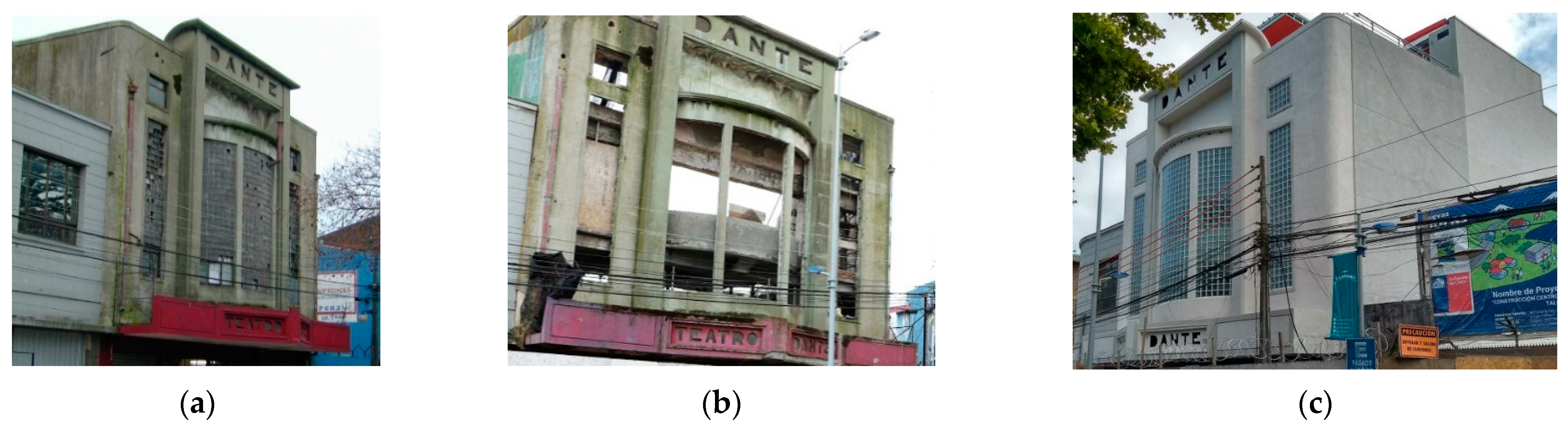
- GD Ingenieros LTDA. Peritaje Estructura Edificio Antiguo Teatro Dante Talcahuano, Sector de Fachada, Hall Acceso y Graderías; Technical Report; Concepcion, Chile, 2012; In Spanish. [Google Scholar]


| Soil Class | Factor A | ||||
|---|---|---|---|---|---|
| Pre 1972 | 1972–1992 | 1993–1995 | 1996–2012 | Post 2012 | |
| A | 0.7 | 1.0 | 0.9 | 1.0 | 1.0 |
| B | 0.7 | 1.0 | 0.8 | 1.0 | 1.0 |
| C | 0.7 | 1.0 | 0.8 | 0.9 | 1.0 |
| D | 0.7 | 1.0 | 0.7 | 0.8 | 1.0 |
| E | 0.7 | 1.0 | 0.7 | 0.8 | 1.0 |
| Damage Type | Description of the Damage | Deterioration Factor |
|---|---|---|
| Total destruction | Implies that the structure suffered a total collapse of beams and columns | 0.10 |
| Irrecoverable damage | Implies that the building is at risk of collapsing. | 0.25 |
| Severe damage | The safety of the building’s residents is at risk. | 0.50 |
| Partial damage | Nonstructural damage to the building (more than slight), recoverable, does not hinder its habitability. | |
| Recoverable damage | Nonstructural damage to doors, windows, glass, nonstructural walls, ceilings; minor damage to plumbing installations, etc. (caused by the catastrophe). | 0.75 |
| No damage | There is no damage that affects functionality. | 1.00 |
| Year | Number Earthquakes | ||||
|---|---|---|---|---|---|
| 0 | 1 | 2 | 3 | 4 | |
| pre 1972 | 1.00 | 0.10 | 0.10 | 0.10 | 0.10 |
| 1972–1992 | 1.00 | 0.25 | 0.10 | 0.10 | 0.10 |
| 1993–1995 | 1.00 | 0.25 | 0.10 | 0.10 | 0.10 |
| 1996–2012 | 1.00 | 0.25 | 0.25 | 0.10 | 0.10 |
| post 2012 | 1.00 | 0.25 | 0.25 | 0.25 | 0.10 |
| Year | Number Earthquakes | ||||
|---|---|---|---|---|---|
| 0 | 1 | 2 | 3 | 4 | |
| pre 1972 | 1.00 | 0.25 | 0.10 | 0.10 | 0.10 |
| 1972–1992 | 1.00 | 0.25 | 0.10 | 0.10 | 0.10 |
| 1993–1995 | 1.00 | 0.50 | 0.25 | 0.10 | 0.10 |
| 1996–2012 | 1.00 | 0.50 | 0.50 | 0.25 | 0.10 |
| post 2012 | 1.00 | 0.50 | 0.50 | 0.25 | 0.25 |
| Year | Number Earthquakes | ||||
|---|---|---|---|---|---|
| 0 | 1 | 2 | 3 | 4 | |
| pre 1972 | 1.00 | 0.25 | 0.10 | 0.10 | 0.10 |
| 1972–1992 | 1.00 | 0.50 | 0.10 | 0.10 | 0.10 |
| 1993–1995 | 1.00 | 0.50 | 0.25 | 0.10 | 0.10 |
| 1996–2012 | 1.00 | 0.75 | 0.50 | 0.25 | 0.10 |
| post 2012 | 1.00 | 0.75 | 0.50 | 0.25 | 0.25 |
| Factor | Structural Characteristics | Effect on Structural Performance | ||
|---|---|---|---|---|
| Severe Factor = 0.4 | Significant Factor = 0.7 | Insignificant Factor = 1.0 | ||
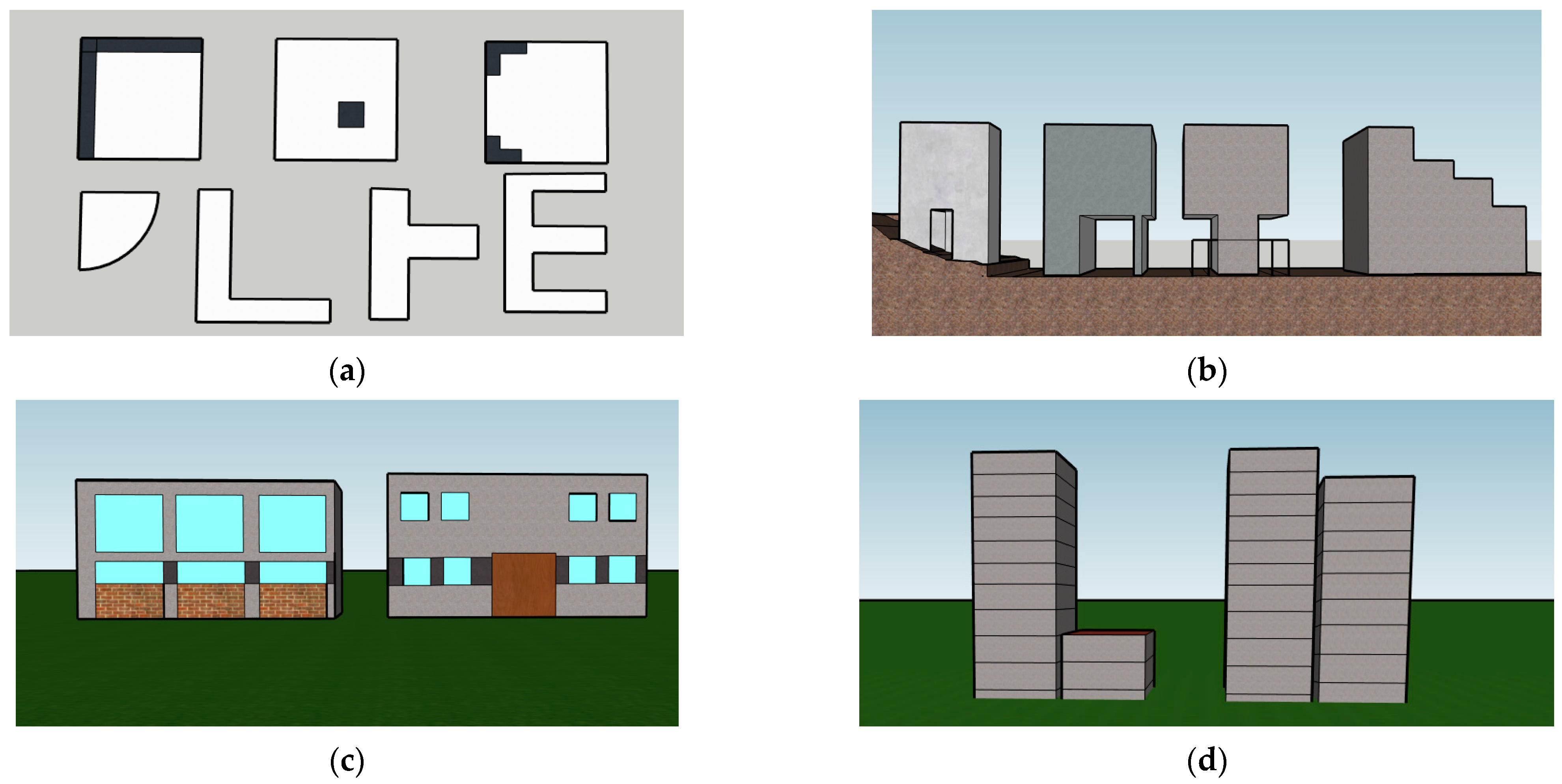
| Factor C | L-shape, T-shape, E-shape | Two or more wings >3.0 in length/width, or one wing >4 in length/width >4 | One wing length/width >3.0 | All wings length/width ≤3.0 |
| Long narrow building where spacing of lateral load resisting elements is: | >4 times building width | >2 times building width | ≤2.0 times building width | |
| Torsion (corner building) | Mass to center of rigidity offset >0.5 width | Mass to center of rigidity offset >0.3 width | Mass to center of rigidity offset ≤0.3 width, or effective torsional resistance available from elements orientated perpendicularly | |
| Ramps, stairs, walls, stiff partitions | Clearly grouped, clearly an influence | Apparent collective influence | No or slight influence | |
| Factor D | Soft story | Lateral stiffness of any story <0.7 of lateral stiffness of any adjoining stories | Lateral stiffness of any story <0.9 of lateral stiffness of the adjoining stories | Lateral stiffness of any story ≥0.9 of lateral stiffness of the adjoining stories |
| Mass variation | Mass of any story <0.7 of mass of adjoining story | Mass of any story <0.9 of mass of adjoining story | Mass of any story ≥0.9 of mass of adjoining story | |
| Vertical discontinuity | Any element contributing >0.3 of the stiffness/strength of the lateral force resisting system discontinues vertically | Any element contributing >0.1 of the stiffness/strength of the lateral force resisting system discontinues vertically | Only elements contributing ≤0.1 of the stiffness/strength of the lateral force resisting systems discontinue vertically | |
| Factor E | Columns <70% story height between floors clear of confining infill, beams or spandrels | Either >80% short columns in any one side, or >80% short columns in any story | >60% short columns in any one side, or >60% columns in any one story | No, or only isolated, short columns, or columns with width >1.2 m, or Free column height/column width ≥2.5. |
| Factor F | F1: Pounding Vertical differences between floors >20% story height of building under consideration | 0 < separation < 0.005 h | 0.005 H < separation < 0.01 h | Separation > 0.01 h |
| F2: Height difference Height difference in 2 to 4 stories | 0 < separation < 0.005 H | 0.005 H < separation < 0.01 H | Separation > 0.01 H | |
| Height difference in more than 4 stories | 0 < separation < 0.005 H | 0.005 H < separation < 0.01 H | Separation >0.01 H, or floors aligning and height difference <2 stories, or at least one building is lightweight construction | |
| %NBS | SVA Rating | Level of Vulnerability |
|---|---|---|
| ≥100 | Very low | |
| 80–99 | Low | |
| 34–79 | Medium | |
| –33 | High | |
| <20 | Very high |
| Variable (Vulnerability Score) | Very Low (1) | Low (2) | Medium (3) | High (4) | Very High (5) | |
|---|---|---|---|---|---|---|
| PV1 | Geomorphology | High cliffs | Medium cliffs | Low cliffs, hills or mountains | Alluvial plains, coastal lagoons | Beach, dune fields |
| PV2 | Average wave height (m) | <0.55 | 0.55–0.85 | 0.85–1.05 | 1.05–1.25 | >1.25 |
| PV3 | Average tidal range (m) | >6 | 4.1–6 | 2–4 | 1–1.9 | <1 |
| PV4 | Beach width (m) | >50 | 50–25 | 25–10 m | <10 | No beach |
| PV5 | Coastal slope (%) | >15 | 15–10 | 10–5 | 5–2 | <2 |
| PV6 | Distance to water body (m) | >557 | 557–417 | 416–196 | 195–66 | <66 |
| PV7 | Coastal protection | Natural | – | Constructed | – | No protection |
| SV1 | Number of stories | Three levels | – | Two levels | – | One level |
| SV2 | State of conservation | Good | – | Regular | – | Bad |
| SV3 | Material | RC | M | RC + T/M + T | T | PB |
| SDV1 | Socioeconomic status | Professional | Technical | Production | Artisan | Agriculture |
| SDV2 | Pop. density (inhab/km2) | <9000 | 9000–20,000 | 20,000–40,000 | 40,000–80,000 | >80,000 |
| Index | Very Low | Low | Medium | High | Very High |
|---|---|---|---|---|---|
| CVIP | <0.28 | 0.28–0.64 | 0.64–1.19 | 1.19–1.92 | 1.92< |
| CVIS | <1.44 | 1.44–2.78 | 2.78–5.26 | 5.26–7.93 | 7.93< |
| CVISD | <1.25 | 1.25–3.25 | 3.25–6.25 | 6.25–10.25 | 10.25< |
| NCVI | 1 | 2 | 3 | 4 | 5 |
| Variable Type | Variable Weights | Variable Type Weights | ||||||
|---|---|---|---|---|---|---|---|---|
| Physical | α1 | α2 | α3 | α4 | α5 | α6 | α7 | wP |
| 0.30 | 0.20 | 0.22 | 0.09 | 0.11 | 0.03 | 0.04 | 0.46 | |
| Structural | β1 | β2 | β3 | – | – | – | – | wS |
| 0.33 | 0.40 | 0.27 | – | – | – | – | 0.29 | |
| Sociodemographic | γ1 | γ2 | – | – | – | – | – | wSD |
| 0.86 | 0.14 | – | – | – | – | – | 0.25 | |
| Distance to Coast (m) | Weights | |
|---|---|---|
| wS | wC | |
| >D | 1.0 | 0 |
| D–D/2 | 0.5 | 0.5 |
| D/2–D/4 | 0.4 | 0.6 |
| <D/4 | 0.3 | 0.7 |
| Vulnerability Assessment | Very Low | Low | Medium | High | Very High |
|---|---|---|---|---|---|
| VA | ≤1.0 | 1.1–2.0 | 2.1–3.0 | 3.1–4.0 | ≥4.1 |
| Factor | A | B | C | D | E | F | G | %NBS | SVA |
|---|---|---|---|---|---|---|---|---|---|
| Pre-2010 | 0.7 | 0.25 | 0.70 | 1.00 | 1.00 | 1.00 | 1.00 | 12.3% | 4.39 |
| Post-2010 | 0.7 | 0.10 | 0.70 | 1.00 | 1.00 | 1.00 | 1.00 | 4.9% | 4.76 |
| Post-2018 | 1.00 | 1.00 | 0.70 | 1.00 | 1.00 | 1.00 | 1.00 | 70.0% | 2.22 |
| Variable | PV1 | PV2 | PV3 | PV4 | PV5 | PV6 | PV7 | SV1 | SV2 | SV3 | SDV1 | SDV2 | CVA |
|---|---|---|---|---|---|---|---|---|---|---|---|---|---|
| Pre-2010 | 5 | 3 | 5 | 3 | 4 | 3 | 3 | 3 | 2 | 2 | 3 | 1 | 3.17 |
| Post-2010 | 5 | 3 | 5 | 3 | 4 | 3 | 3 | 5 | 5 | 2 | 3 | 1 | 3.75 |
| Post-2018 | 5 | 3 | 5 | 3 | 4 | 3 | 3 | 3 | 1 | 1 | 3 | 1 | 2.88 |
| Variable | SVA | CVA | VA | Vulnerability Level |
|---|---|---|---|---|
| Pre-2010 | 4.39 | 3.17 | 3.53 | High |
| Post-2010 | 4.76 | 3.75 | 4.05 | Very High |
| Post-2018 | 2.22 | 2.88 | 2.68 | Medium |
| Building Code | SVA | CVA | VA | Vulnerability |
|---|---|---|---|---|
| EB1 | 4.10 | 2.88 | 3.25 | High |
| EB2 | 1.00 | 2.88 | 2.32 | Medium |
| EB3 | 1.00 | 2.88 | 2.32 | Medium |
| EB4 | 4.10 | 2.88 | 3.25 | High |
| EB5 | 2.65 | 2.88 | 2.81 | Medium |
| EB6 | 2.98 | 2.88 | 2.91 | Medium |
| PuB1 | 1.00 | 2.88 | 2.32 | Medium |
| PuB2 | 1.00 | 2.88 | 2.32 | Medium |
| PuB3 | 4.10 | 2.88 | 3.25 | High |
| PuB4 | 1.00 | 2.88 | 2.32 | Medium |
| PuB5 | 1.00 | 2.88 | 2.32 | Medium |
| PuB6 | 1.00 | 2.88 | 2.32 | Medium |
| PrB1 | 2.43 | 2.88 | 2.75 | Medium |
| PrB2 | 2.43 | 2.88 | 2.75 | Medium |
| CB1 | 1.00 | 2.88 | 2.32 | Medium |
| CB2 | 4.10 | 2.88 | 3.25 | High |
| CB3 | 2.43 | 2.88 | 2.75 | Medium |
| CB4 | 2.43 | 2.88 | 2.75 | Medium |
Publisher’s Note: MDPI stays neutral with regard to jurisdictional claims in published maps and institutional affiliations. |
© 2021 by the authors. Licensee MDPI, Basel, Switzerland. This article is an open access article distributed under the terms and conditions of the Creative Commons Attribution (CC BY) license (http://creativecommons.org/licenses/by/4.0/).
Share and Cite
Quiñones-Bustos, C.; Bull, M.T.; Oyarzo-Vera, C. Seismic and Coastal Vulnerability Assessment Model for Buildings in Chile. Buildings 2021, 11, 107. https://doi.org/10.3390/buildings11030107
Quiñones-Bustos C, Bull MT, Oyarzo-Vera C. Seismic and Coastal Vulnerability Assessment Model for Buildings in Chile. Buildings. 2021; 11(3):107. https://doi.org/10.3390/buildings11030107
Chicago/Turabian StyleQuiñones-Bustos, Catalina, Maria Teresa Bull, and Claudio Oyarzo-Vera. 2021. "Seismic and Coastal Vulnerability Assessment Model for Buildings in Chile" Buildings 11, no. 3: 107. https://doi.org/10.3390/buildings11030107
APA StyleQuiñones-Bustos, C., Bull, M. T., & Oyarzo-Vera, C. (2021). Seismic and Coastal Vulnerability Assessment Model for Buildings in Chile. Buildings, 11(3), 107. https://doi.org/10.3390/buildings11030107