Abstract
Neighborhood characteristics influence natural urban energy fluxes and the choices made by urban actors. This article focuses on the impact of urban density as a neighborhood physical parameter on building energy consumption profiles for seven different metropolitan areas in the United States. Primarily, 30 × 30 m2 cells were classified into five categories of settlement density using the US Geological Survey’s National Land Cover Dataset (NLCD), the US Census, and Census Block data. In the next step, linear hierarchical spatial and non-spatial models were developed and applied to building energy data in those seven metropolitan areas to explore the links between urban density (and other urban form parameters) and energy performance, using both frequentist and Bayesian statistics. Our results indicate that urban density is correlated with energy-use intensity (EUI), but its impact is not similar across different metropolitan areas. The outcomes of our analysis further show that the distance from buildings within which the influence of urban form parameters on EUI is most significant varies by city and negatively changes with urban density. Although the relationship between urban density parameters and EUI varies across cities, tree-cover area, impervious area, and neighborhood building-covered area have a more consistent impact compared to building and housing density.
1. Introduction
Urban areas are hubs of economic, social, and cultural activity and therefore major consumers of energy and producers of greenhouse gas emissions [1]. With the current trends in urbanization and the expected growth of 2.5 billion people in the global urban population between 2018 and 2050, energy demand of cities is expected to increase drastically in the future [2]. In order to meet strategic energy security goals and control climate change, urban communities are putting a lot of emphasis on transitioning to sustainability by cutting their energy consumption. However, considering the scale and pace of the urbanization process, the impact of spatial patterns of urbanization on energy consumption remains largely underexplored.
Cities have different morphologies, and these morphologies are referred to as integrated wholes [3] that can be considered at different levels of resolution. These resolution levels are consonant with various components of urban form [4]. Urban form is identified as the physical qualities of the urban natural and built environment, in terms of size, shape, configuration, and settlement density that foster interactions between people, activities, and geographical spaces [5,6,7]. With regard to energy, urban form impacts both operational and embodied energy in the built environment [8,9]. In addition, the positioning of buildings and urban blocks, land-use mix, street connectivity, and population density patterns can change transport characteristics and the associated mobile sources of energy consumption and carbon emissions [10,11].
The debate over whether compact or dispersed city prototypes better foster urban sustainability has a long history. The advocates for high-density development (e.g., [12,13,14,15]) argue that concentrated urban configurations result in reduced transport energy use, contribute to affordable transportation, create a cleaner environment, improve quality of life and the social mix, and positively impact public health [16,17]. However, it is also argued, in contrast, that compact forms increase impervious surfaces, contributing to a greater urban heat island (UHI) effect; forsake non-urban communities; weaken local decision-making structures; increase congestion; and eliminate urban green spaces [17,18]. Neuman [19] considers compactness to be neither a necessary nor sufficient characteristic of sustainable cities. Holden and Norland [20] believe that taking sides in the compact/dispersed dispute for sustainability enthusiast planners requires two questions answered at the outset: what features of sustainability matter the most, and which urban form yields the highest energy efficiency?
The body of literature on the impact of urban form characteristics on household travel and transportation energy demand is extensive (e.g., [21,22,23,24]). In addition, urban form impacts building energy use through UHI effect and electric transmission and distribution (T&D) losses, also directly through energy requirements of the building stock [25,26]. However, T&D losses in the US average only about 5% of the total annually, suggesting that urban form’s impact on T&D losses is altogether insignificant in magnitude [27]. Overall, in comparison, there is little research on the influence of urban land-use and form on building energy profiles and carbon emissions, beyond the UHI effect.
Despite the limited frequency of form-energy compared to form-transportation studies, urban form has been universally acknowledged as an important parameter in the analysis of building energy performance. Form, through the layout and orientation of urban blocks [28,29], vegetation, and high albedo materials [30,31,32], and the shading effect of the surrounding blocks [33,34], changes the microclimate within building networks. In order to explore the impact of urban configuration on the energy balance of buildings and outdoor climate conditions, Adolphe [35] introduced a simple spatial model using morphological parameters such as density, solar admittance, rugosity, compacity, and contiguity. Using building shape factors, the depth and obstruction angle, Steemers [36] explored the relationship between urban morphology and energy consumption. Ratti et al. [37] applied digital elevation models (DEMs) and used the distance between facades and the urban surface-to-volume ratio to link energy use to urban texture. Krüger et al. [38] report that increased height of adjacent buildings reduces cooling demands, similar to the effect of deeper streets [39]. Strømann-Andersen and Sattrup [40] concluded that urban canyon form can modify energy consumption of low-energy buildings by up to 19% and 30% for residential and office buildings respectively. Wong et al. [41] explored the impact of 32 different urban setting scenarios on the energy performance of a three-story office building in Singapore and demonstrated that the height of the surrounding buildings can potentially reduce air-conditioning energy use by up to 5%. Under modified alternative scenarios, Mills [42] analyzed the energy performance of a building adjacent to a street in the downtown area of London, UK, using thermal dynamic simulation tools and suggested that the impact of urban morphology on annual cooling load can reach up to 12%. Ahn and Sohn [43] explored the impact of building height, density, and compactness on multi-family housing energy use for the city of Seattle using a spatial regression model, and concluded that form factors are more consequential for EUI at close distance ranges.
Although there is no definitive agreement on defining and measuring urban form, concepts of density, concentration, proximity, continuity, and compactness have been helpful across the literature [26,44]. Nonetheless, it is not always easy to exactly delineate such terms with consensus. As an example, defining urban density is still a matter of controversy within the planning community. Some planners use the number of people per square mile as an indicator, and some use the recorded number of vehicles between urban centers. One challenge is that the correlation between these two different measures of density is not even always strong. Güneralp et al. [45], taking urban density as population density, projected residential and commercial floor area per capita using GDP and population growth scenarios and concluded that urban density scenarios can be as effective as efficiency upgrades in reducing heating and cooling energy consumption by 2050. In their study, a negative correlation was reported between urban density and building energy use. However, it is beyond question that, if urban density is defined solely as population density, any increase in density can only result in dwelling size reduction and, consequently, lower energy consumption numbers. Better density indicators that make it possible to bring together population, physical environment, and the generated traffic still need to be defined [46,47].
In this paper, we explored the impact of urban density, as a major indicator of urban form, on building energy use in seven major US metropolitan areas. Our research questions were: (1) What proximity to a building is more relevant to be taken into account when the impact of urban density on energy consumption is of concern? (2) What is the impact of urban density—and other urban form parameters—on building energy use intensity (EUI)?
2. Methodology
2.1. Data
The urban density data for this study were obtained from three different sources that are updated every five to ten years. Housing units’ populations at the Census-Block level were compiled nationwide for 2000 and 2010, providing a high-resolution insight into population and housing information. Housing data and the Census Block polygons were connected using Python and respectively obtained from the US Census Bureau website and Topologically Integrated Geographic Encoding and Referencing (TIGER) GIS data. For stratifying settlement morphologies within which buildings stand, a method developed by Heris [48] was applied that uses a cell-based density profile to assign a general type of urban context to each building’s neighborhood. This method offers a national raster layer in which the settlement type for each cell is defined as high-density urban core, medium density, low density, urban fringe, or suburban. To incorporate building footprints in our model, Microsoft’s building dataset (https://github.com/Microsoft/USBuildingFootprints, accessed on 5 November 2019), which covers the entire US, was used (Figure 1).
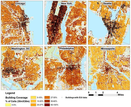
Figure 1.
Building footprint coverage in 30 × 30 m2 cells.
High resolution 1 m2 land-cover datasets available through the EPA’s EnviroAtlas data portal (https://www.epa.gov/enviroatlas/enviroatlas-data-approach, accessed on 25 October 2019) were used to measure the percentage of tree canopy and impervious surface cover for each cell. Surface temperature data for 30 × 30 m2 cells were extracted from Landsat 8 OLI images with less than 1% cloud cover. Atmospheric corrections were applied using ENVI for all bands, including thermal ones, and the Landsat Digital Numbers (DNs) of band 10 were converted to top-of-atmosphere (TOA) reflectance in accordance with USGS instructions (http://landsat.usgs.gov/Landsat8_Using_Product.php, accessed on 20 July 2021):
where . is the TOA spectral radiance (Watts/(m2.srad.μm)), is the band-specific multiplicative rescaling factor from the metadata, is the band-specific additive rescaling factor, and is the quantized and calibrated standard product pixel value (DN). In the next step, radiance values were converted to the satellite brightness temperature:
where T is the at-satellite brightness temperature (K), and K1 and K2 are band-specific thermal conversion constants from the metadata. In the last step, satellite brightness temperature (BT) data were normalized based on emissivity values for each land-cover class using the following equation:
where W is the wavelength of emitted radiance and P = h *c/s (=14,380), with s as the Boltzmann constant, h as the Planck constant, and c as the velocity of light (Figure 2).

Figure 2.
Surface temperature distribution (1 m2 resolution).
Energy data were collected for the cities of interest from different sources depending on the city-specific reporting requirements of energy benchmarking initiatives (mostly based on building type and size). For instance, Seattle’s Energy Benchmarking Program (SMC 22.920) mandates that the annual energy performance for non-residential and multifamily buildings over 1858 m2 (20,000 ft2) be reported by owners to the city (see Table 1 for the building-type mix by city). Every building data-point that carried energy-use data was geocoded based on longitude and latitude. All the above-mentioned layer sections were converted to raster layers at 30 × 30 m2 resolution. For land-cover layers, tree canopy and impervious surface coverage information were aggregated from 1 × 1 m2 to 30 × 30 m2 resolutions.

Table 1.
Summary of building-type shares in different cities’ datasets.
It shall be noted that some data processing was done prior to the analysis in order to connect the datasets. First, Census Block polygons of different years are not identical. Second, in core urban areas, Census Blocks are small and most of their net areas are developed. To reach a normalized building density measure and deal with the problem of having lower housing or population densities in low-resolution areas, it was necessary to identify the built sites and exclude open spaces. This was done using the NLCD product ‘percent developed imperviousness’ to exclude land that was entirely undeveloped, particularly in suburban communities. However, the presence of roads as impervious surfaces in these areas created significant noise in the data. After comparing different road network datasets such as TIGER lines and Open Street Map (OSM), OSM data were chosen for the analysis since they exclude roads from the impervious surface measurement.
2.2. Analysis
The two major tasks on hand were to identify the distance from a particular building at which it is most relevant to study the impact of urban form parameters on building energy use and to determine the relationship between form parameters and energy consumption. To answer the first question and to create an inquiry into variables for different distances from a particular building, our algorithm ran the explained script for windows of different sizes. These hypothetical windows were in the shape of squares (to match the 30 m × 30 m analysis units) drawn around every single building point and covering areas amounting to 150 × 150, 270 × 270, 390 × 390, …, 1950 × 1950 m2. For every window, urban form composites were created using a principal component analysis (PCA) in which correlated variables were loaded into orthogonal components. The variables used to create each of the composites were the average area of the buildings, number of buildings per hectare, average tree-cover area, impervious surface area, morphological density category (1–5; 1 = low density, 5 = high density), number of housing units per hectare, and surface temperature for all of the windows. It is important to note that, ultimately, only the first three components in each PCA were technically used in evaluating the relationship between urban form and EUI (energy per area per year) since 80% or more of the variance in all windows for all the cities was explained by them.
A stepwise regression analysis of EUI, log-transformed to correct for its non-normality, was then carried out on a series of covariates and the urban form composites. Using the Akaike information criteria (AIC), an estimator of the relative quality of statistical models, the additional variance explained by adding the urban form composites to each model was observed for each window. Two requirements had to be met in selecting the optimal window: the urban form composite needed to impact the model’s R2 significantly, and the additional predictive power was supposed to be the greatest of all the windows in which the first requirement was met.
As Table 2 shows, in six out of the seven cities the considered urban form parameters did show an impact on energy consumption patterns. In the case of Minneapolis, MN, the small data size could have been the reason behind no clear pattern emerging. The results are as interesting as they are intuitive: in cities with more sprawled agglomerations like Austin, TX, the impact of variables such as surface temperature, average area of the buildings, number of buildings per hectare, average tree-cover area, and impervious surface area within the 1.5 km radius better explains the impact of urban form on building energy. However, in cities with higher urban densities the impact of the mentioned variables on EUI was most relevant in the immediate 0.5 km radius around the buildings.
Table 2.
Significance of urban form variables’ impact on energy consumption.
The second research question concerned determining the relationship between urban density parameters and building energy consumption. Regression models of the EUI on a set of relevant covariates and urban form variables were fitted for the optimal window for each city, selected in the previous stage. However, the urban form composites were not applied at this stage, since using the original variables would have provided a better perspective for interpreting the relationships between form parameters and EUI. Also, surface temperature was absent in some of the final models since it could be modelled as a function of tree-cover area and impervious surface area, and it did not always add relevant variance to the models. The dependent variable was the log-transformed version of the EUI. The model predictors were selected using a stepwise approach and linear ordinary least square (OLS) models. All models were checked for multicollinearity to avoid correlated urban form variables inflating the variance explained by the models. In cases with the presence of multicollinearity, certain variables were excluded until normal levels of the variance inflator factor (VIF) were reached (below 4). The selection of covariates for each model was strongly determined by data availability and model predictive power. There were some discrepancies in the variables incorporated in the city-specific models since the energy data came from different sources.
The resulting models were also evaluated for spatial dependency by analyzing the residuals using graphical and statistical methods; namely, Moran’s I [49], which is a measure of overall spatial autocorrelation. To run the Moran statistic and the spatial regression models, matrices of neighbors were created in which, for the sake of consistency across the models, the 20 closest units in the dataset (according to their GPS coordinates) were defined as neighbors of each unit. Since this approach could yield asymmetrical matrices of neighbors [50], the matrices were corrected to make them symmetric; therefore, some units ended up having more than 20 neighbors in the last iteration. Finally, the matrices were weighted based on the inverse distance between the different units in order to acknowledge the higher influence of the closer neighbors. Moran’s I can be explained as:
where is an element of the row-standardized weights matrix W, and is the value of the variable under examination (for instance, a residual or a dependent variable) for observation i. Moran’s I was applied to determine whether EUI should be modelled using spatial regression methods (as opposed to non-spatial). As Moran’s I is sensitive to spatial patterning, for robustness, we replicated the calculations using Monte-Carlo simulations of the index (Monte-Carlo replications were consistent with the original index in every single case; see Chen [51] for a more nuanced discussion on this topic). Among the broad range of spatial modeling techniques, the spatial error model (SEM) method was chosen:
where is the independent error term (it is assumed that ), is the connectivity matrix, is the spatial error parameter, and is the spatial component of the error term. SEMs assume that the remaining spatial dependency, not represented by the model variables, exists thanks to a set of unknown spatial factors, as opposed to a form of interaction between the included variables and space [49]. Therefore, applying the SEM framework is more theoretically justifiable since the assumption is that the energy consumption of a unit is not directly impacted by that of its neighbors, and any spatial correlation is more likely due to unobserved variables. Neighbors are unlikely to share energy consumption data among themselves, and parameters such as the property value or urban form variable incorporate the possible existing correlations with space.
As a last step, some of the models were replicated using a Bayesian framework to enable further exploration and disentanglement of more intricate forms of nesting by fitting hierarchical spatial models. To fit these models, the brms package in R was used with standard priors [52]. Brms provides a unified framework to model multilevel spatial regression, is easy to use, and allows users to access all the merits of the Stan program. Stan is a high-level language in which the user specifies a model and the starting values, and then a Hamiltonian Monte-Carlo (HMC) chain simulation is implemented to derive the posterior distributions. These methods converge faster than the more commonly used Metropolis–Hastings algorithm and/or Gibbs sampling, especially for high-dimensional modes [53]. While using HMC may extend the time needed to calculate the gradient of the log-posterior, it provides higher quality samples than other samplers and enables drawing samples from the posterior predictive distribution as well as the pointwise log likelihood [53]. Model fit was assessed by calculating the widely applicable information criterion (WAIC) and the leave-one-out cross-validation method (LOO), both available in brms. To perform the calculations, Proteus, a high-performance shared computer cluster of Drexel University’s Research Computing Facilities, was used. All models implemented in brms are distributional models, where a response “y” is estimated through the prediction of the parameters “θ” of a distribution response “D”.
In turn, each parameter of the distribution response may be regressed on its own predictor term . While can take non-linear forms, it is typically written as a linear combination of population-level effects (X), group-level effects (Z), and smooth functions (sk) fitted via splines as follows:
Prior distributions can be specified in brms or can be used at their default. For example, the default priors for a Gaussian distribution are flat priors for the betas and a t distribution with three degrees of freedom for sigmas; priors for the spatial error parameter are flat priors over [0,1]. With regard to hierarchical Bayesian models, brms builds upon the syntax of other R packages and allows users to model hierarchical relationships for the predictors and/or response function “y”.
3. Regression Results
3.1. City-Specific Trends
To choose whether to fit a linear, linear hierarchical, or spatial model (linear), the Moran’s I for the residuals of the corresponding non-spatial models was examined. The outcome suggested spatial models for all cities except Washington DC (Table 3).
Table 3.
Moran’s I for different cities.
The Washington DC model was hierarchical, non-spatial, and included building type/age/area, property value, the interaction between area and age, and some of the urban form variables for the 1950 × 1950 m2 window. Building type and urban form parameters were the major determinants of energy consumption in DC. Residential units, on average, had a lower EUI (by 18.09%) than non-residential units. The morphological density category was negatively correlated with EUI, with units located in high-density urban-core areas consuming 7.39% less than units located in medium-density areas. Finally, despite statistical significance, the impact of building coverage in the surroundings on EUI was not greater than 0.001%.
The final Austin, TX regression model was spatial and included building type, property value, percentage of residential neighbors, and the urban form variables for the 1950 × 1950 m2 window. Some of the spatial form variables were removed due to multicollinearity. The only form variable significantly associated with energy consumption was the tree cover area in the case of Austin, with each square meter increase in tree cover associated with a 0.2% rise in EUI.
In the case of Chicago, IL, 40% of the total 1707 units in the dataset were residential. The selected model was spatial and included building type/area, percentage of residential neighbors, property value, building age, and the urban form variables for the 270 × 270 m2 window. Building type and building count per hectare were significantly related to energy consumption. Residential units consumed on average 6.74% less energy than non-residential units. Furthermore, building count per hectare was negatively related to EUI. Each extra building was associated with a 0.14% reduction in EUI, indicating a slight negative correlation between density and EUI. Building age and the area covered by buildings were also significantly correlated with energy consumption, although negligible in magnitude.
The final New York City model was spatial and included building type/age/area, percentage of residential neighbors, property value, and the form variables for the 390 × 390 m2 window. Impervious area and residential density around a building were positively associated with energy consumption intensity. One square meter increase in impervious area was associated with 0.06% higher EUI. In addition, every 10% increase in the proportion of residential neighbors was associated with a 1.59% rise in energy consumption.
The Philadelphia, PA model was also spatial and included building type/age/area, percentage of residential neighbors, property value, and the urban form variables for the 510 × 510 m2 window. In Philadelphia, every unit of increase in building area was associated with a 10.87% rise in EUI. Also, the building count per hectare had a positive relation with energy use, with each added building leading to an increase in EUI by 2.38%.
The selected regression model for Seattle was spatial and included building type/age/area, property value, the percentage of residential neighbors, and urban form factors for the 1590 × 1590 m2 window. The results showed lower consumption for residential units by 33.29% and, like the other cases, positive correlation between area and EUI. One unit of increase in building count per hectare led to a 1.63% increase in energy consumption, while the morphological density variable positively correlated with energy-consumption intensity. The area of units was treated as a categorical variable, with 10 categories each representing 10% of the sample. The results showed that a unit jump in unit area was associated with a 1.91% increase in EUI. One unit increase in building count per hectare was associated with an energy consumption reduction of 1.14%. Furthermore, a unit increase in the morphological density category was associated with an increase in energy-consumption intensity by 19.15%. A summary of the results for all the cities is provided in Table 4.
Table 4.
A summary of the impacts of urban form and density variables on energy-use intensity (gray = positive correlation; white = negative correlation; numbers provided only for the statistically significant relationships).
The spatial error parameter was positive and significantly different from zero in all the spatial models, indicating a positive spatial dependency between the estimates and hinting at the existence of spatial factors that impact EUI that were not accounted for by other parameters in the models.
3.2. Cities Combined
While not all the city-specific datasets provided information on the exact same set of parameters, there was some overlap that enabled running a model across the cities. The first step was to select a spatial window. The 510 × 510 m2 window was chosen for its higher predictive power, based on the method previously introduced for the city-specific models. The morphological density category needed to be transformed into a dichotomous variable to recognize that most of the units in the dataset came from highly dense neighborhoods. Furthermore, the types of units included in the model were reconsidered to incorporate categories that represented at least 2% of the total units in the combined dataset, giving relevance to categories such as hospitals or worship centers. Lastly, some variables were dropped due to multicollinearity.
Most of the variables in the model were relevant in predicting the EUI (Table 5). The results suggest that residential units, warehouses, and worship centers consume, on average, less energy than other unit types (15.42%, 59.34%, and 36.90% less, respectively), while hotels and hospitals consume more (39.26% and 138.81% more, respectively). Beyond the unit type, there were other variables that explained the differences in EUI. For instance, units in NYC and Chicago tended to have higher EUIs than DC units, with everything else constant. Four of the urban form variables reached the statistical significance level: a 1 m2 increase in tree-cover area was associated with an increase in EUI of 0.04%; a 1 m2 increase in impervious area was associated with a 0.02% increase in EUI; a one unit increase in the building count per hectare was associated with a 0.52% reduction in EUI; and, finally, a unit increase in the housing density per hectare was associated with a rise in energy consumption of 0.05%. Cooling degree days (CDD) was also significantly and positively correlated with energy use (0.02% EUI increase per CDD). The spatial error parameter was positive and significantly different from zero ( = 0.281, p-value < 0.001).
Table 5.
Spatial regression results for cities combined.
3.3. The Bayesian Models
Bayesian statistics could offer more insight into the nature of the regression parameters and the relationship between urban form and EUI. The results across cities showed that some of the relationships were less consistent than others, including the relationship between the morphological density category and EUI. This could have been a result of using different spatial windows in different cities or, alternatively, could be attributed to different relationships between the morphological density category and EUI in different cities. In order to gain more insight into this relationship, Bayesian statistics were used. In particular, using a Bayesian framework enabled replication of the combined model and obtaining posterior distributions for the parameters of interest, particularly the coefficient for the morphological density category (Figure 3), allowing a better understanding of these relationships. Due to imperfect convergence, the results should be interpreted with some caution (despite using four chains, the was greater than 1.05 for all parameters, indicating imperfect convergence).
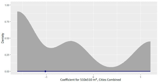
Figure 3.
Distribution of the regression coefficient for the impact of morphological density on EUI (posterior, all cities).
To fully understand the nature of morphological density category, a simpler model was fitted in which units were nested in cities and the morphological density category was added as the only independent variable, yielding higher likelihood of convergence. To capture the full nuances in the relationship, the original variable for the morphological density category (ranging from 0–5) was used, as opposed to the dummy version of it, which was used in the previous models. As shown in Table 6, across cities and in the absence of covariates other than a random error by city, each level of increase in the morphological density category (moving from lower to higher density) was significantly associated with an increase in EUI of 5.13%.
Table 6.
Population level effects: the simplified Bayesian hierarchical spatial model.
The values fell within an acceptable range, indicating that the results could be interpreted with confidence. The results indicate that in the absence of other variables, units in denser areas have on average 5% higher energy consumption. Furthermore, the coefficient associated with the morphological density category was negatively skewed and relatively flat between 0.045 and 0.055, suggesting that the effect should be interpreted as a range more than a single value. Based on this, an increase in morphological density was associated with a 5–6% increase in energy consumption.
Altogether, these results suggest that a correlation between morphological density and EUI does in fact exist but is somehow moderated by the presence of other covariates in a way that is not consistent across different cities. Indeed, Bayesian hierarchical spatial models in each city (obtained on the same models presented before) indicated a case-by-case nature for the relationship between morphological density and energy consumption (Figure 4).
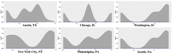
Figure 4.
Posterior distribution of the impacts of morphological density on EUI by city.
4. Conclusions
This paper describes methods for evaluating the impacts of urban density on building energy performance across different metropolitan areas. We analyzed energy data for 12,700 buildings and their urban density conditions across the United States. The buildings were associated with five different morphology density categories (high, medium, and low density, suburban, and urban fringe). Spatial regression methods were applied to explore correlations between building energy-use intensity (EUI) and urban form and physical predictor variables, including impervious area, surface temperature, and tree-cover area around the buildings. Geographical coordinate information were used to define proximity-based neighbors for the spatial regression models. Our goal was to answer two specific questions: (1) What distance from a building is more relevant to be taken into account when the impact of urban density on energy consumption is of concern? (2) What is the relationship between urban density—and other urban form parameters—and building energy-use intensity (EUI)?
Our results suggest that in cities with more dispersed agglomerations, such as Austin, the morphology within the 1.5 km radius better reflects the impact of urban form on building energy use. On the other hand, in cities with denser agglomerations, the impact of density on EUI is most significant for the immediate 0.5 km radius around a given building. The results also indicate that urban density and form do have explanatory potential for EUI; however, the relationship between urban form/density parameters and EUI varies across cities. Among different parameters, the impacts of the tree-cover area, impervious area, and building footprint area in the surroundings on EUI were more consistent across the studied cities compared to the impacts of building count per hectare, housing density per hectare, and the morphological density category. The Bayesian framework applied further suggests that the correlation between morphological density and EUI can, in fact, be moderated by the presence of other covariates and is not consistent across different cities. The Bayesian hierarchical spatial models for each city indicated that the relationship between morphological density and energy consumption could be different in nature across different cities in a way that is not captured by the models.
This study emphasizes the importance of energy-efficient urban planning and building design procedures in accounting for the urban grid structure and the distribution of buildings within that structure. To reach higher energy-efficiency levels, a wider range of interdependencies needs to be incorporated into the planning and design procedure at different scales, from the block to the entire city level. Single element optimization methods that are commonly used commercially usually include a small number of parameters and either concentrate on buildings without taking these interdependencies into consideration or work at metropolitan scales with very large grids that oversimplify the modeling process.
This work presents a methodical approach to disaggregating the impact of vegetation, surface temperature, and urban density for a more nuanced environmental energy analysis. The models, of course, have some limitations. Air and energy flows around buildings are modified by urban morphology and the exchanges between many different exposed surfaces. Tracking these interactions is not a straightforward task. Aerial imagery has improved UHI analysis frameworks. However, the real three-dimensional situation, including buildings’ exterior walls and the urban canopy is much more complex and difficult to capture than the two-dimensional heat gradient for the urban surface. Some factors, such as building height, were not included in our analysis. Furthermore, it would have been potentially more insightful to break down the analysis into monthly intervals, which was not done due to data limitations. Summer and winter periods and the monthly length of daylight time modify heating and cooling energy demand as well as inter-building effects. In other words, the impact of urban layout on energy use may not be consistent throughout the year depending on climate conditions and geographic location. A monthly analysis could provide a thorough perspective on both favorable and detrimental impacts of UHI effects and urban form on energy consumption patterns all year round and enable the creation of more detailed measures to reduce unfavorable urban form-related effects.
The extent to which urban layout impacts the energy performance of the built stock and the importance of considering urban form efficiency in the conception stages of urban projects’ planning must be underscored. Enhanced building stock datasets are necessary to provide further insight into patterns of energy consumption and saving opportunities, especially for growing cities where rapid urbanization accelerates the importance of urban form in the planning process.
Author Contributions
Conceptualization, N.M. and M.P.H.; methodology, N.M., M.P.H. and F.G.; software, N.M., M.P.H. and F.G.; validation, M.P.H., F.G. and S.H.; formal analysis, N.M., M.P.H. and F.G.; resources, S.H.; data curation, N.M., M.P.H.; writing—original draft preparation, N.M., M.P.H.; writing—review and editing, F.G., S.H.; visualization, M.P.H., F.G.; supervision, N.M. and S.H.; funding acquisition, S.H. All authors have read and agreed to the published version of the manuscript.
Funding
This research was partially funded by the National Science Foundation, grant number 1740449.
Institutional Review Board Statement
Not applicable.
Informed Consent Statement
Not applicable.
Data Availability Statement
The data presented in this study are available on request from the corresponding author.
Conflicts of Interest
The authors declare no conflict of interest.
References
- Mostafavi, N.; Farzinmoghadam, M.; Hoque, S.; Weil, B. Integrated Urban Metabolism Analysis Tool (IUMAT). Urban Policy Res. 2014, 32, 53–69. [Google Scholar] [CrossRef]
- United Nations Population Division World Urbanization Prospects: The 2018 Revision. Available online: https://esa.un.org/unpd/wup/ (accessed on 19 July 2018).
- Kropf, K. Urban Tissue and the Character of Towns. Urban Des. Int. 1996, 1, 247–263. [Google Scholar] [CrossRef]
- Oliveira, V. The elements of urban form. In Urban Morphology; Springer: Cham, Switzerland, 2016; pp. 7–30. [Google Scholar]
- Rode, P.; Floater, G.; Thomopoulos, N.; Docherty, J.; Schwinger, P.; Mahendra, A.; Fang, W. Accessibility in Cities: Transport and Urban Form. In Disrupting Mobility: Impacts of Sharing Economy and Innovative Transportation on Cities; Meyer, G., Shaheen, S., Eds.; Lecture Notes in Mobility; Springer International Publishing: Cham, Switzerland, 2017; pp. 239–273. ISBN 978-3-319-51602-8. [Google Scholar]
- Bramley, G.; Power, S. Urban Form and Social Sustainability: The Role of Density and Housing Type. Environ. Plann. B Plann. Des. 2009, 36, 30–48. [Google Scholar] [CrossRef]
- Frank, L.D.; Engelke, P.O. The Built Environment and Human Activity Patterns: Exploring the Impacts of Urban Form on Public Health. J. Plan. Lit. 2001, 16, 202–218. [Google Scholar] [CrossRef]
- Larson, W.; Zhao, W. Telework: Urban Form, Energy Consumption, and Greenhouse Gas Implications. Econ. Inq. 2017, 55, 714–735. [Google Scholar] [CrossRef]
- Rickwood, P.; Glazebrook, G.; Searle, G. Urban Structure and Energy—A Review. Urban Policy Res. 2008, 26, 57–81. [Google Scholar] [CrossRef] [Green Version]
- Wang, S.; Liu, X.; Zhou, C.; Hu, J.; Ou, J. Examining the Impacts of Socioeconomic Factors, Urban Form, and Transportation Networks on CO2 Emissions in China’s Megacities. Appl. Energy 2017, 185, 189–200. [Google Scholar] [CrossRef]
- Crane, R. The Influence of Urban Form on Travel: An Interpretive Review. J. Plan. Lit. 2000, 15, 3–23. [Google Scholar] [CrossRef]
- Burton, E. The Potential of the Compact City for Promoting Social Equity. Achiev. Sustain. Urban Form 2000, 19–29. [Google Scholar]
- Dieleman, F.; Wegener, M. Compact City and Urban Sprawl. Built Environ. 2004, 30, 308–323. [Google Scholar] [CrossRef] [Green Version]
- Yamagata, Y.; Seya, H. Simulating a Future Smart City: An Integrated Land Use-Energy Model. Appl. Energy 2013, 112, 1466–1474. [Google Scholar] [CrossRef]
- Pili, S.; Grigoriadis, E.; Carlucci, M.; Clemente, M.; Salvati, L. Towards Sustainable Growth? A Multi-Criteria Assessment of (Changing) Urban Forms. Ecol. Indic. 2017, 76, 71–80. [Google Scholar] [CrossRef]
- Stevenson, M.; Thompson, J.; de Sá, T.H.; Ewing, R.; Mohan, D.; McClure, R.; Roberts, I.; Tiwari, G.; Giles-Corti, B.; Sun, X.; et al. Land Use, Transport, and Population Health: Estimating the Health Benefits of Compact Cities. Lancet 2016, 388, 2925–2935. [Google Scholar] [CrossRef] [Green Version]
- Frey, H. Designing the City: Towards a More Sustainable Urban Form; Taylor & Francis: Milton Park, Abington, 2003. [Google Scholar]
- Wolsink, M. ‘Sustainable City’ Requires ‘Recognition’—The Example of Environmental Education under Pressure from the Compact City. Land Use Policy 2016, 52, 174–180. [Google Scholar] [CrossRef]
- Neuman, M. The Compact City Fallacy. J. Plan. Educ. Res. 2005, 25, 11–26. [Google Scholar] [CrossRef]
- Holden, E.; Norland, I.T. Three Challenges for the Compact City as a Sustainable Urban Form: Household Consumption of Energy and Transport in Eight Residential Areas in the Greater Oslo Region. Urban Stud. 2005, 42, 2145–2166. [Google Scholar] [CrossRef]
- Kaza, N. Urban Form and Transportation Energy Consumption. Energy Policy 2020, 136, 111049. [Google Scholar] [CrossRef]
- Liu, C.; Shen, Q. An Empirical Analysis of the Influence of Urban Form on Household Travel and Energy Consumption. Comput. Environ. Urban Syst. 2011, 35, 347–357. [Google Scholar] [CrossRef]
- Mindali, O.; Raveh, A.; Salomon, I. Urban Density and Energy Consumption: A New Look at Old Statistics. Transp. Res. Part A Policy Pract. 2004, 38, 143–162. [Google Scholar] [CrossRef]
- Næss, P. Residential Location Affects Travel Behavior—but How and Why? The Case of Copenhagen Metropolitan Area. Prog. Plan. 2005, 2, 167–257. [Google Scholar] [CrossRef]
- Yang, X.; Peng, L.L.H.; Jiang, Z.; Chen, Y.; Yao, L.; He, Y.; Xu, T. Impact of Urban Heat Island on Energy Demand in Buildings: Local Climate Zones in Nanjing. Appl. Energy 2020, 260, 114279. [Google Scholar] [CrossRef]
- Ewing, R.; Rong, F. The Impact of Urban Form on U.S. Residential Energy Use. Hous. Policy Debate 2008, 19, 1–30. [Google Scholar] [CrossRef]
- Wang, M.; Elgowainy, A.; Benavides, P.T.; Burnham, A.; Cai, H.; Dai, Q.; Hawkins, T.R.; Kelly, J.C.; Kwon, H.; Lee, D.-Y.; et al. Argonne GREET Publication: Summary of Expansions and Updates in GREET® 2018; Sysetms Assessment Group, Energy Systems Division; Argonne National Laboratory: Argonne, IL, USA, 2018; p. 32.
- O’Malley, C.; Piroozfarb, P.A.; Farr, E.R.; Gates, J. An Investigation into Minimizing Urban Heat Island (UHI) Effects: A UK Perspective. Energy Procedia 2014, 62, 72–80. [Google Scholar] [CrossRef] [Green Version]
- Valladares-Rendón, L.G.; Schmid, G.; Lo, S.-L. Review on Energy Savings by Solar Control Techniques and Optimal Building Orientation for the Strategic Placement of Façade Shading Systems. Energy Build. 2017, 140, 458–479. [Google Scholar] [CrossRef]
- Gros, A.; Bozonnet, E.; Inard, C. Cool Materials Impact at District Scale—Coupling Building Energy and Microclimate Models. Sustain. Cities Soc. 2014, 13, 254–266. [Google Scholar] [CrossRef]
- Roman, K.K.; O’Brien, T.; Alvey, J.B.; Woo, O. Simulating the Effects of Cool Roof and PCM (Phase Change Materials) Based Roof to Mitigate UHI (Urban Heat Island) in Prominent US Cities. Energy 2016, 96, 103–117. [Google Scholar] [CrossRef]
- Lee, H.; Mayer, H.; Chen, L. Contribution of Trees and Grasslands to the Mitigation of Human Heat Stress in a Residential District of Freiburg, Southwest Germany. Landsc. Urban Plan. 2016, 148, 37–50. [Google Scholar] [CrossRef]
- Pisello, A.L.; Taylor, J.E.; Xu, X.; Cotana, F. Inter-Building Effect: Simulating the Impact of a Network of Buildings on the Accuracy of Building Energy Performance Predictions. Build. Environ. 2012, 58, 37–45. [Google Scholar] [CrossRef]
- Han, Y.; Taylor, J.E.; Pisello, A.L. Exploring Mutual Shading and Mutual Reflection Inter-Building Effects on Building Energy Performance. Appl. Energy 2017, 185, 1556–1564. [Google Scholar] [CrossRef] [Green Version]
- Adolphe, L. A Simplified Model of Urban Morphology: Application to an Analysis of the Environmental Performance of Cities. Environ. Plann. B Plann. Des. 2001, 28, 183–200. [Google Scholar] [CrossRef]
- Steemers, K. Energy and the City: Density, Buildings and Transport. Energy Build. 2003, 35, 3–14. [Google Scholar] [CrossRef]
- Ratti, C.; Baker, N.; Steemers, K. Energy Consumption and Urban Texture. Energy Build. 2005, 37, 762–776. [Google Scholar] [CrossRef]
- Krüger, E.; Pearlmutter, D.; Rasia, F. Evaluating the Impact of Canyon Geometry and Orientation on Cooling Loads in a High-Mass Building in a Hot Dry Environment. Appl. Energy 2010, 87, 2068–2078. [Google Scholar] [CrossRef]
- Ali-Toudert, F. Energy Efficiency of Urban Buildings: Significance of Urban Geometry, Building Construction and Climate Conditions. In Proceedings of the Seventh International Conference on Urban Climate, Yokohama, Japan, 29 June–3 July 2009; Volume 29. [Google Scholar]
- Strømann-Andersen, J.; Sattrup, P.A. The Urban Canyon and Building Energy Use: Urban Density versus Daylight and Passive Solar Gains. Energy Build. 2011, 43, 2011–2020. [Google Scholar] [CrossRef]
- Wong, N.H.; Jusuf, S.K.; Syafii, N.I.; Chen, Y.; Hajadi, N.; Sathyanarayanan, H.; Manickavasagam, Y.V. Evaluation of the Impact of the Surrounding Urban Morphology on Building Energy Consumption. Sol. Energy 2011, 85, 57–71. [Google Scholar] [CrossRef]
- Futcher, J.A.; Mills, G. The Role of Urban Form as an Energy Management Parameter. Energy Policy 2013, 53, 218–228. [Google Scholar] [CrossRef]
- Ahn, Y.; Sohn, D.-W. The Effect of Neighbourhood-Level Urban Form on Residential Building Energy Use: A GIS-Based Model Using Building Energy Benchmarking Data in Seattle. Energy Build. 2019, 196, 124–133. [Google Scholar] [CrossRef]
- Williams, K. Spatial Planning, Urban Form and Sustainable Transport; Routledge: Milton Park, Abingdon, 2017; ISBN 978-1-351-89872-0. [Google Scholar]
- Güneralp, B.; Zhou, Y.; Ürge-Vorsatz, D.; Gupta, M.; Yu, S.; Patel, P.L.; Fragkias, M.; Li, X.; Seto, K.C. Global Scenarios of Urban Density and Its Impacts on Building Energy Use through 2050. Proc. Natl. Acad. Sci. USA 2017, 114, 8945–8950. [Google Scholar] [CrossRef] [Green Version]
- Aschwanden, G.D.P.A.; Haegler, S.; Bosché, F.; Van Gool, L.; Schmitt, G. Empiric Design Evaluation in Urban Planning. Autom. Constr. 2011, 20, 299–310. [Google Scholar] [CrossRef]
- Raimbault, J.; Perret, J. Generating Urban Morphologies at Large Scales; MIT Press: Cambridge, MA, USA, 2019; pp. 179–186. [Google Scholar]
- Heris, M.P. Evaluating Metropolitan Spatial Development: A Method for Identifying Settlement Types and Depicting Growth Patterns. Reg. Stud. Reg. Sci. 2017, 4, 7–25. [Google Scholar] [CrossRef] [Green Version]
- Ward, M.D.; Gleditsch, K.S. Spatial Regression Models; SAGE Publications: Thousand Oaks, CA, USA, 2018; ISBN 978-1-5443-2882-9. [Google Scholar]
- Bivand, R.S.; Pebesma, E.J.; Gómez-Rubio, V.; Pebesma, E.J. Applied Spatial Data Analysis with R, 2nd ed.; Springer: New York, NY, USA, 2013; Volume 747248717. [Google Scholar]
- Chen, Y. Spatial Autocorrelation Approaches to Testing Residuals from Least Squares Regression. PLoS ONE 2016, 11, e0146865. [Google Scholar] [CrossRef] [PubMed] [Green Version]
- CRAN Brms: Bayesian Regression Models Using ‘Stan’. J. Intell. 2020, 8, 5.
- Bürkner, P.-C. Advanced Bayesian Multilevel Modeling with the R Package Brms. R. J. 2018, 10, 395–411. [Google Scholar] [CrossRef]
Publisher’s Note: MDPI stays neutral with regard to jurisdictional claims in published maps and institutional affiliations. |
© 2021 by the authors. Licensee MDPI, Basel, Switzerland. This article is an open access article distributed under the terms and conditions of the Creative Commons Attribution (CC BY) license (https://creativecommons.org/licenses/by/4.0/).