Article

Moisture Redistribution in Full-Scale Wood-Frame Wall Assemblies: Measurements and Engineering Approximation

by
Charles R. Boardman
*,
Samuel V. Glass
and
Samuel L. Zelinka
Building and Fire Sciences, US Forest Service Forest Products Laboratory, Madison, WI 53726, USA
*
Author to whom correspondence should be addressed.
Buildings 2020, 10(8), 141; https://doi.org/10.3390/buildings10080141
Submission received: 14 July 2020 / Revised: 11 August 2020 / Accepted: 11 August 2020 / Published: 14 August 2020
(This article belongs to the Section Building Energy, Physics, Environment, and Systems)

Abstract

:
A counter-balanced mass measurement system was constructed to allow measurement of water loss from a full-scale wood-framed wall assembly. Water was injected onto a localized area of paper towel adjacent to the oriented strand board (OSB) wall sheathing. Moisture pins in the OSB and relative humidity/temperature sensors inside the insulated wall cavity monitored conditions as the wall dried out. The wetted OSB area’s moisture content dropped at a faster rate than the total mass of the wall, indicating moisture redistribution within the wall. A simple model was used to calculate overall moisture redistribution, which was characterized using a near-exponential decay function. This simplification of the inherently three-dimensional physics of moisture redistribution could be incorporated into the one-dimensional hygrothermal models often used in research and engineering practice.

1. Introduction

Long-term moisture durability of exterior wall assemblies is a design requirement. Improper design can lead to problems with moisture accumulation and subsequent degradation of materials, which defeat the primary purposes of any exterior wall. Moisture control strategies for exterior wall assemblies are well known [1]. Recommendations for vapor diffusion control depend on climate and materials of construction, and there are no simple guidelines that apply in every situation [2,3]. A significant goal, no matter the source of the water, is for wall assemblies to have the ability to dry out if they get wet, either during construction or during their service life [4,5]. Drying potential, which is this ability to dry out, is often a concern for wall assemblies that are insulated and air-sealed to levels required by current model energy codes [6,7]. Although considerable research has been conducted on wood-frame walls, further work is still needed in order to provide a quantitative basis to minimize the risk of moisture damage and quantify drying potential.
Oriented strand board (OSB) is commonly used in North American above-grade wall assemblies as a structural sheathing material. Moisture pins that measure electrical resistance through a medium are often used to monitor the moisture content of the OSB when evaluating new wall designs [8]. In some studies, the drying potential of the wall assembly is further evaluated by challenging the wall with liquid water injected directly onto the inner surface of the OSB [9,10,11]. This kind of moisture challenge simulates a localized bulk water leak, such as might occur below a window. The subsequent wall drying can be monitored using both moisture pins in the OSB and relative humidity sensors in the wall cavity. This paper supports the work of risk quantification in wood-frame walls by enhancing simple hygrothermal modeling of the drying potential of wood-frame walls sheathed with OSB. In addition to the moisture pin and relative humidity data commonly captured in field studies, this laboratory study adds direct measurement of the mass of one wall assembly similar in construction to a typical assembly in order to measure moisture movement out of the wall. Moisture loss can occur through the OSB to the building exterior and to the building interior, depending on the vapor permeance of interior layers. Simple models of these diffusion paths allow investigation of the moisture redistribution within the wall assembly. Previous field research aiming to quantify how moisture pin data relate to drying potential motivated this study [9]. Specifically, we aim for a simple model which can partition the decrease in moisture content of OSB recorded by the moisture pins into moisture leaving the system and moisture redistribution within the wall assembly.
Many previous studies have investigated drying of wood-frame walls. Ojanen [12] demonstrated a significant improvement in drying to a cold exterior by adding mineral wool insulation over plywood sheathing in a set of laboratory experiments. In another laboratory study, Hazleden and Morris [13] investigated the effects of different wall designs by soaking the wall framing and measuring drying rates, noting the improvement when an air gap was added between the exterior sheathing and the cladding. Schumacher et al. [14] began to quantify the effects on drying rate achieved by ventilating the air gap between sheathing and cladding. Van Straaten [10] undertook an extensive study of ventilation drying on wall assemblies and used a wall wetting method like that used in this study. Teasdale-St-Hilaire et al. [15] explored different wetting methods and effects of cladding permeability on drying rates. Derome et al. [16] wet a variety of wall assemblies using a bottom plate insert and characterized the effects on drying rate of interior finish, sheathing material, and cladding system. Maref et al. [17] created a precision wall mass measurement system to validate a hygrothermal simulation of full-scale wall assemblies. Their measurement system took the full load of the test panel, using two load cells and pneumatic cylinders to unload the wall periodically in order to reduce zero drift. Our mass measurement system handles zero drift in a different manner and uses a counterbalance to improve resolution.
Counterbalanced mass measurement systems have been employed in several prior moisture studies of full-scale wood-frame walls. Schumacher et al. [14] and Van Straaten [10] used an apparatus with a counterbalanced load cell to investigate drying of walls with ventilated claddings. Straube and Smegal [18] used a similar apparatus to measure water drainage and retention in the drainage gaps within wall assemblies, assessing the effects of gap width. Derome and Saneinejad [19] investigated inward moisture diffusion in full-scale walls with counterbalanced load cells. We are not aware of previous research which uses such a balance to investigate moisture redistribution within the wall sheathing, although the use of mass loss to quantify moisture loss is well known [12]. The redistribution issue arises due to the moisture injection technique, which wets only a small area of the OSB. A similar wetting system and wall mass balance were used by Smegal and Lstiburek [20] to investigate moisture redistribution in the drainage gap. Our wetting occurs inside the cavity, not in the drainage plane.
Moisture redistribution inside the wall assembly is inherently a three-dimensional process, and a fully physics-based model would require consideration of at least: diffusion in three dimensions, capillary flow, evaporation from the wetted area, and sorption in the non-wetted OSB and framing lumbers. However, many practitioners and researchers use one-dimensional hygrothermal models to help understand new wall designs. Thus, there is a need for simple engineering approximations which capture enough of the relevant behavior to yield insight into wall drying behavior. For example, air leakage, either behind the cladding or in the insulated cavity, is also an inherently multidimensional phenomenon which affects wall drying. Finch and Straube [21] provided a good review of ventilated wall claddings and validated a one-dimensional model with field data. Pallin et al. [22] carried out careful work to allow calibration of one-dimensional simulation tools using engineering factors which capture the relevant multidimensional heat and moisture transfer effects from air flow inside a cavity. Similarly, Boardman, Glass, et al. [23] proposed a method for one-dimensional hygrothermal modeling of wall drying after a localized wetting event. Their method relied on two one-dimensional hygrothermal models. In the first model of the wetted OSB area, a moisture sink removed some of the moisture injected into the OSB, while in the second model of the non-wetted OSB, a moisture source introduced this water to the non-wetted OSB. The present work provides support for a useful engineering approximation which can characterize the moisture sink and source for moisture redistribution when implemented in one-dimensional hygrothermal models.
In summary, in order to gain insight into moisture redistribution within the OSB sheathing following wetting, simple models are developed which allow partitioning of the moisture pin data into moisture leaving the system and moisture redistribution away from the injection site. The model can track the rapid moisture content drop recorded by moisture pins following wetting, as has been reported in previous studies [9]. This engineering approximation provides a simple characterization of moisture redistribution from a localized wetting event.

2. Experimental Methods

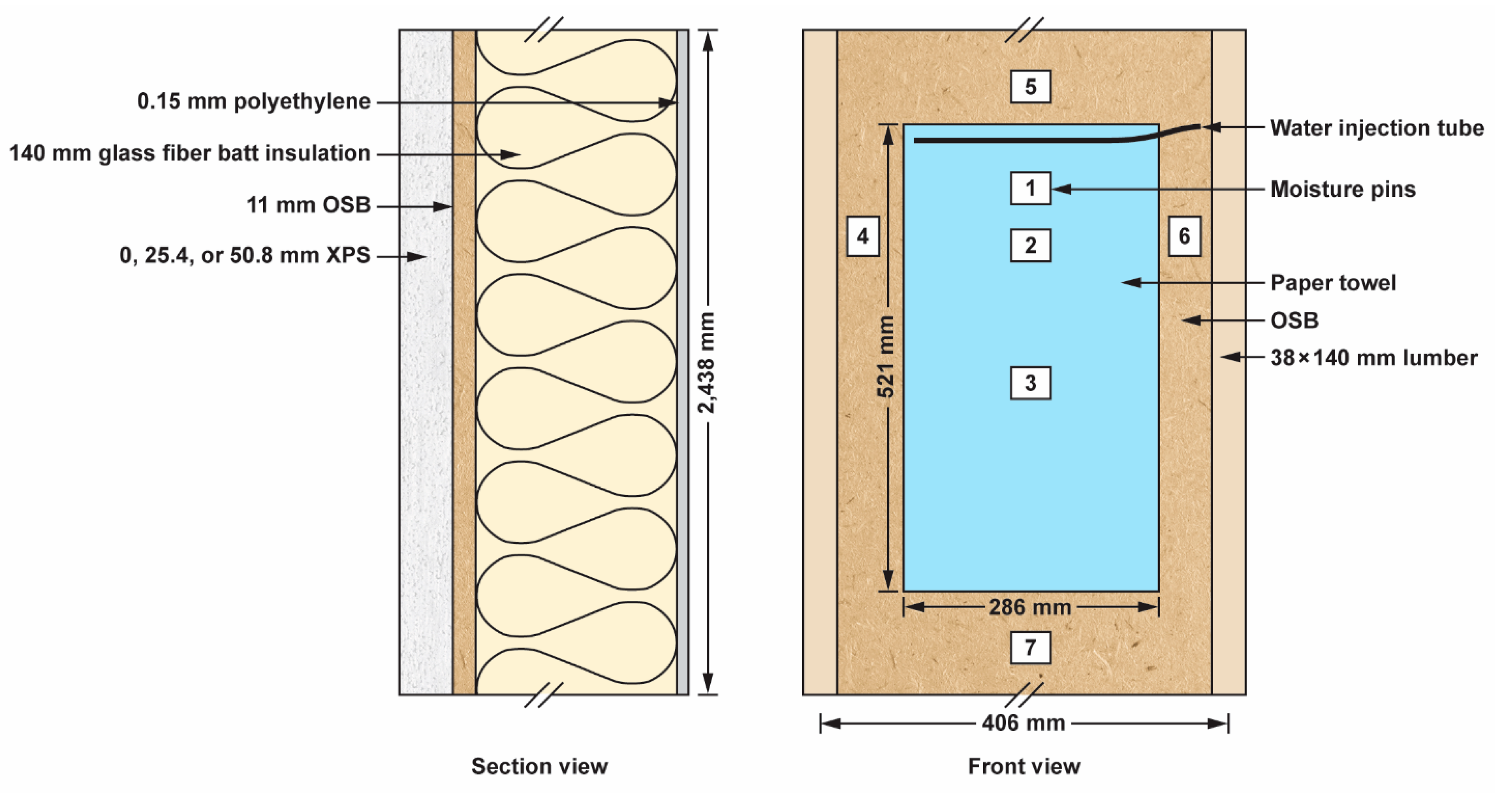
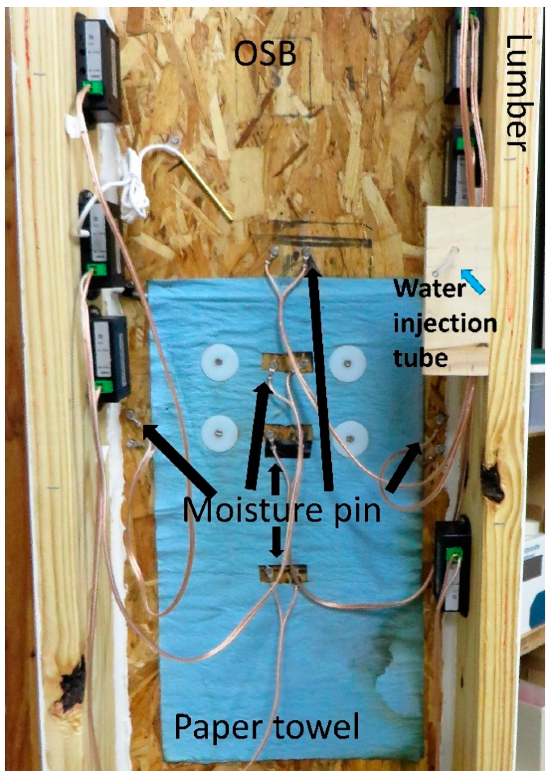
2.1. Wall Assemblies and Wetting System

The test wall assembly was framed with 38 mm × 140 mm (nominally 2″ × 6″) softwood lumber and 11 mm thick (7/16″) OSB sheathing. North American OSB is manufactured to a performance-based standard [24] and the bond classification is Exposure 1. This OSB is typically manufactured with either 100% pMDI binder (polymeric methylene diphenyl diisocyanate) in the face and core layers or phenolic binder in the face plus pMDI in the core. There were only two studs, 2.44 m (8′) tall, spaced 406 mm (16″) apart on center. The same lumber was used to create a short top and bottom plate. Caulking was applied in order to seal lumber joints and the OSB interface after construction. The final open face of the cavity was sealed with 0.15 mm polyethylene sheet taped to the lumber, in order to limit drying to the outward direction, i.e. through the OSB. The polyethylene was penetrated only by a 3.1 mm inner diameter vinyl tube that allowed water to be injected from outside the cavity onto the surface of the OSB, where it was retained by a paper towel [10]. Three small holes in the tube (in center and on each end) allowed a trickle of water to enter the top of the paper towel stapled to the OSB surface. This “wetting system” has been found to yield consistently reproducible wetting of a localized OSB area and promote OSB water absorption. Each injection had a mass of 40 g per day, which wet the paper towel without causing water to run down the OSB sheathing, holding the water against the OSB until it was absorbed or evaporated into the insulated cavity. The paper towel was cut out around the moisture pins, as described below, so that the screws for moisture content measurement went directly into the OSB without touching the paper towel. The rest of the sensors described below were then installed before the cavity was filled with fiberglass insulation to reflect typical wall construction. Finally, the polyethylene vapor barrier was taped to the lumber studs. Figure 1 shows a diagram of the wall construction and location of moisture pins.
This construction was very similar to a traditional wood frame system, allowing direct comparison to field studies. However, unlike in the field, this top plate had an additional lumber layer into which lag screws fixed a steel T with a hole for lifting. A hook fit into this hole, allowing the assembly to be lifted from the ground by the counter-balance mass measurement system described further subsequently.
An overview of wall configurations is provided in Table 1. For some experiments, an additional layer of rigid insulation was added to the exterior of the OSB. This was a 25.4 mm or 50.8 mm thick piece of extruded polystyrene (XPS) attached to the OSB with screws and sealed with caulk near the edges to discourage air infiltration between the OSB and XPS. For the first two experiments, diffusion through the lumber studs was reduced by taping the same 0.15 mm polyethylene plastic (poly) to the outside of the lumber, leaving only the OSB or XPS exposed to laboratory conditions. For other experiments, the framing lumber was either uncovered or painted with a single coat of vapor-retardant paint. For all experiments, the 40 g water injections lasted 4 days for a total of 160 g, with the exception of wall 3, which had a total of 300 g. These last four experiments explore the possible influences of other assembly details and conditions on the moisture redistribution. The injection of 160 g water for most experiments was chosen because this was one of the injections in the field study which motivated this laboratory work and because 160 g provides enough water to see significant effects of redistribution.

2.2. Moisture Content, Temperature, and Relative Humidity Measurements

Moisture pin pairs were used in 5 to 7 locations (Figure 1) to measure electrical resistance, which was calibrated to the moisture content (MC) of the OSB. The “moisture pin pair” did not consist of the traditional driven nails but 18-8 stainless steel sheet metal screws (slotted hex washer head, #6 × 12.7 mm). These were wired to the inputs of a sensor system (Omnisense S-2-2 or S-2-3) which can read the resistance and has inputs for the temperature and relative humidity sensors. The sensors relayed data wirelessly to a base station which was connected to the internet, allowing upload of measured data to an online server.
The primary temperature and relative humidity sensor was an A-1-200 HumiSense temperature and humidity probe (also from Omnisense), while later, an additional RH sensor was added to the cavity as part of the S-2-3, which has a Sensirion sensor built into the system. Both the A-1 HumiSense and S-2-3 built in sensors have uncertainty of ±0.3 °C and ±2% RH. The combination RH/T sensors were mounted on the sides of the studs near the height of the wetting system paper towel.
While the data acquisition system can read and directly present the RH/T readings, the moisture content readings are given as wood moisture equivalent readings. This translation from resistance reading to MC assumes the correlation for Douglas fir, which is not accurate for OSB. Hence, we used a two-step process to calculate the actual MC using correlations described in Boardman et al. [8]. First, we calculated the measured resistance reading (using the Douglas fir correlation to derive it from the reported MC) and then used the OSB MC correlation based on temperature and resistance to calculate a better estimate of the OSB MC. Moisture content is expressed throughout as percentage of dry mass (equivalent to grams of moisture per 100 g of dry material).
While the RH/T readings are assumed consistent throughout the cavity (given the vapor open fiberglass insulation), the MC readings vary based on sensor placement. Three sensors were placed in the field of the paper towel, so they spike upon water injection (Figure 1). One of these sensors (sensor 2 in the middle) was limited to reading the outer ½ of the depth of the OSB by having the screw threads stripped and replaced with insulation near the head of the screw. All other moisture pins measure across the full depth of the OSB and thus pick up the highest moisture content (least resistance) at any depth within the OSB thickness. Two sensors (4 and 5) were placed outside the field of the paper towel, and two more (6 and 7) were later added. These sensors do not spike as much upon water injection but measure the migration of water away from the injection site. Figure 2 shows a photograph of the paper towel with moisture pins installed.
Laboratory conditions were monitored near the wall using a RH/T data logger (Hobo UX100-011) which has uncertainty of ±0.21 °C/2.5% RH. Generally, laboratory conditions were stable, near 24 °C and 45% RH. However, in the summer, the room temperature rose erratically, and the relative humidity sometimes spiked above 55% RH.
To calculate the water vapor pressure given the relative humidity and temperature, the saturation vapor pressure (psat) was calculated using a slightly modified equation from Buck [25], with output in Pa given temperature θ in °C:
p sat ( θ ) = 613.65   exp [ ( 18.729 θ / 227.3 ) θ θ + 257.87 ]
Vapor pressure p was then calculated from p = h·psat, where h is relative humidity (0 ≤ h ≤ 1). To calculate the OSB vapor pressure, a formula from Boardman [9] was used based on a generic OSB sorption isotherm, allowing calculation of the relative humidity h given the moisture content u:
h = 1 exp [ 1520 T ( 1 T 647.1 ) 2.48 ( u 100 ) 17.3 T 0.451 ]
where T is the absolute temperature (K).

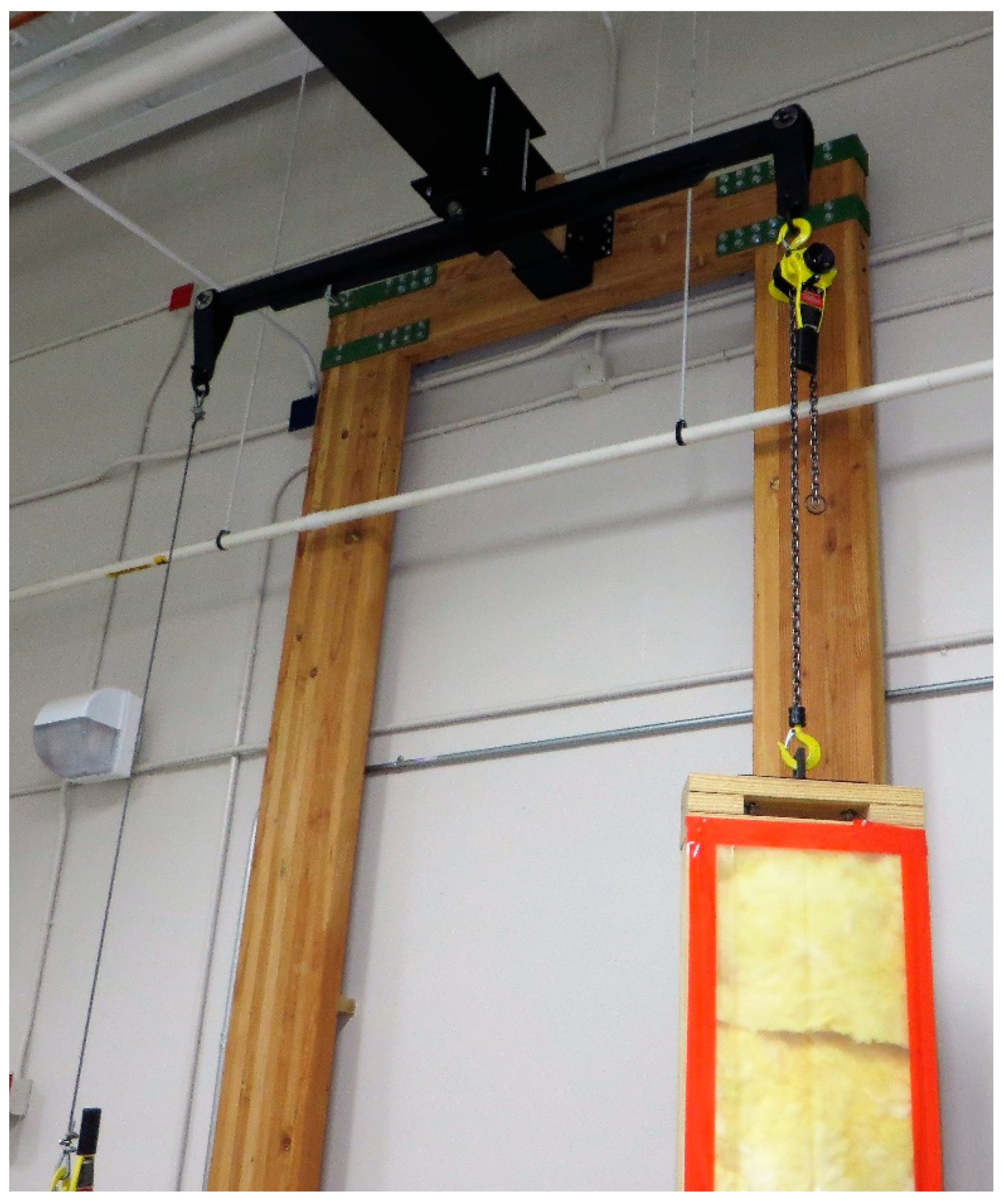
2.3. Load Cell and Counter-Balance System

In order to measure the mass of the wall assembly with accuracy down to the gram, most of the mass of the wall was offset by a concrete block hung in counter-balance using a steel arm held up on a pillow bearing attached to a steel beam that was fixed near the ceiling of the laboratory. On each side of the 1.8 m length steel arm, the wall and concrete block were hung using 680 kg (¾ ton) chain hoists that allow positioning of the loads. Figure 3 shows a photograph of the balance arm attached to a support beam. The concrete block rested above the ground on a metal table, with a wire attached under the block to provide additional mass up to 4 kg when the block was lifted off the table, creating tension in the wire (Figure 4). A 4.5 kg load cell (tecsis XLA) measured this tension between the concrete block and the additional mass, which sat on a lower shelf of the table. The tension in the wire was adjusted by setting small mass calibration cylinders on either the concrete block or the top of the wall to place the load cell in the middle of its range. These mass calibration cylinders were also then used to calibrate the voltage output of the load cell, which was read by another data acquisition system (NI 9237) to yield output in grams. Typical accuracy was ±3 g, with a small drift over time and a noisy signal. The mass measurement system was sensitive to changes in room temperature and affected by changes in room humidity. Corrections for these effects are discussed in Appendix A and Appendix B.

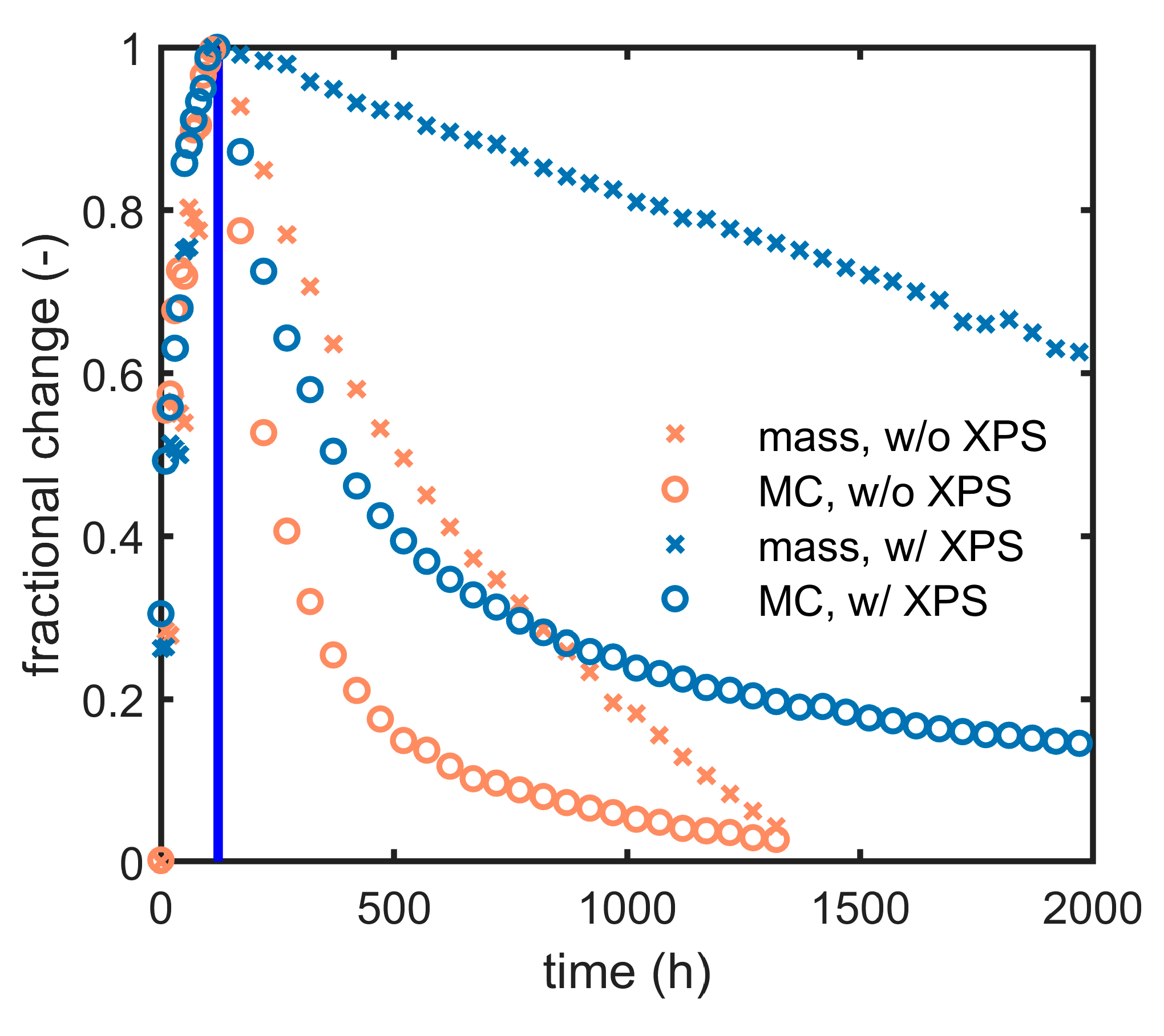
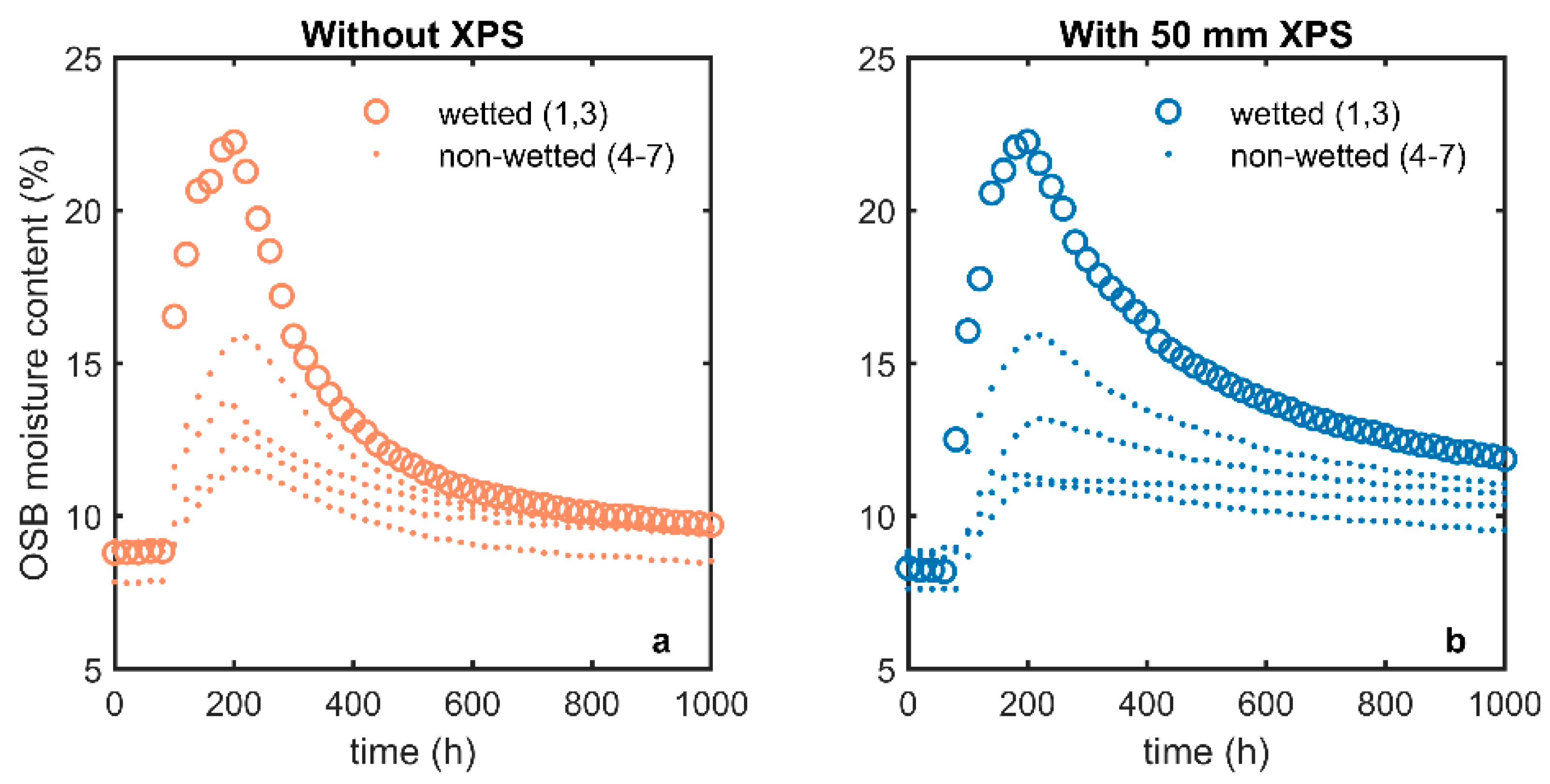
3. Experimental Results

This section reports measurements from the first two experiments, both of which used polyethylene to reduce diffusion through the lumber (see Table 1). The measured fractional change in mass and local moisture content in the wetted area (from the moisture pins) are plotted over time for both experiments in Figure 5. Fractional change, s(t), as a function of time t is defined as
s ( t ) = S ( t ) S init S peak S init
where S(t) is the signal (either mass or moisture content), Sinit is the initial value prior to water injection, and Speak is the maximum value after water injection. The plots start just prior to the water injections. Typically, over 70% of the paper towel area becomes wet after injection, so that pins 1 to 3 inside the field of the paper towel all rise. The MC which represents this wetted area is the average of pins 1 and 3.
Of course, the XPS covered OSB dries much more slowly than exposed OSB alone, but the MC also clearly drops more rapidly than the total mass in both cases. This is the effect hinted at in our earlier field study, which we set out to better understand in this paper. The moisture pin data are plotted in Figure 6 for both experiments. The open circles labeled “wetted” are the average values of two of the pins (1 and 3) in the field of the paper towel and represent the wetted area. Pin 2 is not shown because it reports a lower moisture content, reflecting only the outer half of the OSB. The other four pins are dots labeled “non-wetted”, showing the rise and fall outside the field of the paper towel.
Despite being outside the paper towel, the moisture pins near the towel measure a rise in moisture content, indicating moisture transfer away from the wetted area. Further insight into the moisture transfer mechanisms may be obtained by inspection of the vapor pressures (p) versus time. Figure 7 plots the vapor pressures calculated from RH/T sensors in the laboratory and within the insulated cavity, along with the equivalent values calculated from the OSB MC readings (using the sorption isotherm provided in Equation (2)), both in the wetted region (average of pins 1 and 3) and the non-wetted (nw) region (average of pins 4–7). Vapor pressures were adjusted by a constant offset to match the laboratory value prior to water injection; further details are provided in Appendix C.
In both cases, the cavity vapor pressure is between that of the wetted and non-wetted OSB.
Given these vapor pressure data, a simple diffusion model can provide an estimate of the moisture leaving the system. Such a model, similar to a one-dimensional hygrothermal model, can be validated by the total mass measurement. With such a model in hand, it is then possible to calculate the moisture transfer away from the wetted OSB region. The simple diffusion model is thus used to gain insight into the moisture redistribution, as seen by the moisture pins. An engineering approximation for the moisture redistribution is suggested to capture both the mass loss and moisture content drop. The development of these simple coupled models is described in the following section.

4. Moisture Transfer Model

4.1. Basic Moisture Transfer Mechanisms and Approximations

The simple models developed here approximate the moisture transfer in the wall assembly without accounting for all the complexity of the three-dimensional time-dependent moisture transport that occurs as water moves through the thickness of the OSB under the wetting system, away from the wetting site, into the cavity air, and diffuses through the OSB and lumber studs into the laboratory. The focus was on the drying portion of this moisture transfer, which occurred after several days of injection, because we were seeking to quantify wall drying. During the injection period, the OSB under the paper towel was charged with liquid water while water also evaporated into the cavity air, increasing the relative humidity and hence further distributing the initial water injected. Primary drying occurred at the outer surface of the OSB as water vapor left the assembly. In most experiments, there was also diffusion through the lumber studs. This diffusion was modeled using the standard one-dimensional steady state diffusion mass flow relationship of Fick’s law [26], driven by a vapor pressure difference.
Q = A Δ p R
Here, Q is the rate of water vapor diffusion (g h−1), A is the surface area (m2), R is the resistance to water vapor diffusion (m2 h Pa g−1), and p is water vapor pressure (Pa). The time units are in hours (h) since the process is slow and the data were acquired on an hourly basis. Values of Q were calculated each hour based on the values of p. Each material was represented by a single vapor resistance value; the typical dependence on relative humidity for hygroscopic materials such as lumber and OSB is not included in the model. The model includes additional effective resistance due to the air layers (Rair) on the inside and outside of the OSB. When exterior insulation was added over the outside of the OSB, this further increased the total resistance to moisture flow by Rxps.
This diffusive flow was modeled as three components, one (Qwet) coming from the wetted area of the OSB directly under the paper towel (Awet) and the second (Qnw) from the rest of the area (Anw) of the rectangular piece of OSB. In the majority of the OSB area (Anw), the vapor driving force is the difference between the vapor pressure in the wall cavity (pcav) and the laboratory (plab). The third flow (Qwood) is constituted by diffusion through the lumber studs, driven by the same pressure difference but with different resistance factors, including wood thickness (Rwood) and, in some experiments, a paint layer (Rpnt).
However, validation of Fick’s law was not our objective. This first simple diffusive model was needed in order to account for water leaving the system. However, the moisture pins respond both to the water leaving the system and to moisture redistribution. Our goal was to provide a simple characterization of this moisture redistribution, suitable for use in a one-dimensional hygrothermal model. We did not use a simple linear model, such as in Fick’s law, to model redistribution away from the wetting area. This transfer presumably includes lateral movement inside the OSB, through both diffusion and capillary action and redistribution inside the cavity through the fiberglass insulation. Instead of directly modeling these flows, an empirical near-exponential decay was used to characterize redistribution, with the starting mass value, k, set equal to half the initial water mass measured by the moisture pins. This initial mass depends on the wetted area, fixed at 0.157 m2 to roughly match the rectangular paper towel area. The area of the initially wet OSB is not well defined so the area of the wetted portion was chosen to approximate the paper towel area. Similarly, the moisture content of this area varies by location and is arbitrarily assumed to be represented by the average of moisture pins 1 and 3, which are in the field of the wetted paper towel. The initial water mass used to calculate k also depends on the density of the OSB, which was measured as 540 kg/m3. The assumption of near-exponential decay to describe the mass of injected water subject to moisture redistribution will be explored later by comparing other possible simple models, including pure exponential decay. The near exponential function f(t) is described in more detail by Whitehead et al. [27] and is shown in Equation (5) below, with k as the scale factor (g), c a dimensionless shape parameter, τmrd the time constant (h), and t the time (h).
f ( t ) = k ( 1 1 + c t / τ mrd ) 1 c
Both c and τmrd were used as fit parameters in the moisture balance described below to allow the predicted MC inside the wetted region to track the measured values over time. The c value, which must be above 0, determines this function’s proximity to pure exponential decay.
In addition, because the laboratory conditions were not always constant, it was sometimes necessary to model the moisture sorption in the OSB and lumber studs, as the OSB bulk MC and lumber bulk MC changed to reach equilibrium with the room. A simplified method of calculating the moisture transfer from sorption was used by TenWolde [28] and Boardman and Glass [29] to model whole building moisture transfer. The model assumes that the material effectively equilibrates with the average relative humidity over its recent past. Here, it is based on the vapor pressure (plab), but the same exponentially weighted average was used:
p ave = j = 1 400 p lab ( j ) · w ( j , τ sorp ) j = 1 400 w ( j , τ sorp )
where τsorp is a time constant for sorption (set to 100 h) and w is a function that applies exponential weighting over the previous 400 h:
w ( j , τ sorp ) = e 0.5 j / τ sorp
so that the rate of moisture transfer from sorption each hour is represented by:
Q sorp = A ( p lab p ave ) R air + R sorp
Here, Rsorp represents the resistance to diffusion in combination with sorption and is another fitting parameter in the moisture balance described in the next section. The full model uses two Qsorp terms, one for the OSB and the other for the lumber, which have different resistance terms related to paint on the lumber or exterior insulation sometimes covering the OSB, as well as different areas. The time values used for averaging and the sorption time constant are discussed in Appendix B.

4.2. Moisture Transfer Model for the Whole Wall and for the Water Injection Site

The predicted mass of injected water remaining in the wall assembly, m, can be compared to the total measured mass at each hour. The predicted total mass at time ti was based on the mass at the previous hour (ti−1) and the moisture flows Q from diffusion and sorption (Equation (8)) for a time step Δt set to 1 h:
m ( t i ) = m ( t i 1 ) + Δ t ( Q wet Q nw Q wood + Q sorp )
Q wet = A wet ( p wet p lab ) R air + R osb
Q nw = A nw ( p cav p lab ) 2 R air + R osb
Q wood = A wood ( p cav p lab ) 2 R air + R wood + R pnt
Similarly, the predicted moisture content for the wetted area, u, can be compared to the measured moisture content at each hour. This again was based on the previous hour and the moisture flows from outward diffusion (Qwet), inward diffusion into the insulated cavity (Qin), redistribution (Qmrd) within the OSB or the cavity away from the injection site, and sorption (Qsorp) scaled by the ratio of wetted area to total area (Awet/Aosb):
u ( t i ) = u ( t i 1 ) + Δ t ( Q wet Q in Q mrd + Q sorp A wet A osb ) 10 ρ d , osb A wet L osb
where ρd,osb is the dry density of OSB (540 kg m−3) and Losb is its thickness (11 mm).
Q in = A wet ( p wet p cav ) R air + R osb / 2
Q mrd = f ( t i 1 ) f ( t i ) Δ t
The moisture redistribution (Qmrd) is strongly dependent on Equation (5) modeling the mass of water moving out of the wetted area into the surrounding OSB, as well as further net transfer due to redistribution in the air. In those cases where external insulation was added to the OSB, the additional term Rxps was added to Equations (8), (10), and (11).
This model was implemented in a spreadsheet with hourly time steps. The drying simulation began after the final injection, when the MC readings in the OSB reached their maximum; this time was assigned t = 0. The initial moisture content, u(t0), was set to the peak MC measured by the moisture pins. However, the initial value of total mass, m(t0), was allowed to vary somewhat from initial measured mass. When the peak MC was reached and the simulation started, the mass flow was still far from steady state, so there was little chance of matching the predicted and measured m. It took an additional day or two for the mass flows to stabilize, so the starting value, m(t0), was adjusted to minimize the difference between predicted and measured values after the system was closer to steady state. Furthermore, it was not possible to use the mass corresponding to the MC reading because an unknown amount of injected water had already moved outside the wetted area before the model even began, given that the injections happened over multiple days.

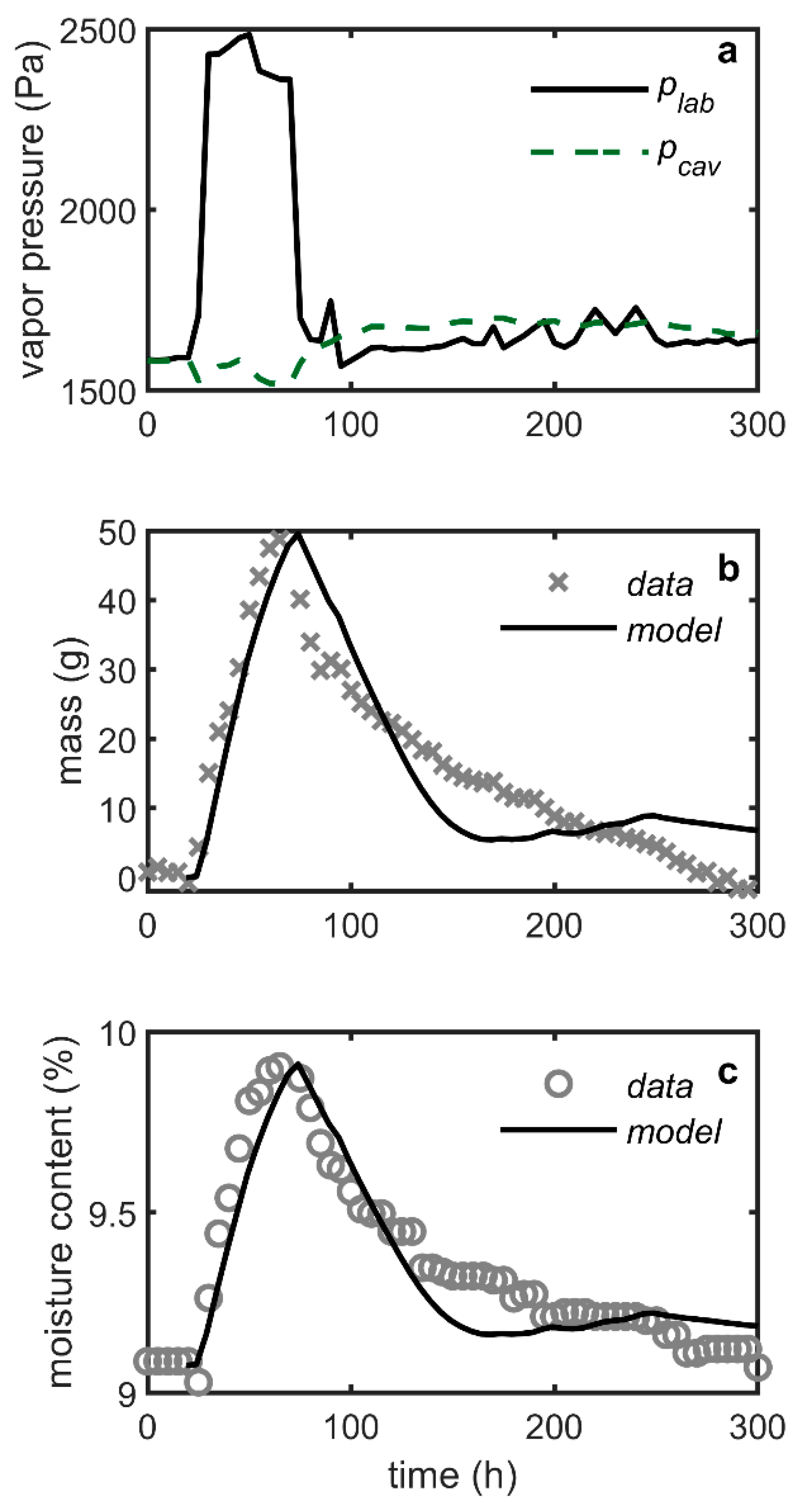
5. Modeling Results and Discussion

To obtain vapor resistance values for OSB and XPS, the two initial experiments previously discussed were performed with plastic covering the studs, leaving only the OSB or XPS exposed. Modeling results are discussed in the first section and R values obtained were starting points for modeling of subsequent experiments. The R value for OSB corresponds to literature values, as expected. Next, four experiments were performed, with variations in water injection mass, presence of XPS insulation over the OSB, stability of laboratory RH conditions, and paint on the outside of the exposed lumber studs (see Table 1). The second section presents overall optimized resistance values for lumber and XPS based on these (non-poly) experiments, demonstrating the success of the simple model under more “field-like” conditions. The success of the diffusion model which tracks the total mass was not surprising, but the ability to track the local OSB moisture content demonstrates the usefulness of the engineering approximation for the moisture redistribution. In the third section, the near-exponential form of Equation (5) is further motivated by examining model fits when other functional forms are assumed. The early rapid transfer away from the injection site captured in the near-exponential form is seen to be important for modeling the measured MC data.

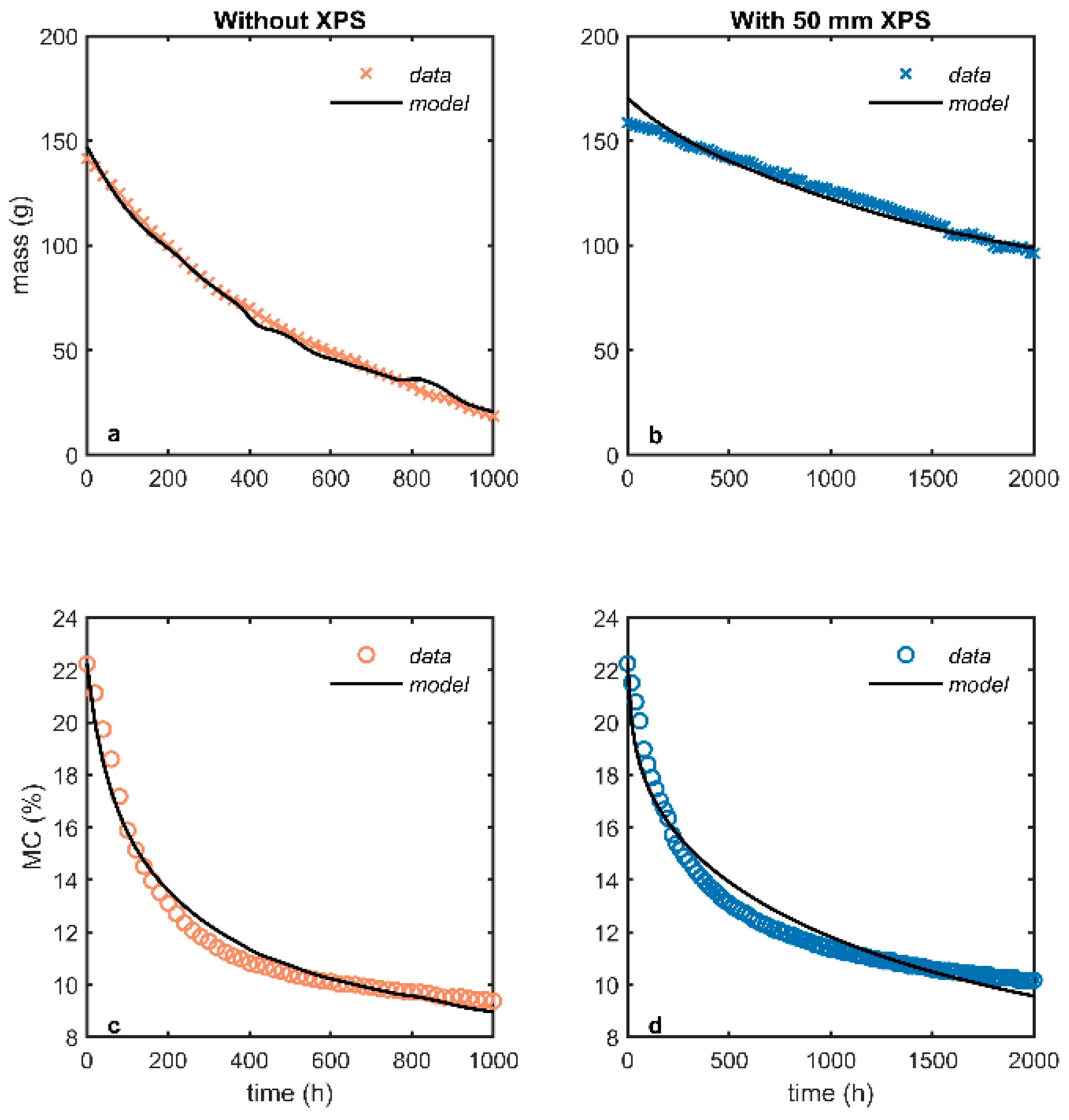
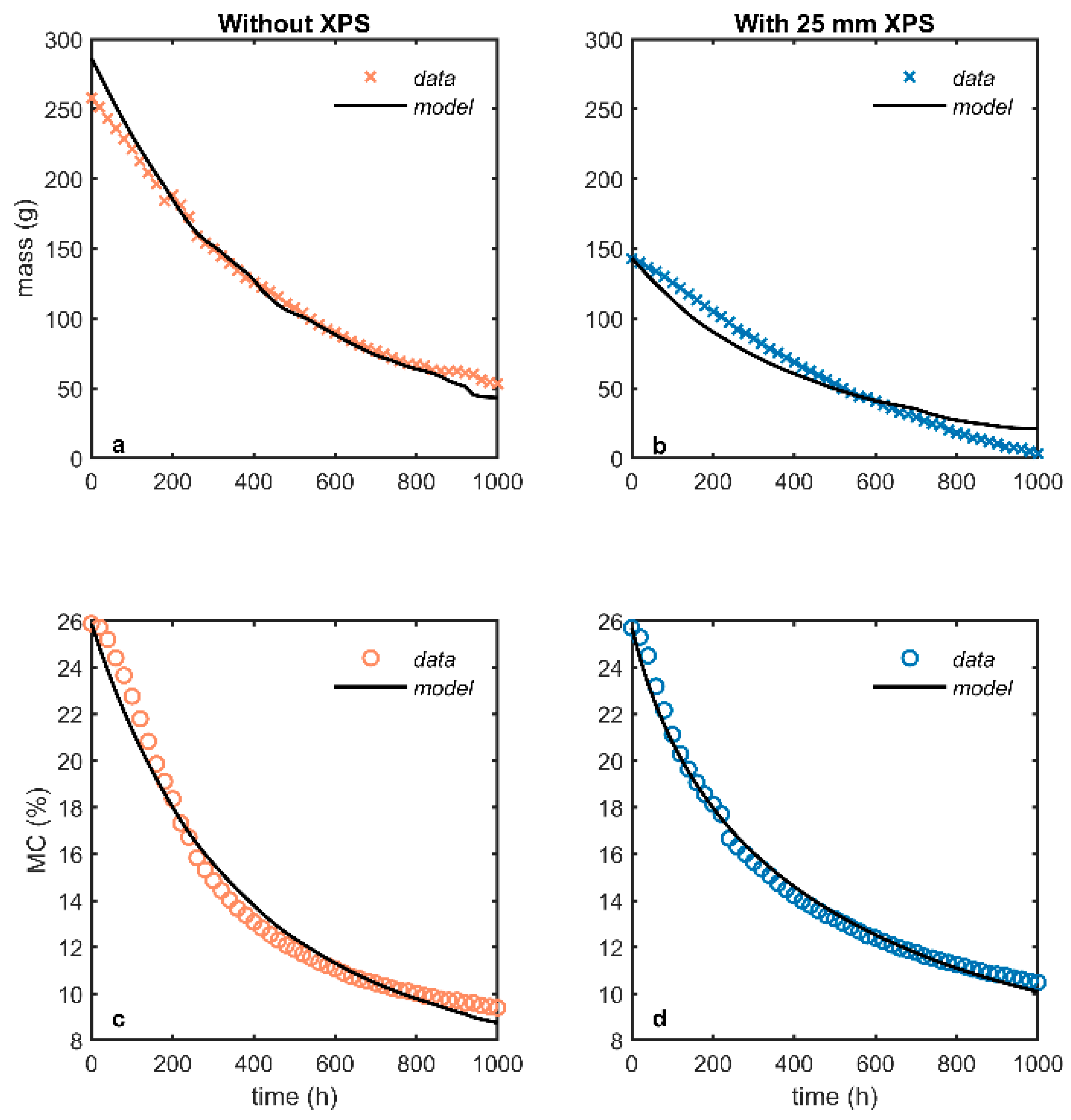
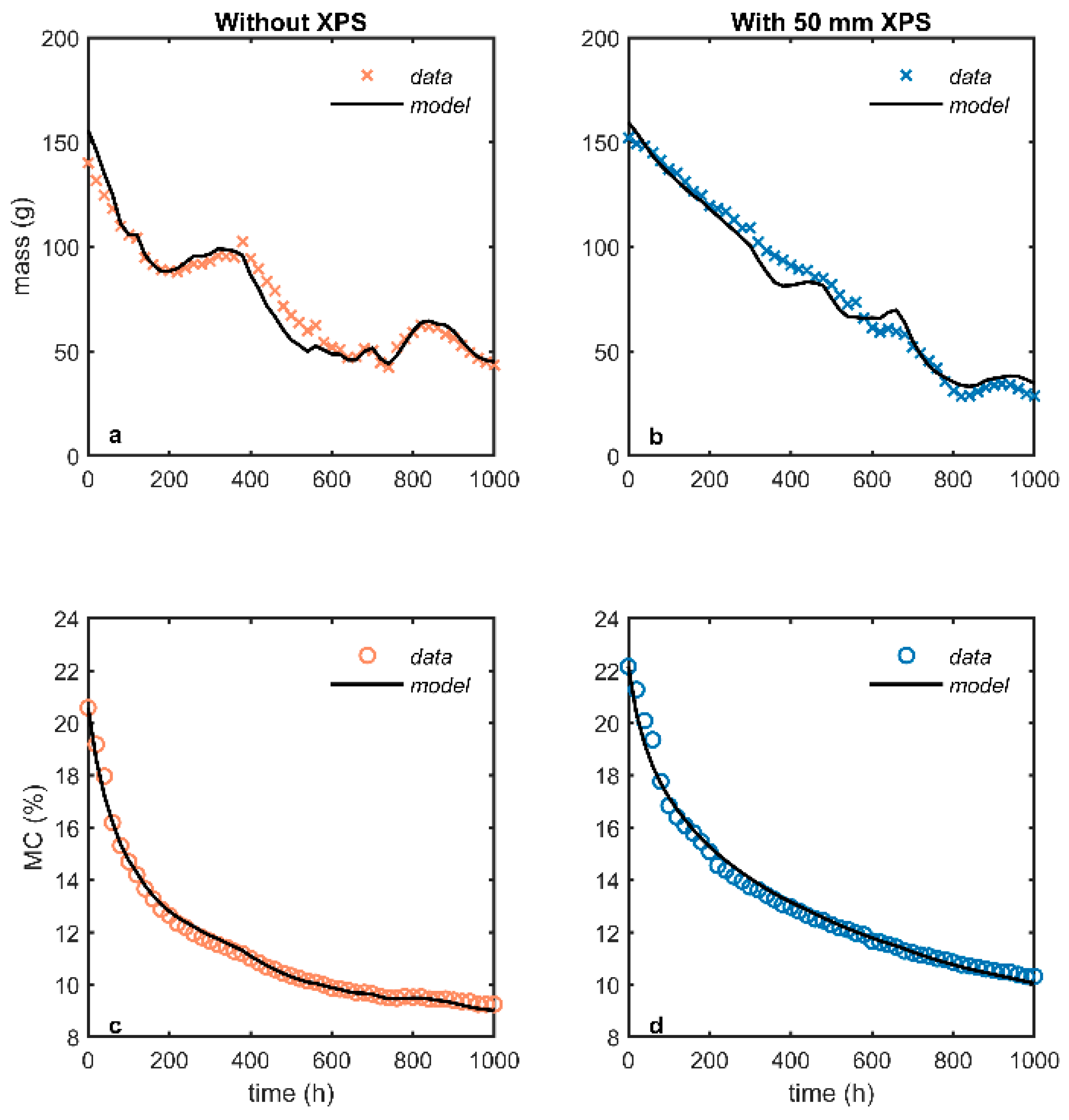
5.1. Modeling versus Measured Drying Curves

5.1.1. Results for Poly Walls

In the first experiment, the wall with only the OSB exposed was injected with 160 g of water over four days and subsequent drying was monitored using the balance and moisture pins. The model was optimized by adjusting Rosb, with diffusion through the framing assumed to be negligible due to the polyethylene covering, in order to minimize the difference between measurement and model prediction for both the MC within the wetted area and the total mass of injected water remaining in the wall. Model predictions are compared with measurement on the left side of Figure 8. The resulting OSB vapor resistance was equivalent to a vapor permeability of 1.2 ng Pa−1 s−1 m−1, which corresponds to a diffusion resistance factor of 170. Recall that the water vapor diffusion resistance factor is the ratio of the vapor permeability of still air to that of the material and is thus dimensionless. We assumed that the permeability of air was 198 ng Pa−1 s−1 m−1 based on the calculation methods in ASTM standard E96 [30], using a temperature of 23 °C and pressure of 1 bar. This value for OSB is between the 40% and 70% RH levels for OSB reported in the literature [31,32,33,34].
In the second, long running experiment, 50.8 mm of XPS was added to cover the OSB and, again, 160 g of water was injected. The model assumed the OSB resistance value just reported and was optimized to find the resistance of XPS. Model predictions are compared with measurement in the right half of Figure 8. The resulting XPS permeability was 2.5 ng Pa−1 s−1 m−1, which corresponds to a diffusion resistance factor of 79. This value for XPS is lower than the range of values (94 to 208) reported in the literature [31,32,35]. Furthermore, this value was still too high to model the non-poly wall results discussed next, which used an XPS resistance factor of 55. In all cases, the XPS was caulked to the OSB surface, but in the case of the poly wall, the XPS was also taped to the polyethylene which covered the lumber. We suggest that these lower XPS vapor diffusion resistance factors are realistic for field work, where water vapor can diffuse through alternative paths in addition to directly through the XPS or possibly be carried away by air leakage between the XPS and OSB.

5.1.2. Results for Non-Poly Walls

The next four experiments included diffusion through the lumber studs since they were not covered with plastic, with and without a paint layer on the exposed lumber studs. The paint was added to reduce the diffusion through the studs but had no significant effect. These and other variations are detailed in Table 1.
Optimizing the model across all four datasets, which share Rosb, Rxps, Rair, Rsorp, and Rpnt, yielded a wood permeability of 3 ng Pa−1 s−1 m−1. This corresponds to a diffusion resistance factor of 63. This value for wood is between the 50% and 75% RH levels for soft woods like spruce, pine, or fir reported in the literature [32,36,37], again showing good agreement with literature values. Table 2 summarizes all the optimized R values in units native to the model (Pa h m2 g−1). Regarding moisture redistribution away from the injection site, the average values of c and τmrd for the near-exponential decay model of the lateral movement were 1.44 and 168 h, respectively. Table 3 summarizes the c and τmrd values for each wall, beginning the exploration of the parameter variability depending on insulation levels and water injection amounts.
These resistance values and moisture redistribution parameters allow good agreement between the predicted MC inside the wetted area and that measured by the moisture pins, as well as the expected agreement between the total mass of added water left in the system measured by the balance and that predicted by the model. Figure 9 plots the predicted versus measured values for the first two experiments (wood), while Figure 10 shows the same plots for the last two (paint).

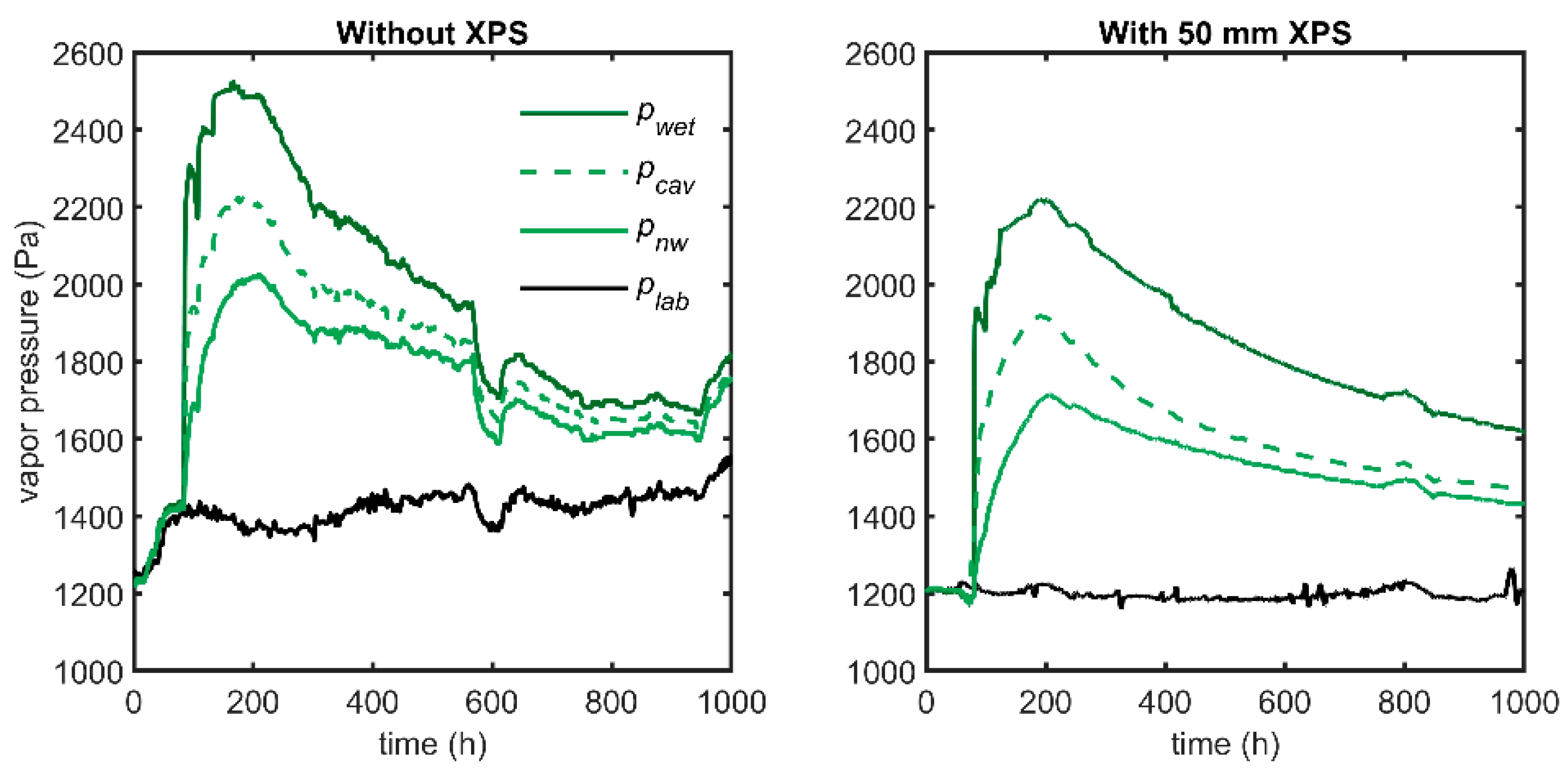
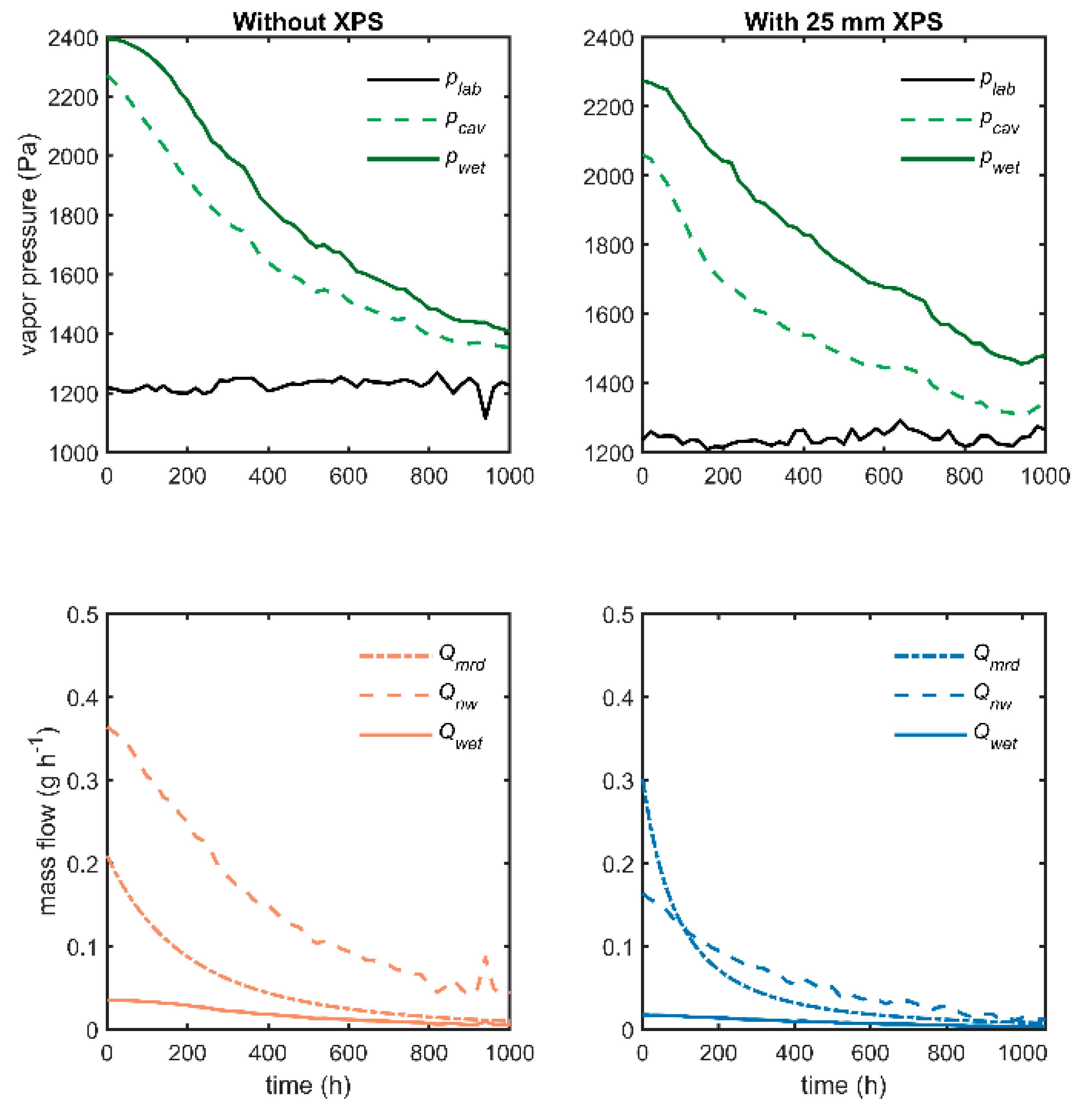
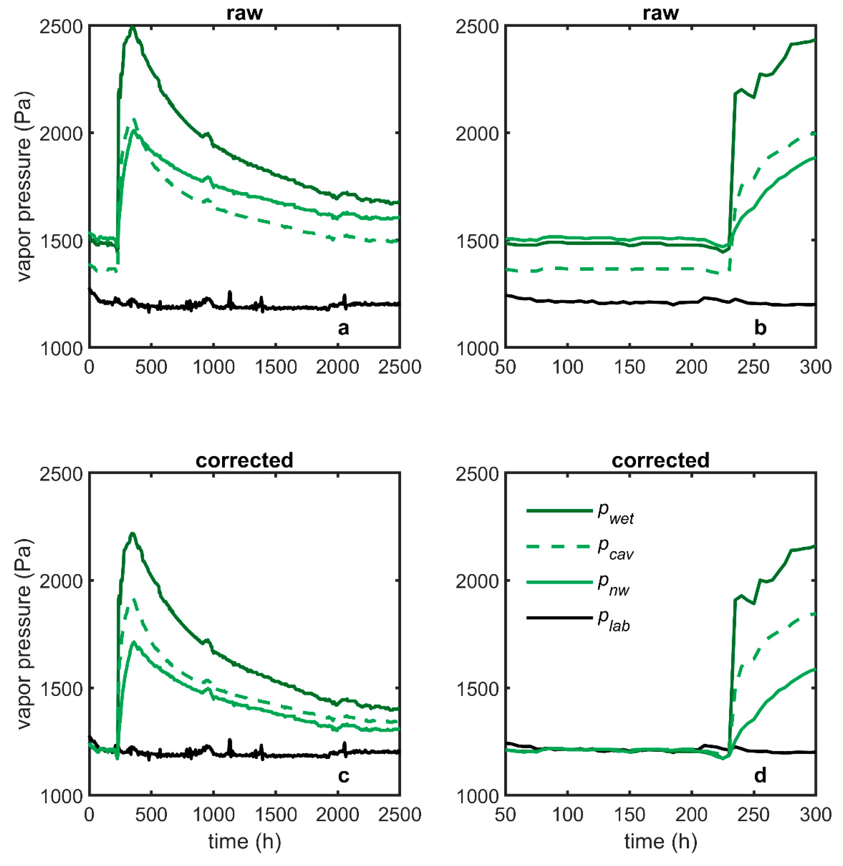
5.2. Water Vapor Pressure and Component Moisture Flows

The driving vapor pressure, p, and resulting moisture flows, Q, are plotted for the same four experiments in Figure 11 and Figure 12. As expected, the vapor pressure in the OSB wetted region is always above that in the cavity, driving moisture into the cavity air and into the ambient laboratory air. The moisture flow from the wetted area itself (Qwet) is smaller than the flow from the rest of the OSB (Qnw) because the area is much smaller. More interesting is that the movement of moisture away from the wetting site (Qmrd) is much higher than flow due to diffusion (Qnw) very early in the drying, as moisture moves laterally in the OSB and into the cavity air. The magnitude of these flows equalizes as the drying continues. The ability to calculate Qmrd is the primary fruit of this modeling effort.

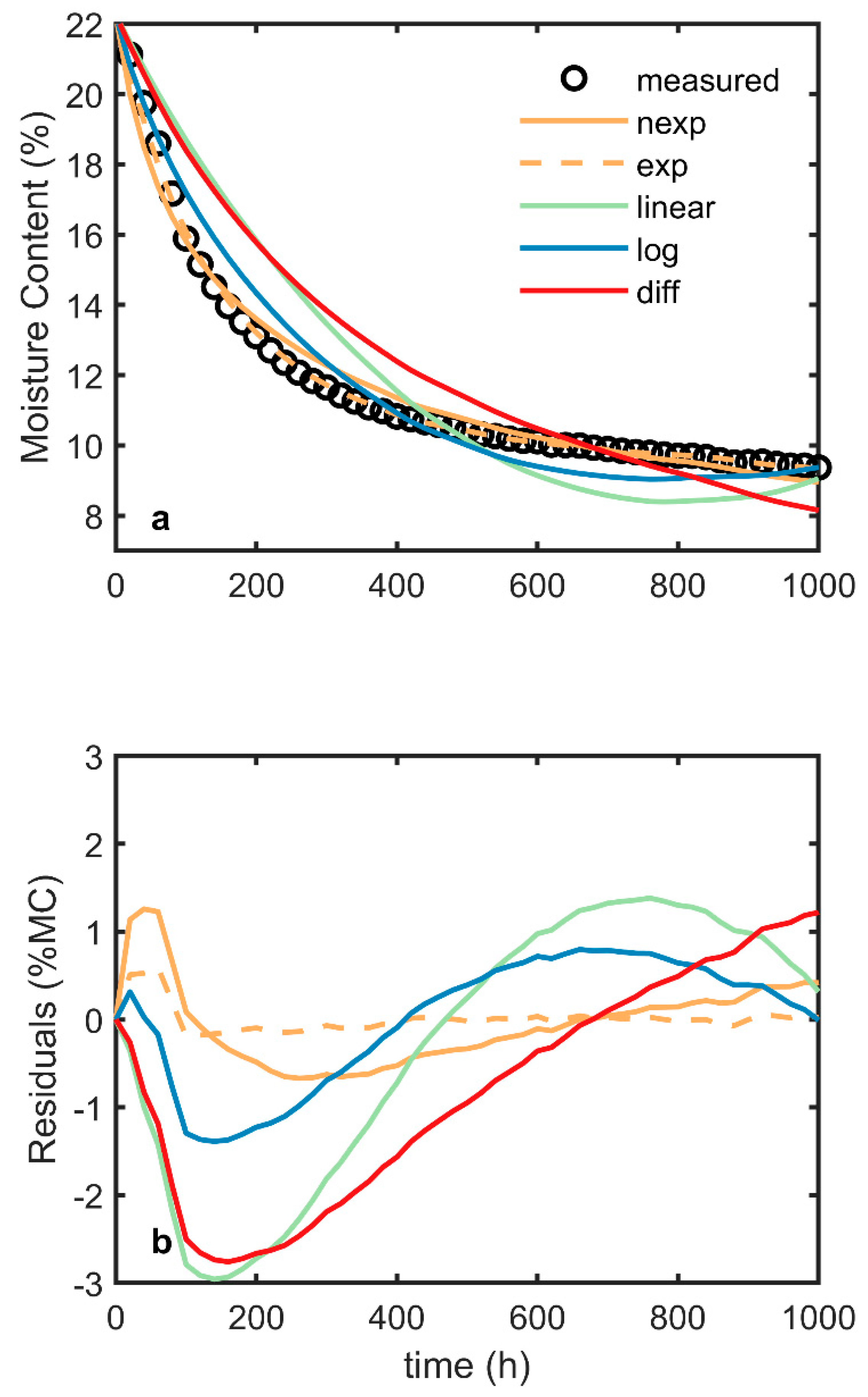
5.3. The Shape of the Redistribution Function

No attempt has been made to physically model the complex physics which control the moisture transfer away from the injection site. Equation (5) has a useful form and fits the data well. To see how well it fits, this near-exponential form, labeled “nexp” on the following graphs, is compared with four simple alternatives. The root-mean-square-error (RMSE) between model MC and measured MC from the moisture pins is reported to quantify the fit results. Results for most models and all runs are presented in Table 4. The first model, labeled “diff”, attempts to use the vapor pressure difference and some lateral resistance to track the moisture flow. The difference was that between pwet in the wetted area and pnw representing the OSB outside of the wetted area. The effective resistance was allowed to vary in order to obtain the best fit. The results in Table 4 show that this is the worst of the models, primarily because it does not have enough driving force, although the shape of the curve is good. This suggests that additional physical mechanisms are at work in moisture redistribution beyond diffusion laterally through the OSB—for example, capillary transport and evaporation. The rest of the models use different simple functional forms to fit the data, each using two fit parameters, a and b, in the first two cases. The equations explored are a linear fit (Qmrd = at + b), a logarithmic fit (labeled “log”, Qmrd = a·ln(t) + b), and a pure exponential fit (labeled “exp”) which uses the difference in mass between adjacent hour entries like the near-exponential function to calculate Qmrd. Figure 13 plots measured MC and the predictions from all the forms for the poly, w/o XPS wall (top), along with the residuals (bottom).
The near-exponential form of Equation (5) does well but is sometimes beaten by the pure exponential. Both illustrate the importance of the high Qmrd early in the drying and the rapid reduction of this contribution to moisture movement.
One practical drawback of using the pure exponential form when analyzing field data is the lack of a consistent initial value. Across all six experiments, the pure exponential model initial value varied from 44% to 31% of the initial mass in the wetted area. Without full mass data to help tune the models, it is difficult to guess the correct starting mass in the wetted area, and a good fit is dependent on this value. The near-exponential form avoids this problem, making it more practical for the evaluation of field data and use in one-dimensional hygrothermal models, since the value of k was fixed as half of the water mass in the wetted area, as measured by the MC at the start of the model. The c and τmrd parameters allow a good fit but are not as sensitive to obtaining exactly the correct value. Table 5 illustrates this by showing the RMSE when the redistribution function can vary only one fit parameter, τmrd. In this case, k is fixed as half of the water mass in the wetted area for both the pure and near-exponential models, and c = 1.44, the average across the non-poly walls when using the near-exponential model. In all but one case, the near-exponential function has a lower RMSE.

5.4. Further Discussion

This model makes it clear that moisture redistribution away from the injection site but not leaving the system is rapid at first but quickly drops below that from diffusion out of the system. Related to this result is the observation that pcav is only slightly less than pwet and that pcav is the primary driver of moisture loss from the system. We speculate that water is rapidly distributed within the cavity by multiple mechanisms which include lateral diffusion within the OSB, capillary transport, and evaporation from the injection site into the cavity air. As a result of this moisture redistribution, the MC read by the moisture pins in the field of the paper towel drops rapidly at first, but this does not correspond to rapid moisture loss from the system. This moisture redistribution reduces the risk of local moisture damage at the injection site but does not correspond to what we usually mean by drying—that is, moisture exiting the wall assembly.
As previously mentioned, we intend for the approximation of the moisture redistribution, which is captured in the model by both Qmrd and Qin, to be helpful when creating one-dimensional hygrothermal models of drying after water injection. The work of Boardman, Glass, et al. [23] started exploration of this modeling using field data and assumed a near-exponential shape for the moisture sink. In the case of the “wood w/ XPS” laboratory data measured in this work, the relevant moisture sink to try in capturing field conditions would be a near-exponential approximation with k = 80 (half of the injection), c = 1.17 and τ = 271 h, based on the sum of Qmrd and Qin. This is close to the Qmrd values c = 1.14 and τ = 168 h because Qin is small, similar to the Qwet values, which are much smaller than Qmrd soon after the injection. This earlier work used a larger k value (85% to 55% of injection), with default c = 0.79 and τ = 75 h applied to all tested cases. This default produced adequate results, tracking the MC of the wetted area as it decayed, with a RMSE of 2.6% MC. The present manuscript will inform ongoing work to improve the one-dimensional hygrothermal modeling of the field data.

6. Conclusions

We collected data on a typical full-size North American wood-frame exterior wall assembly, aiming to better understand the moisture flows from a wetted area of OSB. A mass measurement system tracked moisture leaving the assembly, while moisture pins tracked localized OSB moisture content. The wetted OSB area dried faster than the whole assembly, indicating moisture redistribution within the assembly. A simple model was developed to characterize this moisture redistribution for use in one-dimensional hygrothermal models.
The simple engineering model mimics one-dimensional hygrothermal models by calculating moisture loss from the system driven by vapor pressure differences between the insulated cavity and the exterior of the assembly. The vapor pressure was measured using relative humidity and temperature sensors in the cavity. The model also uses a near-exponential decay function to characterize moisture redistribution. Together, these two models can track the moisture flows from the wetted OSB area, partitioning the flow between moisture leaving the assembly (as would typically be calculated by a one-dimensional hygrothermal model) and redistribution within the assembly (which is handled in a one-dimensional model using a moisture source or sink, since redistribution is an inherently multi-dimensional process). In this initial characterization of the redistribution function, parameter values were provided that were suitable for room temperature conditions with and without XPS insulation covering the OSB. Further work will be undertaken to refine the redistribution function when it is applied to the field data which inspired this laboratory study.

Author Contributions

Conceptualization, C.R.B. and S.V.G.; methodology, C.R.B., S.V.G., and S.L.Z.; software, C.R.B.; validation, C.R.B. and S.V.G.; formal analysis, C.R.B.; investigation, C.R.B.; writing—original draft preparation, C.R.B.; writing—review and editing, C.R.B. and S.V.G.; visualization, S.V.G. and S.L.Z.; supervision, S.L.Z. All authors have read and agreed to the published version of the manuscript.

Funding

This research received no external funding.

Acknowledgments

This work was funded by the USDA Forest Service, Forest Products Laboratory. The authors gratefully acknowledge the help of many FPL colleagues during the course of this investigation. Randy Wruck was especially helpful in the design and realization of the mass-balance measurement system. This manuscript was improved by comments from Marshall Begel and Carl Houtman.

Conflicts of Interest

The authors declare no conflict of interest.

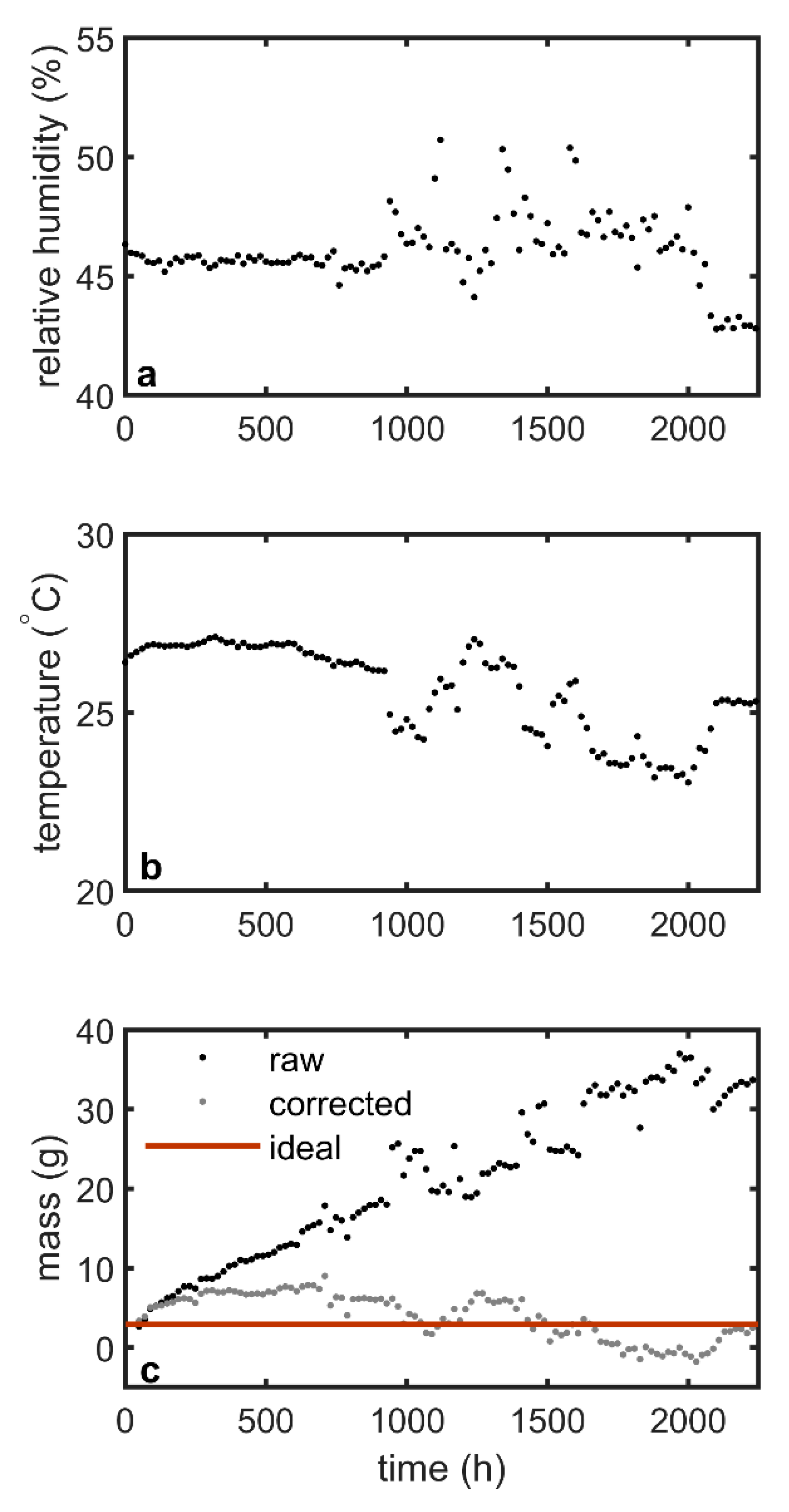
Appendix A. Load Cell Drift and Temperature Correction

A metal counterweight was placed on the wall mass balance to evaluate the effects of drift and temperature change on the load cell which provides the mass measurement. The mass reading from the load cell in an ideal system would have been constant. The room conditions were maintained near 46% RH and 25 °C, with small fluctuations, as shown in Figure A1a,b.
Mass readings showed both load cell drift and the effects of temperature changes. Over the three-month test period, the mass drifted by nearly 40 g, as shown in Figure A1c. The first 50 h of the data were excluded since load cells typically do not stabilize immediately after having a stress placed on them. During the time period from 200 to 600 h, when the temperature was nearly constant, the drift was 14.5 mg/h. After 930 h, the temperature became more variable, which affected the mass output such that a reduction in temperature produced an increase in mass reading. Evaluation of five regions with significant temperature changes resulted in an average temperature effect of −4.2 ± 0.4 g/K.
These estimates of the drift and temperature effects were used as starting points to develop a correction function which could be applied to each hourly mass reading. This function applied a constant drift correction for each hour that had passed and a temperature correction based on cumulative hourly temperature changes. The resulting corrected mass reading is shown in Figure A1c, along with the raw and ideal output. The optimized drift value used was 11.8 mg/h and temperature correction was −4.1 g/K. This correction was applied to all mass readings.
Figure A1. Laboratory conditions (a,b) during constant mass experiment, with raw mass and corrected mass (c).
Buildings 10 00141 g0a1

Appendix B. Calibration of Simple Sorption Model

During some of the experiments, the RH in the laboratory was not well controlled, so the mass reading of the wall was affected by not only the mass leaving the system after the water injection but also mass gain or loss as the exposed lumber studs and OSB moved toward a new equilibrium with the changed room RH. We used a simple approximation for mass transfer due to this sorption effect, based on the RH history of the room, as outlined in Equations (6)–(8). In order to help improve this approximation, we conducted a brief experiment in which the wall had no water injection but experienced a significant spike in room RH. The wood studs were enclosed in plastic, but the full OSB surface was exposed to the room, so the mass of the system changed due to the initial increase and then decrease in room RH. During this time, the room temperature was near 26 °C. The mass and temperature corrections discussed in Appendix A were applied to the mass readings from the load cell. Figure A2 plots the room vapor pressure (a) and associated mass change (b).
Figure A2. Laboratory conditions (a) and associated mass response (b) and MC response (c) during RH spike, showing sorption model fit.
Buildings 10 00141 g0a2
A fit to this mass data was optimized with the sorption time constant, τsorp, set to 100 h. The representative OSB vapor resistance for sorption was 560 Pa h m2 g−1. Assuming the same OSB permeability used in the full model, this resistance represents 21% of the OSB depth. Figure A2 plots the total mass, measured by load cell, with the model prediction (b) and the measured MC with the predicted MC (c). These predictions were produced using the model described in Equations (9)–(15) but neglecting all the moisture transfer terms except Qsorp for the OSB (the framing lumber was covered).

Appendix C. Vapor Pressure Coordination with Room Vapor Pressure

In all the graphs and calculations for this work and the associated models, we used corrected vapor pressures. The baseline was always the laboratory vapor pressure, calculated directly from the RH/T sensor. The cavity and OSB vapor pressure readings were adjusted with a simple additive offset to match the laboratory just before the water injection started. This correction essentially “tared” the vapor pressures so that differences in vapor pressure as a result of water injection could be used for modeling. The experimental uncertainty in vapor pressures at different locations in the wall assembly would otherwise make the uncorrected values useless. The measured data supported the assumption that the wall assembly had effectively reached equilibrium with the laboratory conditions prior to water injection.
Figure A3 shows the raw (uncorrected) values of vapor pressure for the poly w/ XPS case (a), along with a close-up of the pressure before injection (b).
Figure A3. Vapor pressure before and after water injection: raw (uncorrected) values (a,b) and corrected values (c,d).
Buildings 10 00141 g0a3
The baseline was assumed to be from 80 to 110 h, for which the average vapor pressures were plab = 1214 Pa, pcav = 1367 Pa, pwet =1487 Pa, and pnw = 1511 Pa. The three latter values were lowered by constants of 153, 273, and 297 Pa to produce the corrected values used in subsequent analysis. A close-up of the corrected data is plotted in Figure A3d, along with the full data (c).
The offsets for other datasets had a similar pattern. All the offset corrections for the insulated cavity, wetted OSB, and non-wetted OSB are presented in Table A1.
Table A1. Vapor pressure corrections to match laboratory.
NumberLabelVapor Pressure Correction (Pa)
--pcavpwetpnw
1Poly, w/o XPS201340327
2Poly, w/ XPS153273297
3Wood, w/o XPS145327216
4Wood, w/ XPS253430346
5Paint, w/o XPS203398403
6Paint, w/ XPS144311278

References

  1. Tenwolde, A.; Rose, W.B. Moisture control strategies for the building envelope. J. Therm. Insul. Build. Envel. 1996, 19, 206–214. [Google Scholar] [CrossRef]
  2. Lstiburek, J. Understanding vapor barriers. ASHRAE J. 2004, 46, 40–50. [Google Scholar]
  3. Saber, H.H.; Maref, W. Field research study for investigating wetting and drying characteristics in wood-framing walls subjected to cold climate. J. Build. Phys. 2019, 174425911989118. [Google Scholar] [CrossRef]
  4. Van Belleghem, M.; Steeman, M.; Janssens, A.; De Paepe, M. Heat, air and moisture transport modelling in ventilated cavity walls. J. Build. Phys. 2014, 38, 317–349. [Google Scholar] [CrossRef] [Green Version]
  5. Tariku, F.; Simpson, Y.; Iffa, E. Experimental investigation of the wetting and drying potentials of wood frame walls subjected to vapor diffusion and wind-driven rain loads. Build. Environ. 2015, 92, 368–379. [Google Scholar] [CrossRef]
  6. Lstiburek, J.W.; Mitchell, J. Water & walls. ASHRAE J. 2013, 55, 72–80. [Google Scholar]
  7. Lstiburek, J.W. Double, double toil and trouble: Macbeth does vapor barriers. ASHRAE J. 2013, 55, 56–62. [Google Scholar]
  8. Boardman, C.R.; Glass, S.V.; Lebow, P.K. Simple and accurate temperature correction for moisture pin calibrations in oriented strand board. Build. Environ. 2017, 112, 250–260. [Google Scholar] [CrossRef] [Green Version]
  9. Boardman, C.R.; Glass, S.V.; Munson, R.; Yeh, B.; Chow, K. Field Moisture Performance of Wood-Framed Walls with Exterior Insulation in a Cold Climate; U.S. Department of Agriculture, Forest Service, Forest Products Laboratory: Madison, WI, USA, 2019; pp. 1–42.
  10. Van Straaten, R. Measurement of Ventilation and Drying of Vinyl Siding and Brick Clad Wall Assemblies. Master’s Thesis, University of Waterloo, Department of Civil Engineering, Waterloo, ON, Canada, 2004. [Google Scholar]
  11. Smegal, J.; Lstiburek, J.; Straube, J.; Grin, A. Moisture-related durability of walls with exterior insulation in the Pacific Northwest. In Proceedings of the Thermal Performance of the Exterior Envelopes of Whole Buildings XII International Conference, Clearwater Beach, FL, USA, 1–5 December 2013. [Google Scholar]
  12. Ojanen, T. Improving the drying efficiency of timber frame walls in cold climates by using exterior insulation. In Proceedings of the Thermal Performance of the Exterior Envelopes of Buildings VII International Conference, Clearwater Beach, FL, USA, 6–10 December 1998. [Google Scholar]
  13. Hazleden, D.G.; Morris, P.I. The influence of design on drying of wood-frame walls under controlled conditions. In Proceedings of the Performance of Exterior Envelopes of Whole Buildings VIII International Conference, Clearwater Beach, FL, USA, 2–7 December 2001. [Google Scholar]
  14. Schumacher, C.J.; Shi, X.; Davidovich, D.; Burnett, E.F.; Straube, J.F. Ventilation drying in wall systems. In Proceedings of the Second International Conference on Building Physics, Leuven, Belgium, 14–18 September 2003. [Google Scholar]
  15. Teasdale-St-Hilaire, A.; Derome, D.; Fazio, A. Behavior of wall assemblies with different wood sheathings wetted by simulated rain penetration. In Proceedings of the Performance of Exterior Envelopes of Whole Buildings IX International Conference, Clearwater Beach, FL, USA, 5–10 December 2004. [Google Scholar]
  16. Derome, D.; Desmarais, G.; Thivierge, C. Large-scale experimental investigation of wood-frame walls exposed to simulated rain penetration in a cold climate. In Proceedings of the Performance of the Exterior of Whole Buildings X International Conference, Clearwater Beach, FL, USA, 2–7 December 2007. [Google Scholar]
  17. Maref, W.; Lacasse, M.A.; Krouglicof, N. A precision weighing system for helping assess the hygrothermal response of full-scale wall assemblies. In Proceedings of the Performance of Exterior Envelopes of Whole Buildings VIII International Conference, Clearwater Beach, FL, USA, 2–7 December 2001. [Google Scholar]
  18. Straube, J.; Smegel, J. Modeled and Measured Drainage, Storage and Drying Behind Cladding Systems; Building Science Corporation: Somerville, MA, USA, 2009. [Google Scholar]
  19. Derome, D.; Saneinejad, S. Inward vapor diffusion due to high temperature gradients in experimentally tested large-scale wall assemblies. Build. Environ. 2010, 45, 2790–2797. [Google Scholar] [CrossRef]
  20. Smegal, J.; Lstiburek, J. Hygric Redistribution in Insulated Assemblies: Retrofitting Residential Envelopes without Creating Moisture Issues; U.S. Department of Energy: Oak Ridge, TN, USA, 2013.
  21. Finch, G.; Straube, J. Ventilated wall claddings: Review, field performance, and hygrothermal modeling. In Proceedings of the Thermal Performance of the Exterior Envelopes of Whole Buildings X International Conference, Clearwater Beach, FL, USA, 2–7 December 2007. [Google Scholar]
  22. Pallin, S.; Hun, D.; Boudreax, P. Simulating air leakage in walls and roofs using indoor and outdoor boundary conditions. In Proceedings of the Thermal Performance of the Exterior of Envelopes of Whole Buildings XIII International Conference, Clearwater Beach, FL, USA, 4–8 December 2016. [Google Scholar]
  23. Boardman, C.R.; Glass, S.V.; Chow, K.; Yeh, B. Hygrothermal modeling of wall drying after water injection. In Proceedings of the Thermal Performance of the Exterior Envelopes of Whole Buildings XIV International Conference, Clearwater Beach, FL, USA, 9–12 December 2019. [Google Scholar]
  24. ANSI. Voluntary Product Standard PS 2-10. In Performance Standard for Wood-Based Structural-Use Panels; National Institute of Standards and Technology, U.S. Department of Commerce: Washington, DC, USA, 2011. [Google Scholar]
  25. Buck, A.L. New equations for computing vapor pressure and enhancement factor. J. Appl. Meteorol. Climatol. 1981, 20, 1527–1532. [Google Scholar] [CrossRef] [Green Version]
  26. Straube, J.F.; Burnett, E.F. Building Science for Building Enclosures; Building Science Press: Westford, MA, USA, 2005; ISBN 978-0-9755127-4-6. [Google Scholar]
  27. Whitehead, L.; Whitehead, R.; Valeur, B.; Berberan-Santos, M. A simple function for the description of near-exponential decays: The stretched or compressed hyperbola. Am. J. Phys. 2009, 77, 173–179. [Google Scholar] [CrossRef]
  28. Tenwolde, A. Ventilation, humidity and condensation in manufactured houses during winter. ASHRAE Trans. 1994, 100, 103–115. [Google Scholar]
  29. Boardman, C.R.; Glass, S.V. Basement radon entry and stack driven moisture infiltration reduced by active soil depressurization. Build. Environ. 2015, 85, 220–232. [Google Scholar] [CrossRef]
  30. Standard Methods for Water Vapor Transmission of Materials. In ASTM E96/E96M—16; ASTM International: West Conshohocken, PA, USA, 2016.
  31. Kumaran, M.K.; Trechsel, H.R. Hygrothermal Properties Of Building Materials. In Moisture Analysis and Condensation Control in Building Envelopes; ASTM International: West Conshohocken, PA, USA, 2001; pp. 29–65. ISBN 978-0-8031-2089-1. [Google Scholar]
  32. Kumaran, M.K.; Lackey, J.C.; Normandin, N.; Tariku, F.; van Reenen, D. A Thermal and Moisture Transport Property Database for Common Building and Insulating Materials: Final Report from ASHRAE Research Project 1018-RP; American Society of Heating, Refrigerating and Air-Conditioning Engineers, Inc.: Atlanta, GA, USA, 2002. [Google Scholar]
  33. Ojanen, T.; Ahonen, J.; Simonson, C.J.; Fazio, P.; Ge, H.; Rao, J.; Desmarais, G. Moisture performance characteristics of OSB and spruce plywood exterior sheathing products. In Research in Building Physics and Building Engineering, Proceedings of the Third International Building Physics Conference, Montreal, QC, Canada, 28–31 August 2006; Fazio, P., Ge, H., Rao, J., Desmarais, G., Eds.; Taylor & Francis: London, UK, 2006; pp. 97–105. ISBN 978-0-415-41675-7. [Google Scholar]
  34. Timusk, P.C.; Pressnail, K.D.; Cooper, P.A. The effects of board density, resin content and component layers on the permeability properties of mill-fabricated oriented strandboard. In Proceedings of the 12th Canadian Conference of Building Science and Technology, Montreal, QC, Canada, 6–8 May 2009; Quebec Building Envelope Council: Montreal, QC, Canada, 2009; pp. 325–334. [Google Scholar]
  35. Kumaran, M.K. Material Properties; Heat, Air and Moisture Transport; Laboratorium, Katholieke University, Bouwfysica: Leuven, Belgium, 1996. [Google Scholar]
  36. Alsayegh, G.; Mukhopadhyaya, P.; Wang, J.; Zalok, E.; Van Reenen, D. Preliminary Characterization of Physical Properties of Cross-Laminated-Timber (CLT) Panels for Hygrothermal Modelling. Adv. Civ. Eng. Mater. 2013, 2, 20120048. [Google Scholar] [CrossRef]
  37. Kordziel, S.; Glass, S.V.; Boardman, C.R.; Munson, R.A.; Zelinka, S.L.; Pei, S.; Tabares-Velasco, P.C. Hygrothermal characterization and modeling of cross-laminated timber in the building envelope. Build. Environ. 2020, 177, 106866. [Google Scholar] [CrossRef]
Figure 1. Side and front view diagram of wall construction. Points 1 through 7 represent placement of moisture pins.
Buildings 10 00141 g001
Figure 2. Photograph of paper towel wetting system with moisture pins in cavity.
Buildings 10 00141 g002
Figure 3. Photograph of balance arm with wall assembly.
Buildings 10 00141 g003
Figure 4. Photograph of load cell on support table with counterweight above.
Buildings 10 00141 g004
Figure 5. Fractional change in total mass and local OSB moisture content after water injection for poly walls with and without 50 mm XPS covering the OSB. For clarity, only every 50th data point is plotted for each series. The blue vertical line marks the end of the moistening phase, after which drying occurs.
Buildings 10 00141 g005
Figure 6. Moisture pin data comparing wetted MC with MC outside wetted area (non-wetted) for (a) no XPS covering OSB, and (b) 50 mm XPS covering OSB.
Buildings 10 00141 g006
Figure 7. Vapor pressures in the wetted OSB region (pwet), in OSB outside the wetted region (pnw), and in cavity air (pcav) compared to laboratory (plab).
Buildings 10 00141 g007
Figure 8. Measurement versus model predictions for both poly walls (0.15 mm polyethylene covering the framing lumber). Subfigures (a) mass results, and (c) MC results, represent the wall without XPS covering the OSB, while (b) mass results, and (d) MC results, represent the wall with 50 mm XPS insulation covering the OSB.
Buildings 10 00141 g008
Figure 9. Measurement versus model prediction for walls with exposed lumber framing (wood, w/o XPS and wood, w/ XPS). Subfigures (a) mass results, and (c) MC results, represent the wall without XPS covering the OSB, while (b) mass results, and (d) MC results, represent the wall with 25 mm XPS insulation covering the OSB.
Buildings 10 00141 g009
Figure 10. Measurement versus model prediction for walls with painted framing lumber (paint, w/o XPS and paint, w/ XPS). Variations in room humidity caused the mass fluctuations. Subfigures (a) mass results, and (c) MC results, represent the wall without XPS covering the OSB, while (b) mass results, and (d) MC results, represent the wall with 50 mm XPS insulation covering the OSB.
Buildings 10 00141 g010
Figure 11. Vapor pressures and flows for walls with exposed framing lumber (wood, w/o XPS and wood, w/ XPS).
Buildings 10 00141 g011
Figure 12. Vapor pressures and flows for walls with painted framing lumber (paint, w/o XPS and paint, w/ XPS).
Buildings 10 00141 g012
Figure 13. Different models for moisture movement away from injection site (Qmrd) in exposed OSB: measured OSB moisture content with model predictions (a) and residuals (b).
Buildings 10 00141 g013
Table 1. Summary of conditions for wall drying experiments.
NumberLabelWater Injection (g)XPS Thickness (mm)Lab RH StabilityLumber Covering
1Poly, w/o XPS1600fairPoly
2Poly, w/ XPS16050.8goodPoly
3Wood, w/o XPS3000goodNone
4Wood, w/ XPS16025.4goodNone
5Paint, w/o XPS1600poorPaint
6Paint, w/ XPS16050.8fairPaint
Table 2. Optimized model R values (Pa h m2 g−1) with 25.4 mm XPS.
RosbRxpsRwoodRsorpRairRpnt
261919543941550117
Table 3. Optimized near-exponential decay parameters for each non-poly wall.
ParameterWood, w/o XPSWood, w/ XPSPaint, w/o XPSPaint, w/ XPSAverage
c0.431.131.592.631.44
τmrd (h)2871998998168
Table 4. RMSE (% MC) for various Qmrd models with two parameters across all datasets.
ModelPoly, w/o XPSPoly, w/ XPSWood, w/o XPSWood, w/ XPSPaint, w/o XPSPaint, w/ XPS
nexp0.490.610.650.370.190.30
exp0.150.210.540.400.220.21
log0.720.76- - 0.700.59
linear1.471.42- -1.221.11
diff1.502.03- -1.461.34
Table 5. RMSE (% MC) for near-exponential and pure exponential Qmrd models with only τmrd allowed to vary.
ModelPoly, w/o XPSPoly, w/ XPSWood, w/o XPSWood, w/ XPSPaint, w/o XPSPaint, w/ XPS
nexp0.501.341.070.430.220.60
exp1.382.170.810.981.161.50

