Turbulent Flows and Pollution Dispersion around Tall Buildings Using Adaptive Large Eddy Simulation (LES)

Abstract

The motivation for this work stems from the increased number of high-rise buildings/skyscrapers all over the world, and in London, UK, and hence the necessity to see their effect on the local environment. We concentrate on the mean velocities, Reynolds stresses, turbulent kinetic energies (TKEs) and tracer concentrations. We look at their variations with height at two main locations within the building area, and downstream the buildings. The pollution source is placed at the top of the central building, representing an emission from a Combined Heat and Power (CHP) plant. We see how a tall building may have a positive effect at the lower levels, but a negative one at the higher levels in terms of pollution levels. Mean velocities at the higher levels (over 60 m in real life) are reduced at both locations (within the building area and downstream it), whilst Reynolds stresses and TKEs increase. However, despite the observed enhanced turbulence at the higher levels, mean concentrations increase, indicating that the mean flow has a greater influence on the dispersion. At the lower levels (Z < 60 m), the presence of a tall building enhanced dispersion (hence lower concentrations) for many of the configurations.

1. Introduction

The current worldwide trend/transition towards urbanisation, with the United Nations expecting 70% of the global population to live in cities by 2050, is leading to two major societal challenges: (i) reduction of air pollution and (ii) thermal comfort within the urban settings. It is already worldwide recognised that air pollution is one of the major health hazards to urban populations worldwide, with the World Health Organisation (WHO) stating that outdoor air pollution in cities has been the primary cause of 4.2 million premature deaths annually worldwide [1], whilst more recently, air pollution has also been linked to the rise in diabetes [2]. State-of-the-art urban sustainability studies suggest that the influence of the urban fabric (urban geometry and morphology, presence of vegetation, shape and size of buildings, choice of surface materials and local natural resources) on air quality and heat comfort should be accounted for [3,4]. It is clear, therefore, that the challenge of designing sustainable habitats necessitates detailed studies on the urban environment, which will entail management and control of both the air quality and heat comfort. Such studies require accurate representations of the urban setting (buildings and street geometry), and of the atmospheric air turbulence and its statistics (e.g., velocity fluctuations and Reynolds stresses) as well as thermal/temperature variations/fluctuations.

Optimisation of the urban setting requires enhanced understanding of the physical mixing processes and exchange rates (for both momentum, heat and pollution concentrations) at pedestrian levels and at levels well above the roof tops [5,6]. This understanding can assist/advice policymakers, urban planners and health professionals. Thus, state-of-the-art knowledge and skills are necessary, which will facilitate decisions at the operational level for enhanced air quality and human thermal comfort. Computational fluid dynamics (CFD) has been at the forefront of research for decades for many engineering disciplines and it is considered one of the most versatile tools in assisting engineers to understand complex processes [7]. For urban problems, detailed reviews of the numerous CFD studies for generic urban configurations have been carried out in which the three main computational approaches normally considered are identified. These are: (a) the Direct Numerical Simulation (DNS) approach, (b) Reynolds Averaged Navier–Stokes (RANS) and (c) Large Eddy Simulation (LES) methods. For urban physics problems, however, the DNS approach is computationally very expensive due to the high Reynolds numbers (~10⁵). The remaining two main contesting methodologies are the LES methodology, together with the hybrid RANS/LES approach, although this is only very rarely used in urban physics and wind engineering [8]. The importance of urban physics in addressing societal problems is also highlighted in the literature, with the strengths and limitations of CFD in the context of urban physics, and with suggestions/tips as to how to achieve good quality and accurate CFD simulation results for generic scenarios [9]. The challenges and applications, together with the complexities and difficulties in modelling accurately the dispersion of pollutants in the urban settings, are also reviewed by many authors who concluded that the LES methodology appears to be the most suitable numerical method for the purpose of numerical dispersion studies in urban areas, as opposed to RANS or DNS [10]. A similar review on the implementation of CFD for urban studies (modelling air flows and heat/thermal conditions) with 183 cases analysed, also reported that LES is found as superior to RANS simulations in terms of a more accurate representation of turbulence [11].

One of the challenges of the LES method is the implementation of an appropriate subgrid-scale model [12]. As a way of overcoming the fact that complex turbulent flows consist of a range of length scale that varies from region to region, the need for adaptive meshes combined with the LES approach has been strongly highlighted in the past [13]. Although adaptive meshes appeared in the literature since the early 1990s, these were implemented on structured grids [14,15], and with adaptivity on unstructured grids but for 2D problems [16]. The implementation of the LES methodology on unstructured and adaptive grids was first considered and developed within the Imperial College London, open-source FLUIDITY software [17,18] and further implemented and validated against wind tunnel measurements [19,20,21], with other studies showing how higher resolution meshes are necessary both near the pollution emission points and at distances further upwind [22].

Our interest in tall buildings stems from the rapid and continuous growth of high-rise buildings (40 stories, ~120 m high) in central London, UK and around the world. Such city-scape changes that involve the inclusion of super-tall buildings (400 m and over) are expected to have a considerable effect on the immediate, local scale air flow magnitude and circulation [23], and subsequently on the outdoor and indoor pollution concentrations. In Canada, Japan and Australia, developers have been required to demonstrate a satisfactory wind environment prior to new building developments from as far back as the 1980s [24]. More recently, an increased number of urban authorities request evidence of no deterioration to the wind conditions at the pedestrian level due to tall buildings [25]. The importance of wind conditions, in terms of both safety and comfort, at the pedestrian level is clearly highlighted in a detailed review [26], which covers numerous studies over the last 30 years. Similarly, several studies have also highlighted the effect of tall buildings on wind conditions, looking at the wind effect of a megatall (1 km high) building [27] as proposed to be built in Dalia, China, estimating wind speed amplification factors of 1.49. Other studies of super-tall buildings [23] showed that the maximum speed-up ratio at the pedestrian level is higher (in the range of 1.9 to 2.3) compared to previous studies with buildings of 60 m to 180 m height, where the speed-up ratio ranged between 1.1 and 1.5 [25]. Additional studies of air pollution concentrations at the pedestrian level, and natural ventilation in normal urban settings can also be found [28], whilst important studies linked with infectious diseases, provide insights as to how high-rise buildings, their layout and configuration affect their dispersion [29,30]. The importance of CFD and understanding the flow characteristics are clearly seen in all the above-mentioned studies, as the flow characteristics are linked with strong accelerations, separation and recirculation zones within an urban setting [31]. Within the same work [31], an interesting LES simulations study for the dispersion of pollution investigated the differences at two locations within the computational domain, one within and outside a building area. In a similar manner, we also implement the LES methodology, on an adaptive mesh, to study the effect of tall buildings on the associated turbulence and tracer dispersion, looking at results at two main locations, one within the building area and a second location downstream the building area. In our study, we are particularly interested in the effect of building height variation of a small group of seven buildings (Figure 1 and Figure 2) by varying the height of each building sequentially, i.e., by varying the height of each building one at a time and looking at the effect on both the local air flow solution dispersion within the domain. We also investigate as to how velocities and concentrations at different locations correlate with each other. We present here: (a) a systematic study of the effect of one tall building at a time within our configuration; (b) a quantitative study by looking at the quantitative effect of each tall building on Reynolds stresses and turbulent kinetic energies; (c) the percentage changes on (i) the mean velocities; (ii) mean concentrations; (iii) mean Reynolds stresses and (iv) the mean turbulent kinetic energies; (d) Correlation coefficients between parameters: this is an important component and novelty of the present work, correlating the mean tracer concentrations at a specific location, with (i) the mean velocity magnitudes and Reynolds Stresses at the same location and (ii) the mean tracer concentrations at another location. With these results, we are testing an approach that can be implemented and used in a wider sense for larger domains that incorporate larger neighbourhoods and even up to city-scale, when data is available. The modelling of the turbulent flows and pollution dispersion is carried out with the FLUIIDTY-LES software [17], which allows us to capture and analyse the complex flow features expected at street canyons and intersections in detail, whilst making the best use of the computational resources.

The work in the current paper is presented as follows. Section 2 outlines the CFD methodology implemented, i.e., the fundamentals of the LES approach, the mesh adaptivity and the computational set-up. Section 3 presents a summary of the validation study/results followed by the results of the new simulations for all the new building configurations, for all parameters studied, e.g., mean velocity magnitudes, mean tracer concentrations, mean Reynolds stresses, turbulent kinetic energies (TKEs) and correlation coefficients relating statistically through correlation coefficients the effect of one parameter onto another. Section 4 summarises the main findings of the results whilst Section 5 gives a summary of the conclusions obtained from the study.

2. Methodology—Adaptive Large Eddy Simulation (LES)

2.1. Theoretical Basis and Numerical Method

The LES equations implemented are based on the theoretical work found within the FLUIDITY software [17]. FLUIDITY was chosen, as it has the unique ability to adapt unstructured meshes based on the hr-adaptivity metrics [18]. A key aspect of the LES implementation is the anisotropic eddy viscosity subgrid-scale model. The basic LES equations describing turbulent flows are based on the filtered (three-dimensional) Navier–Stokes equations (continuity of mass and momentum equations) and are as follows:

Mass Continuity:

$$\frac{\partial {\tilde{\mathrm{u}}}_{\mathrm{i}}}{\partial {\mathrm{x}}_{\mathrm{i}}}=0$$

(1)

Momentum:

$$\frac{\partial {\tilde{\mathrm{u}}}_{\mathrm{i}}}{\partial \mathrm{t}}+\widetilde{{\mathrm{u}}_{\mathrm{j}}}\frac{\partial {\tilde{\mathrm{u}}}_{\mathrm{i}}}{\partial {\mathrm{x}}_{\mathrm{j}}}=-\frac{1}{\mathsf{\rho }}\frac{\partial \tilde{\mathrm{P}}}{\partial {\mathrm{x}}_{\mathrm{i}}}+\frac{\partial }{\partial {\mathrm{x}}_{\mathrm{j}}}\left[\mathsf{\upsilon }\left(\frac{\partial {\tilde{\mathrm{u}}}_{\mathrm{i}}}{\partial {\mathrm{x}}_{\mathrm{j}}}+\frac{\partial {\tilde{\mathrm{u}}}_{\mathrm{j}}}{\partial {\mathrm{x}}_{\mathrm{i}}}\right)+{\mathsf{\tau }}_{\mathrm{ij}}\right]$$

(2)

where ${\tilde{\mathrm{u}}}_{\mathrm{i}}$ and $\tilde{\mathrm{P}}$ represent, respectively, the resolved/filtered velocity and pressure fields in the Cartesian system, whilst $\mathsf{\rho }$ is the density of the fluid (incompressible); the kinematic viscosity of the fluid (air) is denoted by $\mathsf{\upsilon }$ whilst the unresolved/subgrid-scale tensor by ${\mathsf{\tau }}_{\mathrm{ij}}$. The subscripts $\mathrm{i}$ and $\mathrm{j}$ denote the Cartesian space coordinate $\left\{\mathrm{x},\mathrm{y},\mathrm{z}\right\}$.

Equation (2) looks very similar to the RANS momentum equation; however, there are important differences in that the filtered velocity does not only represent the mean flow, but also the turbulence due to the large scales. In LES, the large-scale turbulence is directly numerically solved using the filtered Navier–Stokes equation, whilst the smaller-scale turbulence is modelled using a subgrid-scale model. The unresolved scales result in the fictitious residual stresses, which are equivalent of the time-averaged Reynolds stresses in the RANS methodology. The most popular method of accounting for the residual stresses (due to the unresolved scales) is through an eddy viscosity model. The key and novel component in the implementation of the standard LES equations within FLUIDITY is the anisotropic eddy viscosity tensor, ${\mathrm{v}}_{\mathrm{t}\left(\mathrm{ij}\right)}={\left({\mathrm{C}}_{\mathrm{s}}\mathsf{\Delta }\right)}^2{\tilde{\mathrm{S}}}_{\mathrm{ij}}$ linked to the adaptive mesh, where ${\mathrm{C}}_{\mathrm{s}}$ is the Smagorinsky constant (${\mathrm{C}}_{\mathrm{s}}$ takes the value of 0.11) [12,19]; the filter length is denoted by $\mathsf{\Delta }$ and it is dependent on the local element size as shown further below; ${\tilde{\mathrm{S}}}_{\mathrm{ij}}$ is the local strain rate component, determined through the expression:

Local strain rate component:

$${\tilde{\mathrm{S}}}_{\mathrm{ij}}=\left(\frac{\partial {\tilde{\mathrm{u}}}_{\mathrm{i}}}{\partial {\mathrm{x}}_{\mathrm{j}}}+\frac{\partial {\tilde{\mathrm{u}}}_{\mathrm{j}}}{\partial {\mathrm{x}}_{\mathrm{i}}}\right)$$

(3)

One of the novelties of the implemented LES code lies in the fact that local filter length $\mathsf{\Delta }$ depends on the local element size $\left({\mathrm{h}}_{\mathsf{\zeta }},{\mathrm{h}}_{\mathsf{\eta }},{\mathrm{h}}_{\mathsf{\xi }}\right)$ according to the relationship $\mathsf{\Delta }=2\times \left({\mathrm{h}}_{\mathsf{\zeta }},{\mathrm{h}}_{\mathsf{\eta }},{\mathrm{h}}_{\mathsf{\xi }}\right)$ (local element coordinate system). Rotational transformations ${\mathrm{V}}^{\mathrm{T}}$ and $\mathrm{V}$ are used to transform from the one coordinate system (local) to another (global), leading to the inverse of a mesh adaptivity metric $\mathrm{M}$ given by:

$${\mathrm{M}}^{-1}={\mathrm{V}}^{\mathrm{T}}\left[\begin{array}{ccc}{\mathrm{h}}_{\mathsf{\zeta }}^2& 0& 0\\ 0& {\mathrm{h}}_{\mathsf{\eta }}^2& 0\\ 0& 0& {\mathrm{h}}_{\mathsf{\xi }}^2\end{array}\right]\mathrm{V}$$

(4)

Thus, the anisotropic eddy viscosity tensor is determined through the expression:

$${\mathrm{v}}_{\mathrm{t}}={\mathrm{C}}_{\mathrm{s}}^2\left|\tilde{\mathrm{S}}\right|{\mathrm{V}}^{\mathrm{T}}\left[\begin{array}{ccc}{\mathsf{\Delta }}_{\mathsf{\zeta }}^2& 0& 0\\ 0& {\mathsf{\Delta }}_{\mathsf{\eta }}^2& 0\\ 0& 0& {\mathsf{\Delta }}_{\mathsf{\xi }}^2\end{array}\right]\mathrm{V}=4{\mathrm{C}}_{\mathrm{s}}^2\left|\tilde{\mathrm{S}}\right|{\mathrm{V}}^{\mathrm{T}}\begin{array}{c}\underbrace{\left[\begin{array}{ccc}{\mathrm{h}}_{\mathsf{\zeta }}^2& 0& 0\\ 0& {\mathrm{h}}_{\mathsf{\eta }}^2& 0\\ 0& 0& {\mathrm{h}}_{\mathsf{\xi }}^2\end{array}\right]}\\ {\mathrm{M}}^{-1}\end{array}\mathrm{V}$$

(5)

Whilst the spatial gradients of the stress tensor components are determined through the expression:

$$\frac{\partial {\mathsf{\tau }}_{\mathrm{ij}}}{\partial {\mathrm{x}}_{\mathrm{ij}}}=\frac{\partial }{\partial {\mathrm{x}}_{\mathrm{ij}}}\left[{\mathsf{\nu }}_{\mathrm{jk}}\frac{\partial {\mathrm{u}}_{\mathrm{j}}}{\partial {\mathrm{x}}_{\mathrm{k}}}\right]$$

(6)

The tracer concentrations are determined using the classical advection–diffusion equation (Equation (7)) with a source term F representing the emission.

$$\frac{\partial \tilde{\mathrm{c}}}{\partial \mathrm{t}}+\nabla .\left(\tilde{\mathrm{u}} \tilde{\mathrm{c}}\right)=-\nabla .\left(\mathsf{\kappa }\nabla . \tilde{\mathrm{c}}\right)+\mathrm{F}$$

(7)

where $\tilde{\mathrm{u}}$ denotes the filtered velocity, $\tilde{\mathrm{c}}$ is the filtered concentration of the tracer gas, $\mathsf{\kappa }$ is the diffusivity tensor and F the source term, i.e., the emission and estimated through the expression: F = Q/X_s, with Q being the emission flow rate, the density and X_s the volume of the source.

The Navier–Stokes equation, as well as the advection–diffusion equation, are discretised in time and space using a second-order scheme. A continuous Galerkin discretisation is used for the Navier–Stokes equation, while a mixed finite-element/control volume method is used for the advection–diffusion equation. The time discretisation is using the Crank–Nicholson scheme and the adaptive time-step is controlled by a CFL number taken equal to 0.9 in this paper. Absolute and relative convergence errors were set to 10⁻¹² and 10⁻⁷, respectively, for all variables (pressure velocity and tracer concentrations).

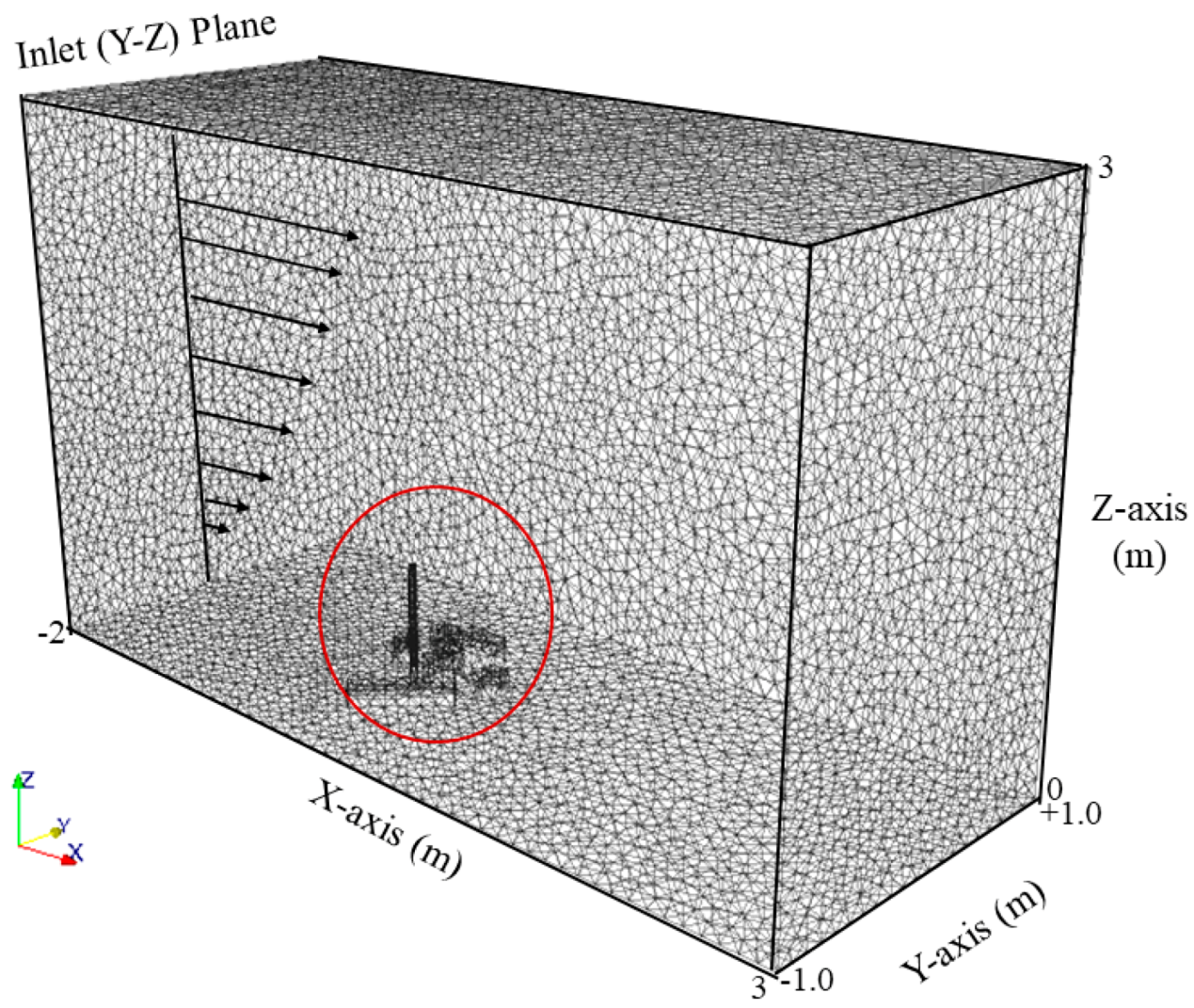
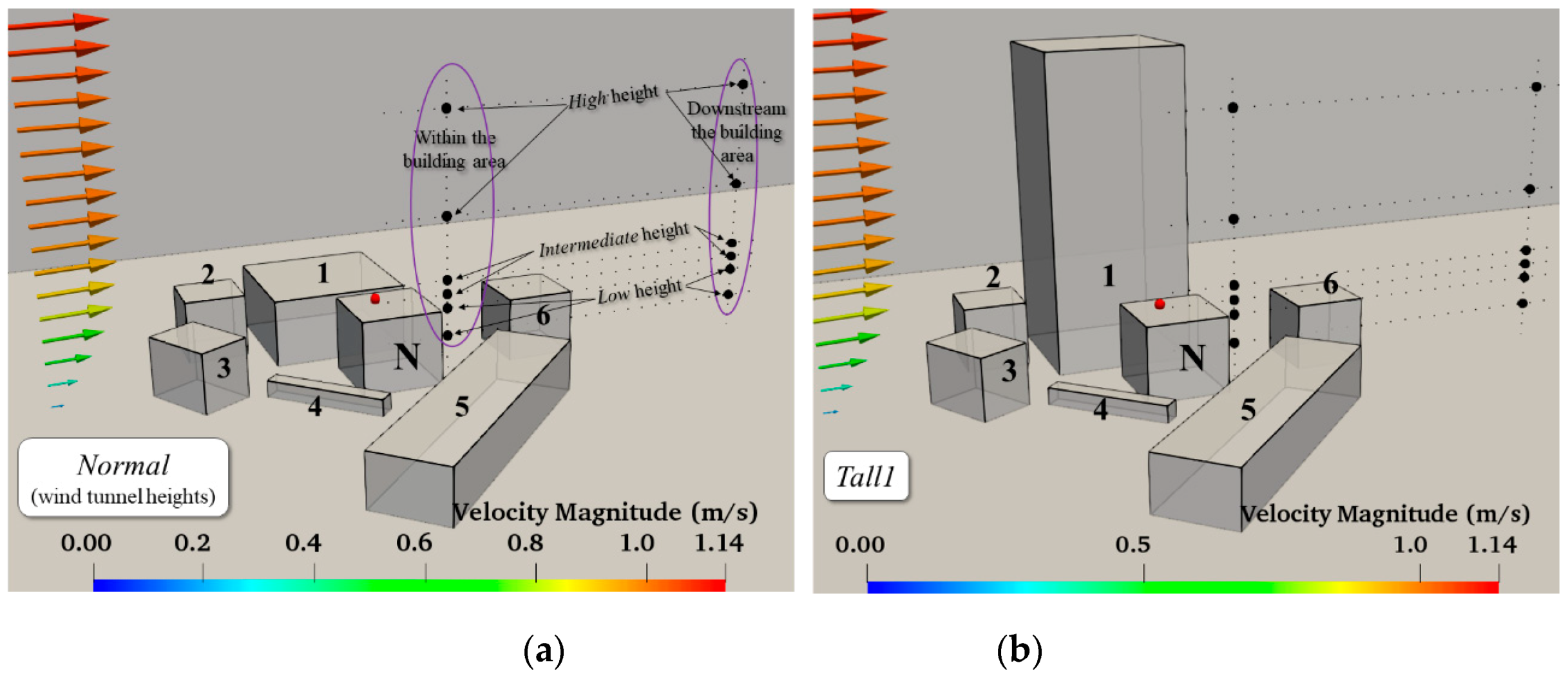
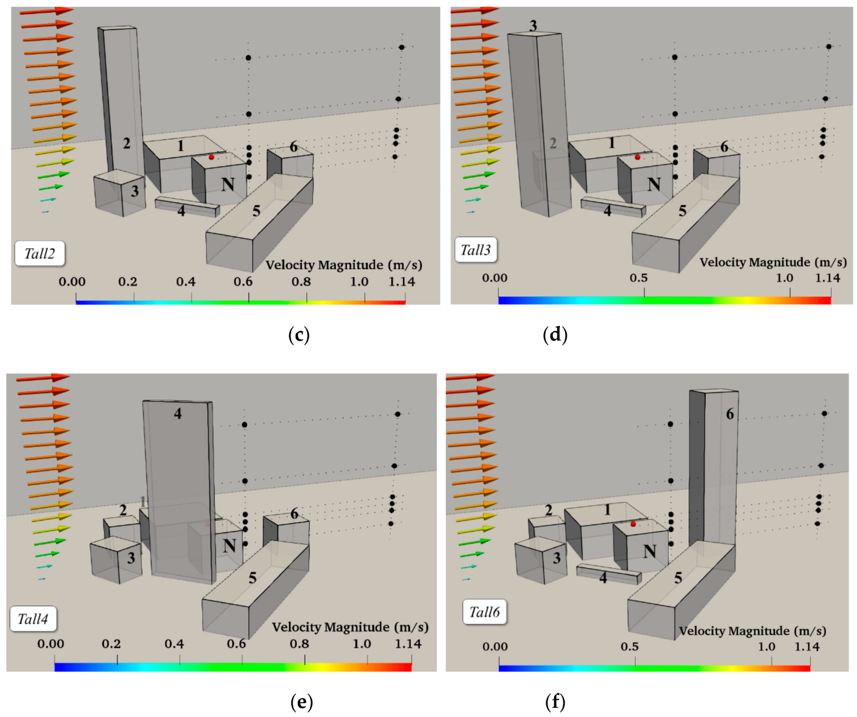
2.2. Computational Set-Up

The basic building configuration is shown in Figure 1, representing the wind tunnel set-up based on a 1:200 scaling [32].

Table 1. Building heights (m) for the different configurations.

Building	Wind Tunnel (Normal)	Tall1	Tall2	Tall3	Tall4	Tall6
N	0.1428	0.1428	0.1428	0.1428	0.1428	0.1428
1	0.1315	0.6	0.1315	0.1315	0.1315	0.1315
2	0.1238	0.1238	0.6	0.1238	0.1238	0.1238
3	0.1152	0.1152	0.1152	0.6	0.1152	0.1152
4	0.0315	0.0315	0.0315	0.0315	0.6	0.0315
6	0.1228	0.1228	0.1228	0.1228	0.1228	0.6

shows the height of the buildings in the wind tunnel case, together with the modified heights in each tall building configuration considered in the LES simulations, set to 0.6 m in the scaled version, corresponding to 120 m in real life. The tracer source is placed at the top left corner of the central building denoted as “N” at the height of Z = 0.1508 m, corresponding to a real height of 30.16 m, and it represents emissions from a Combined Heat and Power plant (CHP). As can be seen from the configurations (Figure 2), some buildings are downstream (east of) the source (Tall6), others upstream (Tall2 and Tall3, westerly), one north of the source (Tall1) and one building “south-westerly” of the source (Tall4). The dimensions of the computational domain were based on the wind tunnel building area and covered a volume of 5.0 m (length) by 2.0 m (width) by 3.0 m (height). The height of the domain was set to five times the height of the tallest building (0.6 m) as recommended by good CFD practice from urban flow simulations [26,33,34]. Moreover, the blockage ratio is equal to 2.3%, below the maximum value recommended of 3% [33,34]. The inflow wind is considered westerly with a mean velocity profile and mean Reynolds stresses, as measured in the wind tunnel, downstream the spires inlet and just outside the building area (Figure 3).

The synthetic eddy method of Jarrin et al. [35], as described in Pavlidis et al. [20], was subsequently implemented to generate the turbulent inlet boundary conditions on the left boundary of the domain. The downstream (easterly) boundary is the outlet and is by default a pressure boundary (no-stress condition). For the solid walls of the buildings and the “floor” of the domain, the no-slip condition was considered, whilst the slip and no-shear conditions were considered for the sides and top of the domain. The simulations were carried out in parallel (five processors being the optimal number of processors as explained in the mesh adaptivity section) on a standalone Dell multiprocessor, the Dell Precision Tower 7810 computer, with a dual Intel Xeon Processor. The simulations run for a time long enough to reach a statistically stationary, fully developed turbulent flow, with simulation times up to 45 s. Defining the ‘‘flow-through’’ as the time it would take a fluid particle to traverse the length of the domain (5 m long), this being typically 5 s, our simulation results are equivalent to 8/9 “flow-throughs”, a typical value for turbulent flow simulations. Time-averaging is computed by sampling the velocity field at the discrete locations, i.e., location of the detectors shown in Figure 2, and averaging the solution over the last 20 s of the simulation, ensuring the averaging is carried out after a statistically stationary fully turbulent flow has been achieved.

2.3. Mesh Adaptivity

The importance of adaptive, unstructured meshes [18] and the implementation of adaptive meshes for LES applications have already been highlighted [13]. This combination of LES computations and adaptivity/adaptive meshes is one of the innovative aspects of the FLUIDITY-LES software, as it allows remeshing of the domain based on a posteriori error estimates, whilst achieving certain targets for error. The process of adaptive remeshing consists of three parts: (i) deciding what mesh is desired, i.e., a coarser or a finer mesh; (ii) generation of this mesh; and (iii) transferring information to the latest mesh from the older one, based on a metric as chosen by the user (Fluidity manual, 2016). The process allows a number of actions to be taken such as: (i) reduction of the number of nodes and elements (corresponding to collapsing of edges), leading subsequently to coarsening of the mesh; the reverse, i.e., the increase of the number of nodes will result in a finer mesh; (ii) smoothing of the mesh by moving nodes whilst keeping the overall number of elements and nodes the same. As mentioned, the adaptivity within FLUIDITY is based on a posteriori error estimates, which aim at achieving certain targets for error, incorporating three options known as: (i) h-adaptivity (associated with mesh connectivity); (ii) p-adaptivity, linked with polynomial orders; and (iii) the r-adaptivity (associated with the relocation of element vertices). A combination of these can also be set, leading to the hr-adaptivity, which is what we implemented in this study. Adaptivity can be field-specific, i.e., different computed fields can be configured with their own specific adaptivity options. For our study, we carried out the adaptivity based on the velocity and concentration variables, setting interpolation errors for these variables. Mesh resolution was also controlled by specifying the maximum/minimum sizes of the elements, at different areas within the domain, with the element-minimum value being 0.003 m near the source location. Adaptivity was set to take place every 10 timesteps, with an adaptive time-step controlled by a CFL number of 0.9. The maximum number of nodes was set to 400,000 nodes per processor, allowing approximately 2 million elements for the whole domain. The initial mesh used at the very start of the simulation is shown in Figure 1. It consists of approximately 50, 20 and 30 elements in the x-, y- and z-directions, respectively, rendering a total number of nodes and elements in the initial mesh equal to 24,972 and 147,922, respectively. This mesh is only used at the start of the simulation and is then modified during the adaptivity process. Based on the scaling of the FLUIDITY software, the optimal number of nodes on each processor is estimated to be approximately equal to 80,000. The maximum number of nodes per process was set to 400,000 nodes, thus resulting in the equivalent and most appropriate number of processors being five processors. An example of the adaptivity effect on the computational mesh can be seen in Figure 4 for the instantaneous velocity and tracer fields for (a) Tall6 and (b) Tall3 configurations. In Figure 4, the mesh refinement can be clearly seen following the complex flows around the buildings and particularly in the wake generated by the taller building (Figure 4a), as well as the tracer dispersion (Figure 4b). This automatic refinement allows/ensures the accurate capturing of the turbulent flow behaviour as well as the pollution spread.

3. The LES Results

The purpose of this study was to carry out numerical experiments to assess the effect of the location of a tall building on the surrounding area in terms of air flow turbulence and dispersion of pollution. The main questions we wanted to address were: (a) are we able to see the effect of the location of a tall building on turbulence parameters and pollution concentrations? (b) Could we correlate the mean velocities and turbulence parameters with the pollution concentrations at different points in the domain? The analysis of our results consists of: (i) time-series plots of velocity magnitudes (Section 3.2); (ii) mean velocity magnitudes and mean concentrations (Section 3.3); it is to be noted that throughout the text, whenever velocities are mentioned, these refer to the velocity magnitudes; (iii) mean resolved Reynolds stresses (Section 3.4); (iv) mean turbulent kinetic energies (Section 3.5); and finally, (v) correlation analysis between variables using a statistical package (Section 3.6). Prior to the presentation of the results, we make a brief reference to the validation study carried out previously [32].

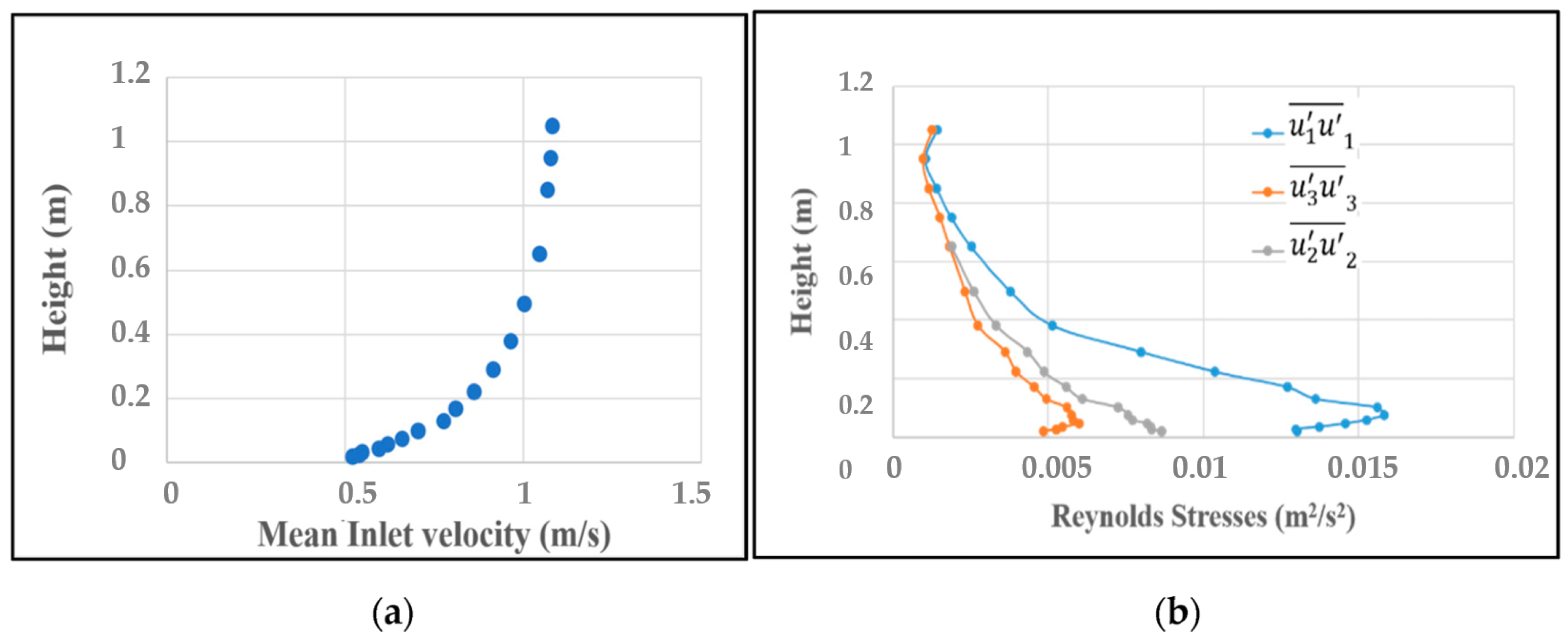
3.1. The Initial Validation

The validation work for our initial (referred to as normal) computational set-up was carried out and presented in our 2018 study [32], validating the simulations of the wind tunnel representation of the seven buildings’ (normal) configuration with wind tunnel data. The data was provided by Robins (personal communication) [36] following experiments in the 1:200 scale EnFlo wind tunnel (https://www.surrey.ac.uk/mes/research/aef/enflo/) with a fully developed, 1 m deep, simulated atmospheric boundary layer and dispersion experiments, using a reference wind velocity U_ref of 2.1 m/s, taken to be the air speed at the edge of the boundary layer. The simulated atmospheric boundary layer represented near-neutral atmospheric conditions and was initiated by a set of Irwin spires (vorticity-generators) at the inlet to the wind tunnel working section. The surface roughness condition was maintained by the roughness elements on the floor. The surface roughness length was 1.5 mm and the friction velocity 0.057Uref [37,38]. In these experiments, a passive tracer was released from the top left corner of the central building (Figure 1a), Building N, known as the Garden building), and measurements were taken for varying wind directions and model configurations. The source height was 0.1508 m, relative to the Garden building height of 0.143 m. Mean tracer concentrations were measured using Combustion Fast Flame Ionisation Detectors (FFIDs) carried on a three-dimensional traverse system. Our validation exercise was based on the comparison of the mean concentration data for one wind direction, with the LES simulation results with three different inlet boundary conditions. Differences ranged between 3% and 37%, with higher inconsistencies (>50%) exhibited in certain detector locations at low heights. More recently we implemented a data assimilation approach to investigate as to how the LES simulation results could be improved [39]. The implementation of the data assimilation method showed that the mean squared difference between the LES-FLUIDITY simulations and wind tunnel measurements can be reduced up to three order of magnitudes. In this current work, we utilise the seven buildings configuration and present an in-depth quantitative analysis of the effect of a tall building in their vicinity for tracer dispersion. The overall aim is to get a quantitative measure of how the presence of a tall building can affect the local mean flow and turbulence (turbulent fluctuations/Reynolds stresses) and their impact on the pollution dispersion. Two primary areas within the domain were chosen: (i) detectors within the building area and close to the source location, and (ii) detectors away from and downstream the building area, at a distance away and downstream the source. Distinct features are observed.

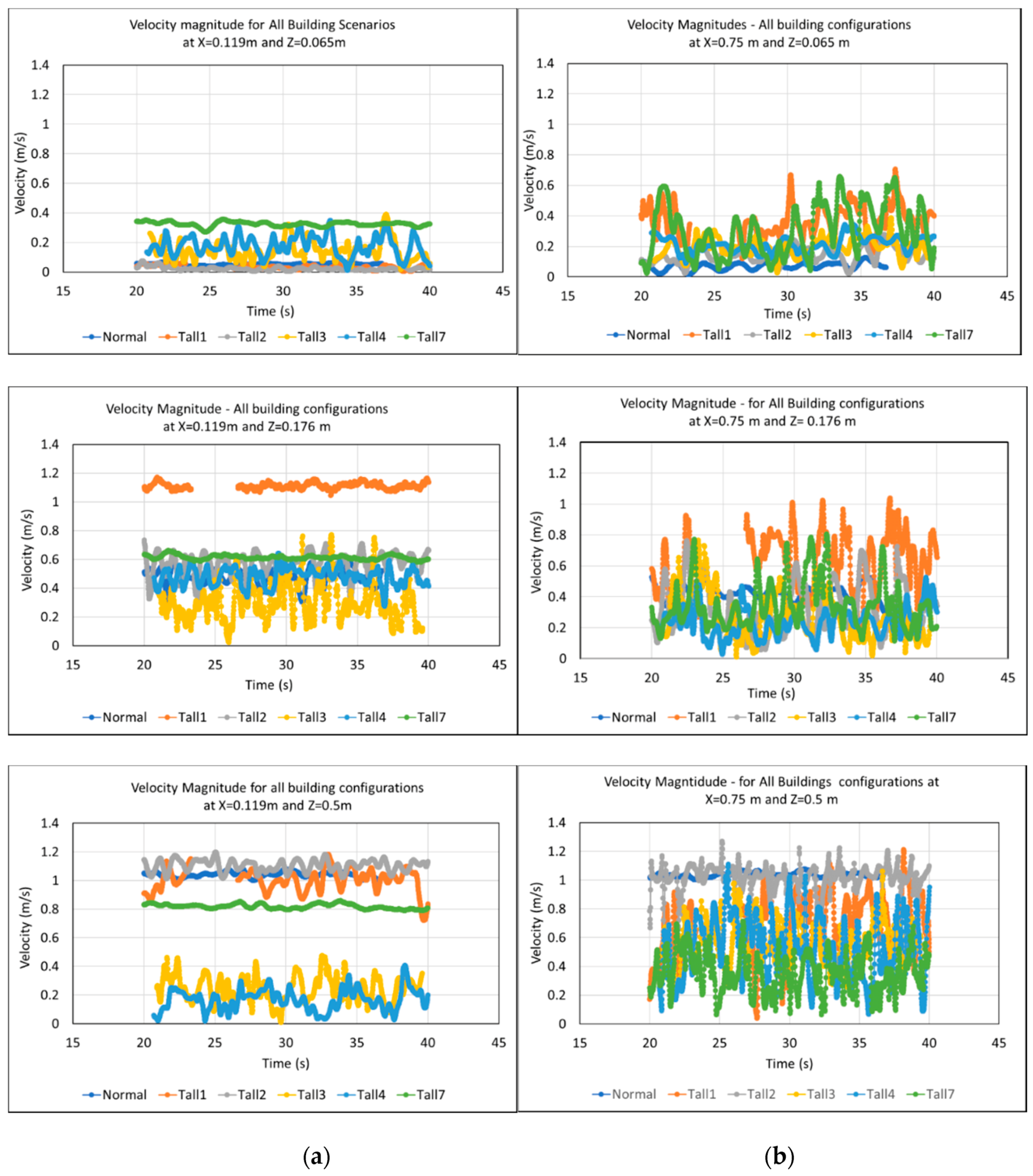
3.2. Time-Series of Velocity Magnitudes

Figure 5 shows the time-variation of the velocity magnitudes for the different configurations, at three different heights for the two main locations: (a) within the building area (X = 0.119 m, Y = 0.0 m) and (b) downstream the building area (X = 0.75 m, Y = 0.0 m). The aim was to ensure that a statistically steady-state turbulent flow has been achieved, and also to get an initial understanding of how the location of the tall building affected the time-series results. For the detectors within the building area, at the low height of Z = 0.065 m, the Tall6-configuration has the greatest effect, increasing the velocity.

Magnitudes relative to the normal set-up (N-configuration), whilst the Tall3 and Tall4 configurations, although they still increase the velocities at that location, they do this to a lesser extent. Configurations Tall1 and Tall2 yield velocities very similar to the N-configuration. However, at the higher level, Z = 0.5 m (still at X = 0.119 m, Y = 0.0 m, recall: the tallest building has a height of 0.6 m, hence the detector location is below the height of the tallest building), configuration Tall6 causes a reduction to the velocities, with configurations Tall3 and Tall4 causing even greater reductions relative to the N-configuration. Tall1 and Tall2 configurations seem to result in similar velocities as the N-configuration, at both heights, for the location within the building area. However, at the downstream location (X = 0.75 m, Y = 0.0 m) at the low levels (Z = 0.065 m), all configurations seem to yield velocity magnitude values higher than the N-configuration, with the Tall1-configuration yielding the greatest increase in velocities, followed by the Tall6-configuration. At the higher level (Z = 0.5 m), all configurations seem to decrease the velocities, relative to the N-configuration, except the Tall2-configuration, which results in velocity values very similar to the N-configuration. The greatest decrease is observed with the Tall6-configuration. These velocity magnitude reductions at the downstream location, although with different building configuration, is consistent with findings in the literature [40] who noted that the city’s breathability at downstream locations is reduced by the taller buildings upstream. How these variations are reflected in the time-averaged mean velocity values and in the mean concentrations, as well as the mean Reynolds stresses and turbulent kinetic energies (TKEs) are shown in Section 3.3, Section 3.4 and Section 3.5. Correlation coefficients between the various parameters, i.e., how velocities at one location are correlated with concentrations at the same location are presented, as well as how concentrations at one location are correlated with concentrations at another location are presented in Section 4.2.

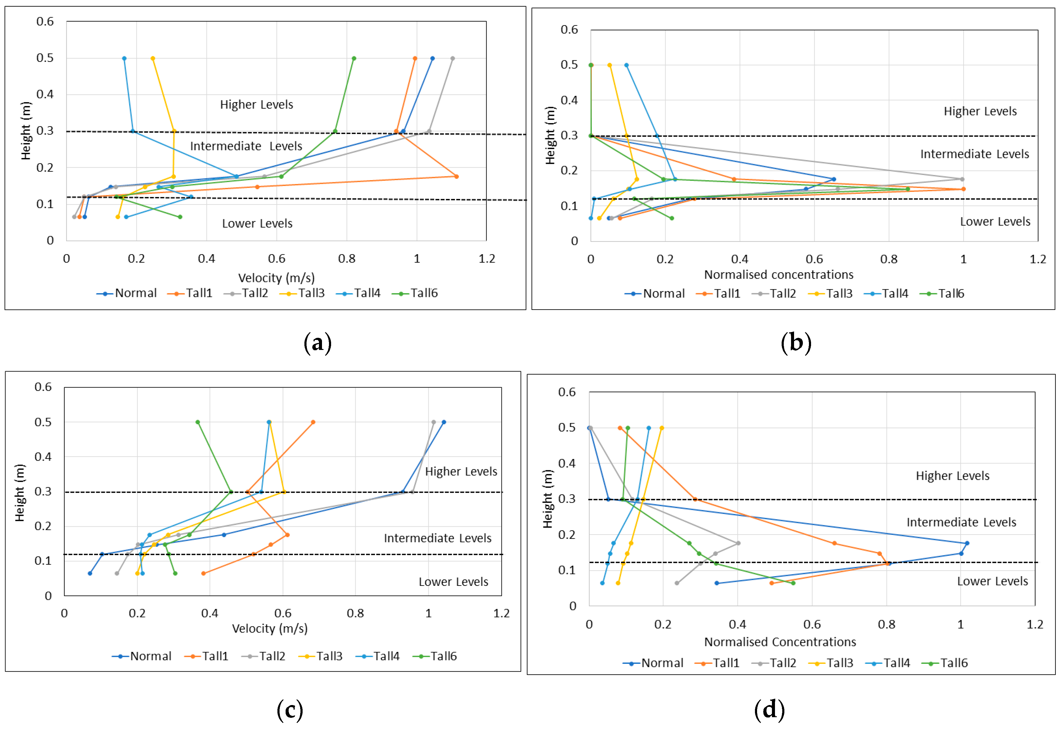
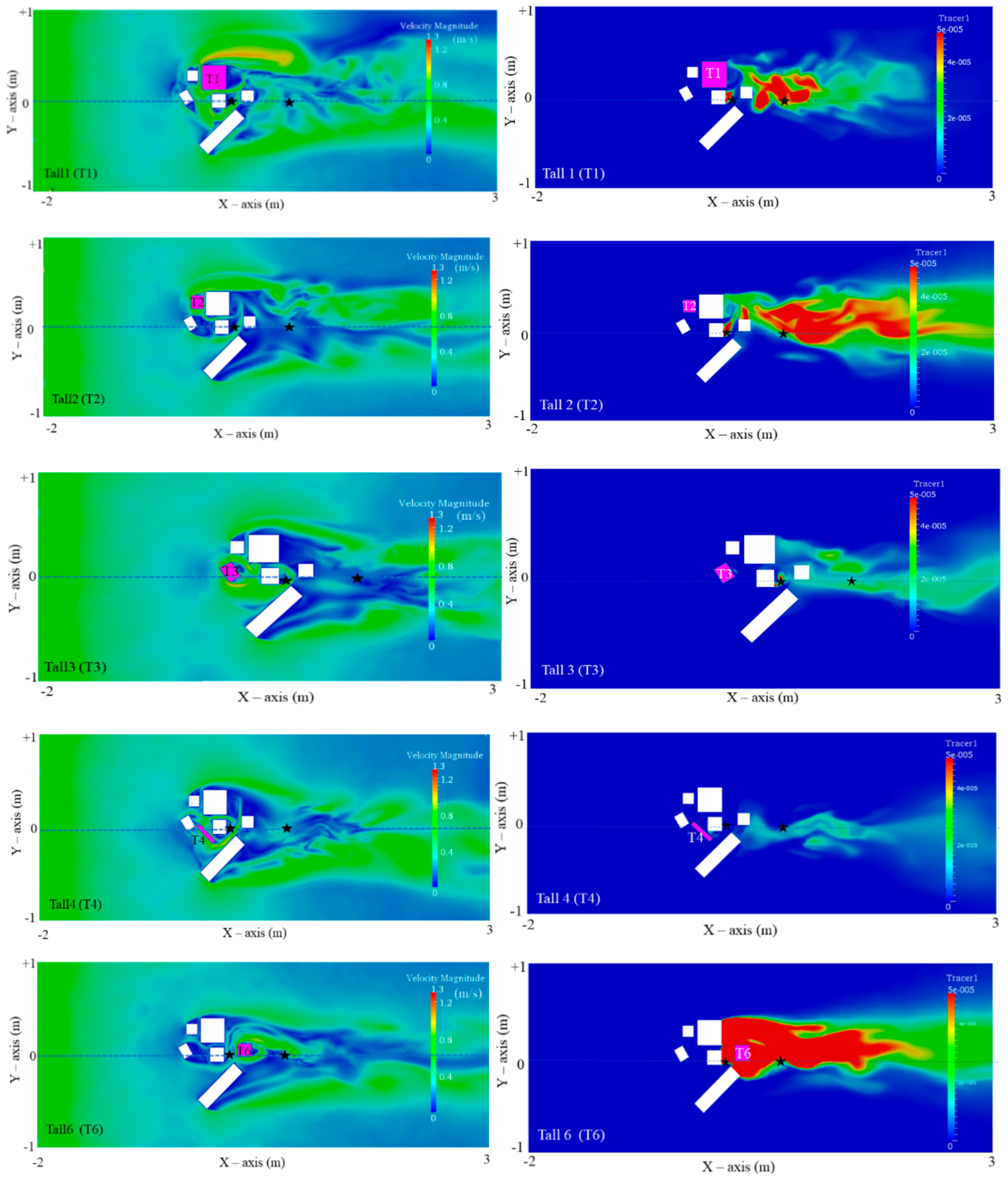
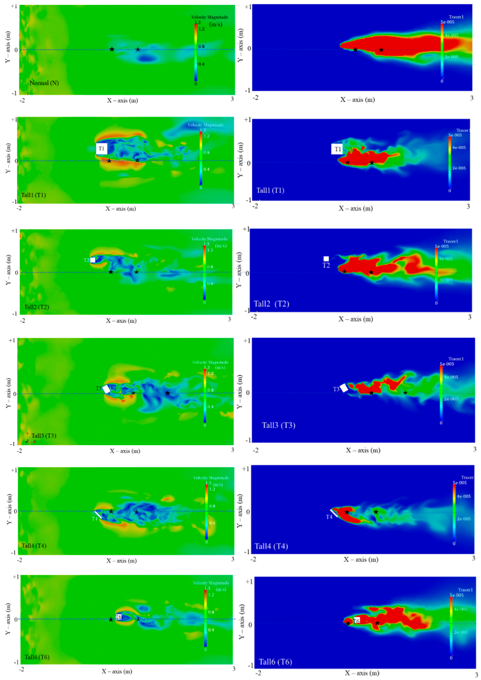
3.3. Mean Velocities and Concentrations

The variations of the mean velocity magnitudes and concentrations for all building configurations relative to the N-configuration, within the two primary areas (within and downstream the buildings) at different heights, are shown in Figure 6. We identify three main height levels at which distinct variations occur: (i) lower levels for heights below 0.12 m; (ii) intermediate levels for levels up to 0.3 m (specific detector locations at 0.148 m and 0.176 m), and (iii) higher levels for heights from 0.3 m and higher. In conjunction with the percentages changes in

Table 2. Percentage (%) change of mean velocities at two locations at varying heights.

Within the Building Area (X = 0.119 m, Y = 0.0 m)
Building Configuration	Z = 0.065 m	Z = 0.12 m	Z = 0.148 m	Z = 0.176 m	Z = 0.3 m	Z = 0.5 m
Tall 1	−29	−20	329	130	−2	−5
Tall 2	−58	−21	11	16	8	5
Tall 3	184	154	77	−37	−68	−76
Tall 4	232	462	108	0.11	−80	−84
Tall 6	528	125	138	27	−20	−22
Downstream area (X = 0.75 m, Y = 0.0 m)
Tall 1	451	400	124	40	−46	−34
Tall 2	109	68	−20	−29	3	−3
Tall 3	189	111	−3	−35	−35	−46
Tall 4	209	101	−16	−46	−42	−46
Tall 6	340	175	9	−22	−51	−65

Colour scheme: yellow shows increases; blue shows decreases.

and

Table 3. Percentage (%) change of mean concentrations at two locations at varying heights.

Within the Building Area (X = 0.119 m, Y = 0.0 m)
Building Configuration	Z = 0.065 m	Z = 0.12 m	Z = 0.148 m	Z = 0.176 m	Z = 0.3 m	Z = 0.5 m
Tall 1	59	5	73	−41	2173	1,117,771
Tall 2	15	−38	15	53	329	992
Tall 3	−53	−77	−83	−81	151,927	37,218,926
Tall 4	−99	−97	−82	−65	281,719	69,114,350
Tall 6	339	−56	47	−70	432	2086
Downstream the building area (X = 0.75 m, Y = 0.0 m)
Tall 1	43	−1	−22	−35	448	11,032
Tall 2	−31	−63	−65	−61	123	488
Tall 3	−77	−89	−90	−89	180	25,936
Tall 4	−89	−94	−94	−94	150	21,367
Tall 6	60	−58	−70	−74	75	13,695

Colour scheme: yellow shows increases; blue shows decreases.

, the results are summarised further below. Figure 7 and Figure 8 also present the 2D spatial variation of the velocities and pollution dispersion within the domain, at the specific heights of Z = 0.065 m and Z = 0.176 m, for all building configurations. Figure 7 and Figure 8 show the effect in horizontal planes, at two different height, for both the velocity magnitude and concentrations; however, it is important to also visually see the effect in a 3D space, and thus, Figure 9 shows both velocity streamlines as well as the tracer isosurface equal to 1 × 10⁻⁴ for the different configurations, clearly seeing the effect of the location of a tall building in the spread of pollution. We can clearly visually see the effect of each building configuration on the spread of the pollution and get an appreciation as to how the location of each tall building impacts the local environment. A more quantitative analysis is given in Section 3.5 further below.

3.4. Mean Resolved Reynolds Stresses

The principle of LES lies in the determination of the filtered/resolved flow, whilst the residual/unresolved flows are modelled using a subgrid-scale model, i.e., the large scales are directly numerically solved, whilst the smaller eddies are modelled using an empirical model. Considering the resolved velocity field, the time-averaged resolved velocities are estimated using the expression:

$$<{\tilde{\mathrm{u}}}_{\mathrm{i}}>=\left[\frac{1}{\mathrm{N}}{\displaystyle \sum }_{\mathrm{t}=1}^{\mathrm{N}}{\tilde{\mathrm{u}}}_{\mathrm{i}}\left(\mathrm{t}\right)\right]$$

(8)

where $\mathrm{N}$ is the total number of time-samples $\mathrm{t}$ in the time-series and $\mathrm{i}=\left\{1,2,3\right\}$ the space dimensions in the Cartesian coordinate system. The velocity fluctuation ${\mathrm{u}{}^{\prime }}_{\mathrm{i}}$ is then estimated using Equation (9):

$${ \mathrm{u}{}^{\prime }}_{\mathrm{i}}\left(\mathrm{t}\right)= {\tilde{\mathrm{u}}}_{\mathrm{i}}\left(\mathrm{t}\right)-<{\tilde{\mathrm{u}}}_{\mathrm{i}}>$$

(9)

The mean Reynolds stress tensor $\mathrm{Re}$, assuming a constant density, is defined as in Equation (10):

$$\mathrm{Re}=\overline{{\mathrm{u}{}^{\prime }}_{\mathrm{i}}{\mathrm{u}{}^{\prime }}_{\mathrm{j}}}=\frac{1}{\mathrm{N}}{\displaystyle \sum }_{\mathrm{t}=1}^{\mathrm{N}}{ \mathrm{u}{}^{\prime }}_{\mathrm{i}}\left(\mathrm{t}\right){ \mathrm{u}{}^{\prime }}_{\mathrm{j}}\left(\mathrm{t}\right)$$

(10)

where $\mathrm{i}$ and $\mathrm{j}$ are the space dimensions $\left\{\mathrm{x},\mathrm{y},\mathrm{z}\right\}$ in the Cartesian coordinates. The velocity components in the $\left\{\mathrm{x},\mathrm{y},\mathrm{z}\right\}$ directions are denoted by the letters $\left\{\mathrm{u},\mathrm{v},\mathrm{w}\right\}$, respectively. Figure 10 and Figure 11 present how both the nondiagonal components (i.e., $\overline{ \mathrm{u}{}^{\prime } \mathrm{v}{}^{\prime }}$, $\overline{ \mathrm{u}{}^{\prime } \mathrm{w}{}^{\prime }}$ and $\overline{ \mathrm{v}{}^{\prime } \mathrm{w}{}^{\prime }}$ ), and the diagonal components ($\overline{ \mathrm{u}{}^{\prime } \mathrm{u}{}^{\prime }}$, $\overline{ \mathrm{v}{}^{\prime } \mathrm{v}{}^{\prime }}$ and $\overline{ \mathrm{w}{}^{\prime } \mathrm{w}{}^{\prime }}$, for comparison reasons) vary with height Z, for all building configurations, at the two locations (X = 0.119 m, Y = 0.0 m) and (X = 0.75 m, Y = 0.0 m). The percentage changes for the nondiagonal components for all configurations (relative to the normal configuration) are shown in

Table 4. Percentage (%) change of the mean Reynolds stress components.

Within the Building Area (X = 0.119 m, Y = 0.0 m)
Building Configuration	Z = 0.065 m	Z = 0.12 m	Z = 0.148 m	Z = 0.176 m	Z = 0.3 m	Z = 0.5 m
$\left(i\right) \overline{u^{\prime }{u}^{\prime }}$
Tall 1	−41	−19	326	−92	1101	1377
Tall 2	−46	−50	185	76	107	230
Tall 3	5564	1350	885	396	6743	3904
Tall 4	2642	1048	1986	−23	3977	1254
Tall 6	−17	−85	−47	−95	−8	−46
$\left(ii\right) \overline{v^{\prime }{v}^{\prime }}$
Tall 1	136	298	156	−65	−44	10
Tall 2	4034	1040	7110	5894	1391	4498
Tall 3	6825	3119	5699	6344	16,007	2906
Tall 4	3487	1494	1957	145	3237	1102
Tall 6	−25	−4	−60	−87	−36	−63
$\left(iii\right) \overline{w^{\prime }{w}^{\prime }}$
Tall 1	414	163	196	185	243	72
Tall 2	142	140	130	384	121	−0.33
Tall 3	14,492	15,580	14,244	22,072	19,389	6205
Tall 4	5817	5983	3499	4441	15,721	5083
Tall 6	504	1367	38	−57	−33	−53
$\left(iv\right) \overline{u^{\prime }{v}^{\prime }}$
Tall 1	−99	269	−19,292	75	3755	88,009
Tall 2	−175	−112	28,594	1370	−683	10,987
Tall 3	2091	2813	64,533	9526	256,272	50,885
Tall 4	2896	−377	9504	−79	19,210	−64,635
Tall 6	−59	−92	541	85	−498	1908
$\left(v\right) \left(i\right) \overline{u^{\prime }{w}^{\prime }}$
Tall 1	79	174	−311	90	4053	617
Tall 2	594	188	130	−102	2864	66
Tall 3	75,910	971	715	445	59,255	−1775
Tall 4	−33,815	1721	−1369	467	62,277	684
Tall 6	162	267	−7	93	−1299	64
$\left(vi\right) \overline{v^{\prime }{w}^{\prime }}$
Tall 1	−984	486	1266	2733	99	664
Tall 2	−248	95	253	6288	2108	−824
Tall 3	20,355	132	−18,835	−34,960	4977	3053
Tall 4	−17,606	4291	−5978	15,664	110,571	15,657
Tall 6	486	1607	−175	−51	197	−112

and

Table 5. Percentage (%) change of mean nonisotropic Reynolds stresses.

Downstream the Building Area (X = 0.75m, Y = 0.0 m)
Building Configuration	Z = 0.065 m	Z = 0.12 m	Z = 0.148 m	Z = 0.176 m	Z = 0.3 m	Z = 0.5 m
$\left(i\right) \overline{u^{\prime }{v}^{\prime }}$
Tall 1	−1798	2384	3623	1567	65,784	1,477,173
Tall 2	−609	−1621	−2517	−565	905	253,283
Tall 3	196	−1199	−3647	−1000	8209	−125,944
Tall 4	−1815	−889	627	−144	−24,425	−1,251,768
Tall 6	−6752	−4886	−2341	561	25,347	277,463
$\left(ii\right) \overline{u^{\prime }{w}^{\prime }}$
Tall 1	−10,124	−1114	148	587	32,106	−26,815
Tall 2	374	−816	−602	−841	2136	131
Tall 3	−3783	−1455	−874	−987	−408	−5430
Tall 4	125	−293	−540	−825	−36,087	−11,894
Tall 6	13,069	2631	515	391	37,967	−5948
$\left(iii\right) \overline{v^{\prime }{w}^{\prime }}$
Tall 1	1636	2288	366	−5212	−6031	−34,895
Tall 2	−1533	209	209	236	478	1695
Tall 3	−2419	68	579	1006	4668	12,363
Tall 4	−93	−320	−140	−465	4021	819
Tall 6	−5112	−2123	−1679	−6197	−3521	−71,739

within the building area and downstream the building area, respectively, with the colour scheme being white for increases and blue for decreases. A more detailed analysis and discussion on the results are given in Section 4.

3.5. Turbulent Kinetic Energies (TKEs)

The mean turbulent kinetic energy (TKE) $\mathrm{k}$ is computed as shown in Equation (10):

$$\mathrm{k}=\frac{1}{2}{\displaystyle \sum }_{\mathrm{i}=1}^3\overline{{\mathrm{u}}_{\mathrm{i}}^{\prime }{}^2}$$

(11)

The variations of the mean TKEs for all configurations are shown in Table 2, for the two locations (within the building area and downstream the building area) at three heights: at the lower height (Z = 0.065 m), at intermediate height (Z = 0.176 m) and at higher height (Z = 0.5 m).

It is interesting to see the increased mean TKEs for almost all cases, relative to the normal configuration (tens of thousands of factors in some cases at the higher levels), with single exceptions as highlighted (in blue,

Table 6. Percentage (%) change of mean turbulent kinetic energies (TKEs) relative to the normal case.

Location	X = 0.119 m, Y = 0.0 m			X = 0.75 m, Y = 0.0 m
Building Configuration	Z = 0.065 m	Z = 0.176 m	Z = 0.5 m	Z = 0.065 m	Z = 0.176 m	Z = 0.5 m
Tall 1	79	−84	630	2521	1943	23,905
Tall 2	118	132	250	650	939	3824
Tall 3	7234	1375	4105	1530	1296	12,237
Tall 4	3357	74	2082	1425	937	25,447
Tall 6	42	−94	−53	4392	1144	19,944

Pink for positive (increase) and Blue for negative (decrease) values.

). The highly increased TKEs are specifically noticeable at the downstream location (X = 0.75 m, Y = 0.0 m). The question we wanted to address was as to how the increased TKEs impacted the mean tracer concentrations at the two locations at varying heights.

3.6. Correlation Coefficients

The Pearson correlation coefficient $\mathrm{r}$, ranging between −1 and 1, is a well-known way to measure the correlation between two variables and is computed as shown in Equation (12). Negative values indicate an inverse relationship between variables exists, i.e., if one variable increases the other variable decreases, whilst a positive correlation means that as one variable increases the other variable also increases. A value of 0 means there is no correlation between the variables.

$$\mathrm{r}=\frac{\mathrm{cov}\left(\mathrm{c},\mathrm{Y}\right)}{{\mathsf{\sigma }}_{\mathrm{c}}{\mathsf{\sigma }}_{\mathrm{Y}}}$$

(12)

In Equation (12), the $\mathrm{cov}\left(\mathrm{c},\mathrm{Y}\right)$ term is the covariance matrix of the variable $\mathrm{c}$ and the variable $\mathrm{Y}$. The variable c represents the tracer concentrations, whilst $\mathrm{Y}$ can represent either velocity magnitudes, or the Reynolds stresses, or the TKEs or the concentrations at a different location to the one for $\mathrm{c}$. The parameters ${\mathsf{\sigma }}_{\mathrm{c}}$ and ${\mathsf{\sigma }}_{\mathrm{Y}}$ are the standard deviation of the concentration $\mathrm{c}$ and the variable $\mathrm{Y}$, respectively. The IBM statistical software SPSS [41] was utilised to estimate the Pearson correlation coefficients for the tracer concentrations at specific locations in relation to: (a) the velocity values, the Reynolds stresses and the turbulent kinetic energy (TKE) at the same location and (b) the tracer concentrations at other locations. For the first analysis, we looked at how the tracer concentration at a specific point is correlated with the velocity, the Reynolds stresses, and TKE at the same point. We did this for two detector locations within the building area (same X and Y-coordinates but different heights), where: (i) X = 0.119 m, Y = 0.0 m, Z = 0.065 m; and (ii) X = 0.119 m, Y = 0.0 m, Z = 0.5 m.

For the second part of the analysis, we looked at how the tracer concentrations at the downstream location (X = 0.75 m, Y = 0.0 m) at height Z = 0.065 m are correlated with the concentrations at the upstream location (X = 0.119 m, Y = 0.0 m) within the building area at different heights. It was interesting to see how the correlation coefficients varied between the building configurations, and how the values changed in relation to the normal case. For example, for the normal case, the downstream concentrations at Z = 0.065 m correlated the strongest (positively) with the concentrations at X = 0.119 m, and Z = 0.12 m; however, when the tall buildings are considered, the strongest positive correlation (0.256) occurs for the Tall4 configuration with the concentrations at X = 0.119m and Z = 0.5m. The variation of all the correlation coefficients for each tall building configuration are shown in

Table 7. Pearson correlation coefficients between tracer concentrations and velocities, Reynolds stresses and TKEs at: X = 0.119 m, Y = 0 m, Z = 0.065 m.

Configuration	Vel	$\overline{{\mathit{u}}^{\prime }{\mathit{u}}^{\prime }}$	$\overline{{\mathit{v}}^{\prime }{\mathit{v}}^{\prime }}$	$\overline{{\mathit{w}}^{\prime }{\mathit{w}}^{\prime }}$	$\overline{{\mathit{u}}^{\prime }{\mathit{v}}^{\prime }}$	$\overline{{\mathit{u}}^{\prime }{\mathit{w}}^{\prime }}$	$\overline{{\mathit{v}}^{\prime }{\mathit{w}}^{\prime }}$	TKE
Normal	−0.041	−0.340	−0.074	0.002	−0.295	−0.118	−0.282	−0.307
Tall1	0.294	−0.265	0.044	0.119	0.200	−0.231	0.085	0.009
Tall2	−0.369	−0.183	−0.253	−0.049	0.231	0.080	0.212	−0.260
Tall3	−0.243	−0.001	−0.079	−0.066	−0.029	−0.074	−0.036	−0.069
Tall4	−0.537	0.101	0.199	0.262	0.299	−0.225	−0.133	0.256
Tall6	0.337	−0.198	0.050	−0.126	−0.250	−0.180	−0.205	−0.182

,

Table 8. Pearson correlation coefficients between tracer concentrations and velocities, Reynolds stresses and TKEs at: X = 0.119 m, Y = 0 m, Z = 0.5 m.

Configuration	Vel	$\overline{{\mathit{u}}^{\prime }{\mathit{u}}^{\prime }}$	$\overline{{\mathit{v}}^{\prime }{\mathit{v}}^{\prime }}$	$\overline{{\mathit{w}}^{\prime }{\mathit{w}}^{\prime }}$	$\overline{{\mathit{u}}^{\prime }{\mathit{v}}^{\prime }}\prime$	$\overline{{\mathit{u}}^{\prime }{\mathit{w}}^{\prime }}$	$\overline{{\mathit{v}}^{\prime }{\mathit{w}}^{\prime }}$	TKE
Normal	−0.198	0.003	−0.103	0.026	0.144	−0.041	−0.016	−0.043
Tall1	−0.875	0.371	0.116	0.372	0.026	0.372	0.145	0.388
Tall2	0.414	0.088	0.273	0.008	−0.220	−0.117	0.127	0.218
Tall3	−0.214	0.125	0.055	0.047	0.174	0.015	0.060	0.172
Tall4	0.228	0.030	0.228	0.174	0.084	−0.053	0.284	0.212
Tall6	0.011	0.011	0.079	−0.018	0.013	−0.064	−0.078	0.038

and

Table 9. Pearson correlation coefficients between tracer concentrations at the downstream location: X = 0.75 m, Y = 0.0 m, Z = 0.065 m, with tracer concentrations at the within the building area location: X = 0.119 m, Y = 0.0 m, at different heights.

Building Configuration	Z = 0.065 m	Z = 0.12 m	Z = 0.148 m	Z = 0.176 m	Z = 0.3 m	Z = 0.5 m
Normal	0.048	0.53	−0.184	−0.095	−0.071	n/a
Tall1	0.066	0.103	0.118	−0.029	0.01	0.036
Tall2	0.041	−0.326	−0.272	−0.231	0.077	−0.032
Tall3	0.008	0.038	0.1	0.124	0.199	0.067
Tall4	0.054	−0.057	0.149	−0.026	0.221	0.283
Tall6	−0.215	−0.294	0.077	−0.137	0.0318	0.075

.

4. Analysis and Discussion

4.1. Mean Velocity Magnitudes, Concentration, Reynolds Stresses and TKEs

In this section we combine the findings from the mean velocity, concentrations and Reynolds stresses results and offer possible interpretations.

4.1.1. Within the Building Area: (X = 0.119 m, Y = 0.0 m)

At low heights (Z = 0.065 m and Z = 0.12 m): The Tall4 and Tall6 configurations have the greatest effect in increasing the mean velocities, followed by Tall3. Tall2 has the greatest effect in decreasing the mean velocities. This clearly indicates the importance of the location of the tall building. Tall6 is downstream/east of the source building, whilst Tall4 is upstream but at an angle. Tall3 is also upstream and aligned with building N but a little bit far away. Mean concentrations decrease for the Tall3 and Tall4 (up to 99% decrease), whilst they increase substantially (by a factor of 339%) for the Tall6 configuration at the lowest height of Z = 0.065 m, acting as a barrier, leading to trapping the pollution at the very lower levels. The 2D plots in Figure 8 also show visually how the Tall3 and Tall4 configurations have an impact locally on the dispersion, in a horizontal plane, showing clearly the location and orientation of these two buildings have lowered the pollution concentrations. In Figure 8, we also see the impact of the Tall6 configuration, where pollution is trapped within the source buildings and the nearby buildings. Yet, slightly higher up, at Z = 0.12 m, the concentrations for the Tall6 configuration decrease by a factor of 56%, affected by the flow field at and turbulence at that level. At Z = 0.065 m, pollution concentrations were still high at the lower levels (Z = 0.065 m) despite the noticeable increase in TKEs for certain configurations (Table 6).

How do these observations relate to the changes in the mean Reynolds stresses, particularly the nondiagonal components? For these lower heights, we can clearly from Figure 9, the effect of the Tall3 and Tall4 configurations in increasing the mixing through the horizontal component $\overline{ \mathrm{u}{}^{\prime } \mathrm{v}{}^{\prime }}$ by per cent factors between 2000 and 3000 at the low heights (Z = 0.065 m) and even higher percentage changes at intermediate heights (Z = 0.148 m and Z = 0.176 m), with a 64,533% increase (Table 4) specifically for the Tall3 configuration at Z = 0.148 m, prominent in Figure 9. Configurations Tall1, Tall2 and Tall6 have a negative effect on $\overline{ \mathrm{u}{}^{\prime } \mathrm{v}{}^{\prime }}$, i.e., decreases by factors ranging between 50% and 200% (Table 4), but a positive effect (increase) on the $\overline{ \mathrm{u}{}^{\prime } \mathrm{w}{}^{\prime }}$ component, increasing its value in the range of 70% to 600%. The effect on the $\overline{ \mathrm{v}{}^{\prime } \mathrm{w}{}^{\prime }}$ component, for these three configurations (i.e., Tall1, Tall2, and Tall6) is a combination of decreases and increases, with Tall1 and Tall2 decreasing the $\overline{ \mathrm{v}{}^{\prime } \mathrm{w}{}^{\prime }}$ by factors in the range of 250% to 1000%, whilst Tall6 has a positive effect, increasing the $\overline{ \mathrm{v}{}^{\prime } \mathrm{w}{}^{\prime }}$ component by a factor of 486% (Table 4). The question is which Reynolds stress component dominates, as mean concentrations increase for these three configurations, at the lowest height of Z = 0.065 m. It seems that although the mixing component $\overline{ \mathrm{u}{}^{\prime } \mathrm{w}{}^{\prime }}$ increases for these configurations, the fact that the $\overline{ \mathrm{v}{}^{\prime } \mathrm{w}{}^{\prime }}$ component decreases by higher factors for Tall1 and Tall2 may be the reason for the higher concentrations for these configurations. However, the same is not true for the Tall6 configuration, since despite the substantial increase of the mixing components $\overline{ \mathrm{u}{}^{\prime } \mathrm{w}{}^{\prime }}$ and $\overline{ \mathrm{v}{}^{\prime } \mathrm{w}{}^{\prime }}$ (162% and 486%, respectively), the concentrations still increase. Could these be due to the decrease in the $\overline{ \mathrm{u}{}^{\prime } \mathrm{v}{}^{\prime }}$ (59% decrease)? The effect of the Tall6 building results in higher concentrations despite the increases in both the mean velocities and mixing Reynolds stresses at the low height.

At intermediate heights (Z = 0.148 m and Z = 0.176 m): All configurations lead to an increase of the mean velocities (except for Tall3 at height Z = 0.176 m). At Z = 0.148m, all configurations lead to an increase of mean velocities. Tall1 configuration has the greatest effect, increasing the velocities by a factor of 329% (Table 2), followed by the Tall6 and Tall4 configurations. However, as we can see from Figure 6 and Table 3, this does not mean an automatic reduction of mean concentrations. Only configurations Tall3 and Tall4 result in decreased mean concentrations, by very similar factors of 83% and 82%, respectively. The other configurations (Tall1, Tall2 and Tall6) led to increased mean concentrations at this level, despite the increased mean velocities, with the Tall1 configuration yielding the highest increase of 73%. Tall1 is directly north of the source building, whilst Tall2 is still north but further west, hence its impact considerably reduced. Tall6 is downstream (east of the source building), hence expecting it would prevent pollution from spreading downwards and resulting in a higher increase of 47%, although not as high as the Tall1 configuration.

What happens to the TKEs at these intermediate heights? From Table 6, we can see that at Z = 0.176 m, a decrease of TKEs is observed at that level for the Tall1 and Tall6 configurations. For the other configurations (Tall2, Tall3 and Tall4), there were high increases in TKEs; yet, only Tall3 and Tall4 configurations resulted in lower concentrations (Table 3). Could the mean concentrations be affected by the mixing components of the Reynolds stresses? How do the nondiagonal/mixing components of the Reynolds stresses influence the mean concentrations at this height (Z = 0.148 m)? From Table 4, the $\overline{ \mathrm{u}{}^{\prime } \mathrm{v}{}^{\prime }}$ component increases for all configurations, except for Tall1 for which a decrease of ~20,000% is observed. This may well be responsible for the highest increase in mean concentrations (by 73%, as stated above) for this configuration. All other configurations increase the $\overline{ \mathrm{u}{}^{\prime } \mathrm{v}{}^{\prime }}$ component, with Tall3 resulting in the highest increase. Looking at the effect of horizontal ($\overline{ \mathrm{u}{}^{\prime } \mathrm{v}{}^{\prime }}$ ) and vertical mixing ($\overline{ \mathrm{u}{}^{\prime } \mathrm{v}{}^{\prime }}$and $\overline{ \mathrm{v}{}^{\prime } \mathrm{w}{}^{\prime }}$) components on the mean concentrations, the Tall2 configuration shows increases in both; yet, the mean concentrations also increase, although with a smaller percentage increase of 15% (Table 3). Configurations Tall3 and Tall4 show increases in the horizontal mixing component ($\overline{ \mathrm{u}{}^{\prime } \mathrm{v}{}^{\prime }},$64,533% and 9504%, respectively) but decreases in the vertical mixing component $\overline{ \mathrm{v}{}^{\prime } \mathrm{w}{}^{\prime }}$ (18,835% and 5978% decreases, respectively); yet, the effect on the mean concentrations is to lower the concentrations, indicating perhaps that the enhanced horizontal mixing plays a greater effect in this case, as opposed to the reduced vertical mixing. Configuration Tall6 results in increased mean concentrations of 47%, despite the enhanced horizontal mixing, ($\overline{ \mathrm{u}{}^{\prime } \mathrm{v}{}^{\prime }}$ increases by 541%) and mean velocities (Table 2 and Table 3). In this case, the decrease in the vertical mixing ($\overline{ \mathrm{v}{}^{\prime } \mathrm{w}{}^{\prime }}$ decrease of 175%) may be responsible for the higher concentrations.

At the slightly higher level of Z = 0.176 m: all configurations led to an increase of mean velocities, except interestingly for the Tall3 configuration. Tall3 reduces the mean velocities by a factor of 37% at this height. At this height, there is a corresponding decrease in mean concentrations (Table 3, including Tall3), with the exception now of the Tall2 configuration. The mixing components of the Reynolds stresses vary also between configurations. The horizontal component increases for all configurations, except for configuration Tall4, where a reduction of 79% is observed. However, this seems to be compensated by the increases of the vertical mixing components $\overline{ \mathrm{u}{}^{\prime } \mathrm{w}{}^{\prime }}$ and $\overline{ \mathrm{v}{}^{\prime } \mathrm{w}{}^{\prime }}$(446% and 15,664%, respectively) and hence leading to effectively no change in the mean concentrations (0.11% in Table 3). For Tall2, despite the increases of the mean velocities by a factor of 16%, together with the increases of the horizontal mixing component of the Reynolds stresses ($\overline{ \mathrm{u}{}^{\prime } \mathrm{v}{}^{\prime })}$ by 1370%, and the vertical component $\overline{ \mathrm{v}{}^{\prime } \mathrm{w}{}^{\prime }}$by 6288%, the mean concentrations still increased by as much as 53% (Table 3). For this configuration, only the vertical mixing component $\overline{ \mathrm{u}{}^{\prime } \mathrm{w}{}^{\prime }}$ decreased by 102%. Could this be overwriting the effects of the other variables? Tall2 lies “north” of the source but further west (compared to Tall1) and yet its impact leads to increased concentrations at this higher level.

At higher heights (Z = 0.3 m and Z = 0.5 m): Interestingly, all configurations lead to decreases in the mean velocities, apart from the Tall2 configuration which leads to a slight increase of 8% relative to the N-configuration at Z = 0.3 m. The greatest decrease occurs with the Tall4 configuration, by factors 80% and 84% at Z = 0.3 m and Z = 0.5 m, respectively, followed by the Tall3 (by factors of 68% and 76% at Z = 0.3 m and Z = 0.5 m, respectively) and Tall6 configurations by factors close to 20% at both heights. At these higher levels, it is interesting to see concentrations increase for all configurations. Massive increases occur specifically for Tall3 and Tall4 configurations (buildings upstream of the source, Tall3 west of the source, and Tall4 south-westerly, at both heights, and these increases are consistent with the decreases in the mean velocities.

It is interesting to see at the higher levels (Z = 0.5 m) all configurations resulted in high tracer concentrations despite the high increases in TKEs (Table 6) at that level. Could this be explained by the lowering/reduction of the mean velocities at that level (Table 2, except for the Tall2 configuration)? Do the mixing components of the Reynolds stresses have a role to play? These observed concentration increases for all configurations seem to occur despite the increases observed in all of the mixing components of the Reynolds stresses, with some exceptions. From Table 4, for both the horizontal mixing component ($\overline{ \mathrm{u}{}^{\prime } \mathrm{v}{}^{\prime })}$ and the vertical mixing components (($\overline{ \mathrm{u}{}^{\prime } \mathrm{w}{}^{\prime })}$ and ($\overline{ \mathrm{v}{}^{\prime } \mathrm{w}{}^{\prime }))}$, we see increases ranging from 64% (Tall6 configuration at Z = 0.5 m) to 25,6252% (Tall3 configuration). Some exceptions occur, with reduced horizontal mixing ($\overline{ \mathrm{u}{}^{\prime } \mathrm{v}{}^{\prime })}$ for the Tall2 and Tall6 configurations at Z = 0.3 m (683% and 498%, respectively) and the Tall4 configuration at Z = 0.5 m (64,635% reduction); reductions in the vertical mixing component ($\overline{ \mathrm{u}{}^{\prime } \mathrm{w}{}^{\prime })}$ are observed for the Tall6 configuration at Z = 0.3 m (1299% decrease); however, the vertical mixing component $\overline{\left( \mathrm{v}{}^{\prime } \mathrm{w}{}^{\prime }\right)}$ increases by 197% for Tall6 at that height. The Tall3 configuration at Z = 0.5 m results in a reduction of 1775% of the ($\overline{ \mathrm{u}{}^{\prime } \mathrm{w}{}^{\prime })}$ component; however, for the same configuration, the horizontal mixing ($\overline{ \mathrm{u}{}^{\prime } \mathrm{v}{}^{\prime })}$ has increased by 50,885% at Z = 0.5 m, and so has the vertical mixing component $\overline{\left( \mathrm{v}{}^{\prime } \mathrm{w}{}^{\prime }\right)}$ by 3053%.

The vertical mixing component $\overline{\left( \mathrm{v}{}^{\prime } \mathrm{w}{}^{\prime }\right)}$ increases for all configurations at the height of Z = 0.3 m, whilst for the Z = 0.5 m height, it decreases for the Tall2 and Tall6 configurations (824% and 112% decreases, respectively. However, despite the reduction in the vertical component, these configurations have high increases in the horizontal mixing component (10,987% for the Tall2 configuration and 1908% for Tall6).

4.1.2. Downstream the Building Area (X = 0.75 m, Y = 0.0 m, Tables 2 and 3)

At low heights (Z = 0.065 m and Z = 0.12 m): At Z = 0.065 m, all configurations increase the mean velocities, with Tall1 having the greatest effect (by factor 451%), followed by Tall6, Tall4 and Tall3. Table 3 shows a decrease of concentrations for configurations Tall2, Tall3, and Tall4, all these buildings are upstream of the source. However, mean concentrations for Tall1 (north of the source) and Tall6 (east of the source) configurations increase by factors of 43% and 60%, respectively, despite the increased mean velocities and the increased TKEs by hundreds/thousands of factors (Table 6), for all configurations.

Could the mixing components of the Reynolds stresses have a role to play here? From Table 4 and Table 5, for the Tall1 configuration, there is a reduction of the horizontal mixing component $\overline{ \mathrm{u}{}^{\prime } \mathrm{v}{}^{\prime }}$ nearly 1800% (1798%), and a decrease of 6752% for the Tall6 configuration (as opposed to 59% reduction at X = 0.119 m). Could these reductions in the horizontal mixing be responsible for the increased concentrations at that height for the Tall1 and Tall6 configurations, increases of 43% and 60%, respectively, as indicated earlier (Table 3)? For the Tall4 configuration, there is even a considerable reduction of $\overline{ \mathrm{u}{}^{\prime } \mathrm{v}{}^{\prime }}$ by nearly 2000 (1815%); yet, the mean concentrations here are reduced by 89%, a similar value to the 99% decrease at X = 0.119 m. The Tall4 configuration is associated, at X = 0.75 m, with an increase of 125% for the $\overline{ \mathrm{u}{}^{\prime } \mathrm{w}{}^{\prime }}$ and a (relatively small) reduction of 93% of the $\mathrm{v}{}^{\prime } \mathrm{w}{}^{\prime }$ component. Could the increase of 125% for the $\overline{ \mathrm{u}{}^{\prime } \mathrm{w}{}^{\prime }}$ component be also responsible for the reduced concentrations for the Tall4 configuration? Or is the combination with the increased mean velocity (209% increase) that leads to the reduced values? At the higher level of Z = 0.12 m, mean concentrations decrease for all configurations, with the greatest decrease (94%) occurring for Tall4 configuration. This may be explained with the corresponding increases in the mean velocities at that level, increases that range from 68% for the Tall2 configuration, to 400% for the Tall1 configuration (Table 2). It is interesting to see that although for the Tall1 configuration, the horizontal and vertical mixing components, $\overline{ \mathrm{u}{}^{\prime } \mathrm{v}{}^{\prime }}$ and $\overline{ \mathrm{v}{}^{\prime } \mathrm{w}{}^{\prime }}$ increase by 2394% and 2288%, respectively, as well as the increased mean velocity by 400% (Table 2), the mean concentrations only decrease very slightly, by 1%. For the Tall2 configuration, the mixing components of the Reynolds stress have decreased at that height, for this downstream location, by factors of 1621% for the $\overline{ \mathrm{u}{}^{\prime } \mathrm{v}{}^{\prime }}$ component, 816% for the $\overline{ \mathrm{u}{}^{\prime } \mathrm{w}{}^{\prime }}$, whilst the vertical mixing component $\overline{ \mathrm{v}{}^{\prime } \mathrm{w}{}^{\prime }}$ increased by 209%. Despite the decreased mixing components of the Reynolds stress, mean concentrations still decreased, indicating that perhaps the increased mean velocities had a greater effect at that height.

At intermediate heights (Z = 0.148 m and Z = 0.176 m): All mean concentrations decrease (Table 3), with the Tall4 configuration showing the largest decrease of 94% followed by Tall3 and Tall6, while the velocity changes are a mixture of increases (124% and 40% for the Tall1 configuration and 9% for Tall6 at Z = 0.148 m) and decreases for all other configurations. How do these relate to the changes in the TKEs and Reynolds stress components? From Table 5, we can see that the Tall1 configuration leads to increases in all three mixing components ($\overline{ \mathrm{u}{}^{\prime } \mathrm{v}{}^{\prime }}, \overline{ \mathrm{u}{}^{\prime } \mathrm{w}{}^{\prime }}$, and $\overline{ \mathrm{v}{}^{\prime } \mathrm{w}{}^{\prime }})$ (3623%, 148% and 366%) at Z = 0.148 m, with a reduction in the mean concentrations by 22%. For the same configuration, at the higher level of Z = 0.176 m, the mean concentrations are reduced by 35%, despite the reduction of the vertical mixing component $\mathrm{v}{}^{\prime } \mathrm{w}{}^{\prime }$ by 5212%. Thus, the reduction of the mean concentration here may be attributed to the enhanced horizontal mixing ($\overline{ \mathrm{u}{}^{\prime } \mathrm{v}{}^{\prime }},$) as well as the increased mean velocity by 40%. For all other configurations, at Z = 0.176 m, the mean velocities are reduced, and similarly, all mean concentrations are reduced. Could these reductions in the mean concentrations be related to enhanced mixing? Table 5 shows that at this downstream location, at Z = 0.176 m, for configurations Tall2, Tall3 and Tall4, the mixing components $\overline{ \mathrm{u}{}^{\prime } \mathrm{v}{}^{\prime }}, \mathrm{and} \overline{ \mathrm{u}{}^{\prime } \mathrm{w}{}^{\prime }}$ reduce substantially, with reduction values from 144% to 1000%. Only the vertical mixing component,$\overline{ \mathrm{v}{}^{\prime } \mathrm{w}{}^{\prime }})$, increases for the Tall2 and Tall3 configurations (236% and 1006%, respectively), whilst for the Tall4 configuration, there is a reduction by 465%. Thus, it is unclear as to what might be causing the reduction of mean concentrations for the Tall4 configuration, since both the mean velocities as well as the mixing components of the Reynolds stress are also reduced at that point.

Having said this, all configurations at Z = 0.176 m show increased TKEs by hundreds/thousands of factors (Table 6) at this height, and it is interesting to see that for all configurations (no exceptions) the mean concentrations are also reduced (Table 3), despite reductions in mean velocities for some configurations (Table 2) and reductions in some of the mixing (nondiagonal) components of the Reynolds stresses. Thus, the increased TKEs at these levels is consistent with the reduced concentrations.

At higher heights (Z = 0.3 m and Z = 0.5 m): Equally perplexing and interesting findings, to the ones at the intermediate heights, are observed at the higher levels from Z = 0.3 m and higher. It is clearly seen from Table 3 that all mean concentrations, for all configurations, at these higher levels are increased, with the highest increase occurring for the Tall3 configuration at Z = 0.5 m. It is equally observed that at both heights, all configurations lead to a decrease in the mean velocities, except the Tall2 configuration, which leads to a very slight increase of 3% when the height is Z = 0.3 m. The greatest decrease is caused by the Tall6 configuration at Z = 0.5 m. How are the Reynolds stress mixing components, $\overline{ \mathrm{u}{}^{\prime } \mathrm{v}{}^{\prime }, }\overline{ \mathrm{u}{}^{\prime } \mathrm{w}{}^{\prime }}$ and $\overline{ \mathrm{v}{}^{\prime } \mathrm{w}{}^{\prime }}$ behave at these heights? Again, Table 5 shows a mixture of increases and decreases, with massive/huge increases for the horizontal mixing component $\overline{ \mathrm{u}{}^{\prime } \mathrm{v}{}^{\prime }, }$ for the Tall1, Tall2 and Tall6 configurations, with values as high as 1,477,173% increase, whilst there are massive reductions for the Tall3 and Tall4 configurations at Z = 0.5 m. Interestingly, for the Tall2, Tall3 and Tall4 configurations, there are considerable increases in the vertical mixing component, $\mathrm{v}{}^{\prime } \mathrm{w}{}^{\prime }$, at both heights, with increases ranging from 478% for the Tall2 configuration, to 12,363% for the Tall3 configuration. Yet, these increases seem to have no effect on reducing the mean concentrations. In relation to the TKEs, similarly, all configurations lead to massive increases in TKEs by thousands of factors (Table 6). However, these are associated with reductions in the mean velocities, as already stated (Table 2) and massive increases in mean concentrations (Table 3). The results at the downstream location are particularly interesting at these higher levels. It is interesting to see the increased mean concentrations for all configurations at the highest levels, for both locations (X = 0.119 m and X = 0.75 m).

It is, therefore, clear that the location of a tall building impacts concentrations, especially at the higher levels. Figure 7 and Figure 8 show visually the effect the different building configurations have on the horizontal dispersion of tracer concentrations, at two different heights, whilst Figure 9 shows the dispersion in 3D, where concentration isosurfaces as well as streamlines, are presented. From Figure 9, we can clearly see as to which buildings have the greatest effect in “trapping/keeping” the pollution within the building area, as well as to how the higher levels are affected. Configurations Tall3, Tall4 and Tall6 have the greatest effect. From these results, it seems that when the tall building is upstream the source (Tall3), or “south” (Tall4) of the source or downstream it (Tall6), the pollution gets less dispersed downstream, and concentrates within the building area, affecting most importantly the higher levels.

In addition to the above analysis and observations, we were keen and interested to see as to how the main parameters (mean velocities, Reynolds stresses, and TKEs) may be correlated with the concentrations at specific locations. The following sections present these correlations for all configurations.

4.2. Correlation Coefficients

Correlation coefficients between tracer concentrations and velocities, Reynolds stresses and TKEs highlighted the fact that in some cases there are positive correlations between velocities and concentrations, this is counter-intuitive in the sense that one would expect that whenever the velocities increase, the direct consequence would be that the concentrations would also decrease. However, the results showed that this is not always the case. The following analysis is carried in conjunction with Table 2, Table 3 and Table 4, Table 7 and Table 8. Table 2 and Table 3 show the percentage increases and decreases of mean velocities, and mean concentrations for all configurations, whilst Table 4 shows the percentage changes of the Reynold stress components. Table 7 and Table 8 show the correlation coefficients between tracer concentrations and all the other variables (mean velocities, Reynolds stress components and TKEs). A detailed correlation analysis, using the Pearson’s coefficient (Section 3.6) was carried out within the building area (X = 0.119 m, Y = 0.0 m) for two heights Z = 0.065 m and Z = 0.5 m with the results presented in Table 7 and Table 8. It is interesting to note that although for the N-configuration case, the mean velocities have no impact on the mean concentrations within the building area (low correlations, Table 7), this is not the case for the configurations where a tall building exists.

4.2.1. Correlation Analysis at Z = 0.065 m (X = 0.119 m, Y = 0.0 m)

Tall1 configuration: It is interesting to see for this configuration, there are both positive and negative correlations with the Reynolds stress components, whilst the correlation with TKE is overall very low (0.009). The mean concentrations increase by 59%, and interestingly there is a positive correlation with the mean velocities (0.294) when we expected a negative correlation (mean velocities decreased by 29% whilst the concentrations increased by 59%). Could the increase of the concentrations be more affected by the decreases of the: (i) horizontal diagonal component $\overline{ \mathrm{u}{}^{\prime } \mathrm{u}{}^{\prime }}$; (ii) the horizontal mixing component $\overline{ \mathrm{u}{}^{\prime } \mathrm{v}{}^{\prime }}$, and (iii) the vertical mixing component $\overline{ \mathrm{v}{}^{\prime } \mathrm{w}{}^{\prime }}$, decreases by 41%, 99% and 984%, respectively (Table 4)? Table 7a shows a stronger negative correlation (−0.265) with the diagonal component $\overline{ \mathrm{u}{}^{\prime } \mathrm{u}{}^{\prime }}$, and the vertical mixing component $\overline{ \mathrm{u}{}^{\prime } \mathrm{w}{}^{\prime }}$ (−0.231). The $\overline{ \mathrm{u}{}^{\prime } \mathrm{w}{}^{\prime }}$ component, however, has increased by 79%, and its negative correlation with the concentrations should have led to reduced concentrations. Perhaps it does, in the sense that it controls the concentration increase, although it is not possible to quantify it. The only component that is visibly consistent in terms of its own decrease/increase, the correlation coefficient and the increased concentrations is the horizontal diagonal component of the Reynolds stress, $\overline{ \mathrm{u}{}^{\prime } \mathrm{u}{}^{\prime }}$. This parameter is decreased by 41% and has a negative correlation (−0.265) with concentrations, thus resulting in what is expected, i.e., decrease of its value leading to higher concentrations. Thus, perhaps for this configuration, it is the reduction of the Reynolds stress $\overline{ \mathrm{u}{}^{\prime } \mathrm{u}{}^{\prime }}$ component that may be leading to the increased concentrations.

Tall2: For this configuration, the concentrations increase by 15% (Table 3). Which parameter/variable has the greatest effect on the concentrations? According to the correlation Table 7, the strongest negative correlations exist for the velocity magnitude, and the diagonal Reynolds stress components $\overline{ \mathrm{u}{}^{\prime } \mathrm{u}{}^{\prime }}$ and $\overline{ \mathrm{v}{}^{\prime } \mathrm{v}{}^{\prime }}$, with correlation coefficients −0.369, −0.183 and −0.253, respectively. The strongest positive correlations exist for the mixing Reynolds stress components $\overline{ \mathrm{u}{}^{\prime } \mathrm{v}{}^{\prime }}$ and $\overline{ \mathrm{v}{}^{\prime } \mathrm{w}{}^{\prime }}$ (0.231 and 0.212, respectively). How do these affect the concentrations? The mean velocities decrease by 58%, and together with the negative correlation may be responsible for the increased concentrations. Similarly, the diagonal Reynolds stress component $\overline{ \mathrm{u}{}^{\prime } \mathrm{u}{}^{\prime }}$ decreased by 46% and hence could also be contributing to the increased concentrations. The $\overline{ \mathrm{v}{}^{\prime } \mathrm{v}{}^{\prime }}$ increases by 4034% (Table 4) and as it has a negative correlation (−0.253) with concentrations, it should be resulting in reducing the concentrations. However, as we saw, the concentrations increase by 15%. Perhaps it does have an effect in terms of controlling the increase of the concentrations. Interestingly, the mixing Reynolds stress components $\overline{ \mathrm{u}{}^{\prime } \mathrm{v}{}^{\prime }}$ and $\overline{ \mathrm{v}{}^{\prime } \mathrm{w}{}^{\prime }}$ both decrease by 175% and 248%, respectively. As they decrease, one would expect the concentrations to increase, which is what happens. However, they have a positive correlation (0.231 and 0.212, respectively) with concentrations, hence, concentrations would be decreasing with their decrease. Similarly, for TKE, there is an increase of 118%, with a negative correlation of −0.260; yet, concentrations still increase. Thus, it seems for this configuration the overwriting factors/parameters leading to the increased concentrations are the reduced mean velocities and the horizontal diagonal Reynolds stress component $\overline{ \mathrm{u}{}^{\prime } \mathrm{u}{}^{\prime }}.$Tall3: For this configuration, mean concentrations decrease by a factor of 53% (Table 3), and they are negatively correlated mainly with the mean velocities, correlation coefficient of −0.243; there is very weak negative correlation with all the other parameters (Table 7). Negative correlation with mean velocities implies that if velocities increase, concentrations should decrease and vice versa. Table 2 shows that mean velocities indeed increased by 184%, leading to the decreased concentrations. For this configuration, the dominant parameter affecting the concentrations seems to be the mean velocities.

Tall4: For this configuration, mean concentrations seem to also decrease, by a factor of 99% (Table 2), and based on Table 7, they are strongly negatively correlated with the mean velocities (−0.537), with slightly lower negative correlations with the Reynolds stress vertical mixing components $\overline{ \mathrm{u}{}^{\prime } \mathrm{w}{}^{\prime }}$ and $\overline{ \mathrm{v}{}^{\prime } \mathrm{w}{}^{\prime }}$ (−0.225 and −0.133, respectively). This implies that if these parameters increase, then concentrations should decrease. From Table 2, the mean velocities indeed increase by 232%, thus consistent with the lowering of the concentrations; however, from Table 4, the vertical mixing components $\overline{ \mathrm{u}{}^{\prime } \mathrm{w}{}^{\prime }}$ and $\overline{ \mathrm{v}{}^{\prime } \mathrm{w}{}^{\prime }}$ are decreased by large factors (33,815% and 17,606%, respectively) and based on the negative correlation with concentrations, one would expect their effect to lead to increasing concentrations. Perhaps, however, we should not forget the effect of the diagonal terms of the Reynolds stresses and TKE, which all seem to have positive correlations (0.101, 0.199, 0.262, 0.256, Table 7), as well as massive increases (Table 4), which means as these parameters increase, so would the concentrations. However, as we saw, concentrations at this height have decreased by 99%, hence, it seems the mean velocity is the dominant influence in this configuration.

Tall6: This is also a difficult configuration to interpret as despite the huge increases of the mean velocities (528%, Table 2), the concentration also increase by a factor of 339% (Table 3) and there is a subsequent positive correlation coefficient of 0.337 between tracer concentrations and velocities (Table 7). Thus, it seems, although counter-intuitive, the increased mean velocities may be the reason for the higher concentrations. In terms of the Reynolds stresses, Table 4, shows the Reynolds stress components being a mixture of increases and decreases; the horizontal diagonal components $\overline{ \mathrm{u}{}^{\prime } \mathrm{u}{}^{\prime }}$ and $\overline{ \mathrm{v}{}^{\prime } \mathrm{v}{}^{\prime }}$ decrease by factors of 17% and 25%, a fraction in comparison to the 504% increase of the vertical component $\overline{ \mathrm{w}{}^{\prime } \mathrm{w}{}^{\prime }}.$ All Reynolds stress components, with the exception of the $\overline{ \mathrm{v}{}^{\prime } \mathrm{v}{}^{\prime }}$ component, have negative correlations with the concentrations, implying that their decrease/increase would have the opposite effect on the concentrations. Thus, one would expect that as the $\overline{ \mathrm{w}{}^{\prime } \mathrm{w}{}^{\prime }}$ component increases by 504%, this would result in a decrease of the concentrations. Yet, the opposite happens. Similarly, the nondiagonal Reynolds stress mixing components, $\overline{ \mathrm{u}{}^{\prime } \mathrm{w}{}^{\prime }},$and $\overline{ \mathrm{v}{}^{\prime } \mathrm{w}{}^{\prime }}$ increase by 162% and 486%, respectively, and with their negative correlations of −0.180, and −0.205, one would expect they would have an effect on reducing the concentrations; yet, the concentrations increased. The only Reynolds stress components, with a significant negative correlation to the concentrations that are reduced and thus “consistent” with the increased concentrations are: (i) the horizontal diagonal term $\overline{ \mathrm{u}{}^{\prime } \mathrm{u}{}^{\prime }}$, reduced by 17% and with a negative correlation coefficient of −0.198, and (ii) the horizontal mixing component $\overline{ \mathrm{u}{}^{\prime } \mathrm{v}{}^{\prime }}$, reduced by 59% and with a negative correlation coefficient of −0.250.

Thus, in this configuration, the increased mean velocities with their positive correlation coefficient of 0.337, together with the two reduced Reynolds stress components $\overline{ \mathrm{u}{}^{\prime } \mathrm{u}{}^{\prime }}$ and $\overline{ \mathrm{u}{}^{\prime } \mathrm{v}{}^{\prime }}$, with their negative correlation coefficients of −0.198, and −0.250 may be the reason for the enhanced concentrations.

4.2.2. Correlation Analysis at Z = 0.5 m (X = 0.119 m, Y = 0.0 m).

Similar analysis is done for the higher level, at Z = 0.5 m. It was very interesting to see at this higher level how mean concentrations increased for all configurations by 100s/1000s of factors (Table 3) despite the increased TKEs in all configurations (but the Tall6, Table 6). Details of the analysis is presented and discussed as follows:

Tall1: For this configuration, concentrations increase massively by a factor of thousands (Table 3), and from the correlation Table (Table 8) we can see that they are strongly negatively correlated with the mean velocities (−0.875) and positively correlated with all the Reynolds stress components, with the diagonal terms having correlation coefficients of 0.371, 0.116 and 0.372 values, and the vertical mixing components $\overline{ \mathrm{u}{}^{\prime } \mathrm{w}{}^{\prime }}$ and $\overline{ \mathrm{v}{}^{\prime } \mathrm{w}{}^{\prime }}$ with values of 0.372 and 0.145, respectively, whilst a positive correlation with TKE also exists (0.388, Table 8). The mean velocities decrease slightly by a factor of 5%, whilst all Reynolds stress components increase by factors of 10s to 1000s (Table 4), as well as the corresponding TKEs (Table 6). Which parameter has the dominant role? The mean velocity correlation coefficient has the highest negative value of −0.875 but its decrease is much smaller than the increase of the Reynolds stress components and TKEs and hence its effect perhaps diminished. It seems in this configuration all parameters have a role to play.

Tall2: Concentrations increase substantially, by a factor of 992% (Table 3) and from the correlation Table (Table 8) we see there are positive correlation coefficients for: (i) the mean velocities (0.414); the diagonal horizontal Reynold stress component $\overline{ \mathrm{v}{}^{\prime } \mathrm{v}{}^{\prime }}$ (0.273); (iii) the vertical mixing Reynolds stress component $\overline{ \mathrm{v}{}^{\prime } \mathrm{w}{}^{\prime }}$ (0.127); and (iv) TKE (0.218). These positive correlation coefficients indicate that as these parameters (velocity, Reynolds stresses and TKE) might increase, the concentrations would also increase. This is true for: (i) the mean velocities which increase, although slightly, by 5%, and (ii) the Reynold stress component $\overline{ \mathrm{v}{}^{\prime } \mathrm{v}{}^{\prime }}$ which increases by 4498%. TKEs also increased by 250%. However, the vertical mixing Reynolds stress component $\overline{ \mathrm{v}{}^{\prime } \mathrm{w}{}^{\prime }}$, although positively correlated (0.127), is reduced by 824%, implying concentrations should be reduced. The remaining Reynold stress mixing components, $\overline{ \mathrm{u}{}^{\prime } \mathrm{v}{}^{\prime }}$ and $\overline{ \mathrm{u}{}^{\prime } \mathrm{w}{}^{\prime }}$ also increased by factors of 10,987% and 66%, respectively, and are also negatively correlated to the concentrations (−0.220 and −0.117, respectively), implying again that concentrations should be decreasing. Yet, contrary to expectations, concentrations have increased. Thus, it seems for this configuration the increase in the mean velocities and TKEs, led to increased concentrations at this height.

Tall3: Concentrations show a massive increase (factors of thousands, Table 3), and from the correlation Table (Table 8) we see there are positive correlation coefficients for: (i) the horizontal diagonal Reynolds stress component $\overline{ \mathrm{u}{}^{\prime } \mathrm{u}{}^{\prime }}$(0.125); (ii) the horizontal Reynold stress mixing component $\overline{ \mathrm{u}{}^{\prime } \mathrm{v}{}^{\prime }}$ (0.174) and (iii) the TKEs (0.172)). This would mean that if these parameters increased, then concentrations would increase. From Table 4, we see that the Reynolds stress components of interest have increased by factors of 3904% and 50,885%, respectively, whilst TKEs increased by a factor of 4105% (Table 6). Thus, their positive correlation with concentration is consistent with the massive increase in concentrations at that location. Mean velocities have a negative correlation coefficient of the value of −0.214 (Table 8) and as the mean velocity decreased by a factor of 76% at that level (Table 2), this would be consistent with the increase of the concentrations. It seems that for this configuration, both the decrease in velocities (with a negative correlation) and the increased Reynolds stresses and TKEs (with positive correlations) resulted in a very high increase in concentrations.

Tall4: Again, as in the previous three configurations, concentrations show a massive increase (factors of thousands, Table 3), and from the correlation table (Table 8) we see significant positive correlation coefficients for all parameters (velocity (0.228), Reynolds stresses and TKEs(0.212)), with the exception of the vertical mixing Reynolds stress component $\overline{ \mathrm{u}{}^{\prime } \mathrm{w}{}^{\prime }}$, but as this is quite low (−0.053), it is being effectively disregarded. The strongest positive correlation relates to the Reynolds stress vertical mixing component $\overline{ \mathrm{v}{}^{\prime } \mathrm{w}{}^{\prime }}$, with a correlation coefficient value of 0.284, followed by the mean velocities (0.228) and TKEs (0.212). This implies that if these parameters increase, so will the concentrations. Table 4 shows indeed that the Reynolds stress vertical mixing component $\overline{ \mathrm{v}{}^{\prime } \mathrm{w}{}^{\prime }}$ increases by 15,657%, hence, consistent with the increased concentration. Table 2, however, shows that the mean velocity has decreased by 84%. Its positive correlation with concentrations would imply that concentrations would be decreasing; yet, the contrary is observed. Table 6 shows the TKEs increasing by 2082%, and together with the positive correlation, this would be consistent with the increased concentrations. Thus, for the Tall4 configuration, the positive correlation of the increased vertical mixing Reynold stress component $\overline{ \mathrm{v}{}^{\prime } \mathrm{w}{}^{\prime }}$ and TKEs are the dominant parameters.

For Tall6: Concentrations increase by a factor of ~2000% (contrast this to the massive increases of Tall3 and Tall4 configurations, Table 3), whilst correlation coefficients are generally weak for all parameters, all values well below 0.1 (Table 8), with the highest positive correlation being with the diagonal Reynolds stress component $\overline{ \mathrm{v}{}^{\prime } \mathrm{v}{}^{\prime }}$, a value of 0.079, and the highest negative correlation with the vertical mixing Reynold stress component $\overline{ \mathrm{v}{}^{\prime } \mathrm{w}{}^{\prime }}$, a value of −0.078. Mean velocity decreases by 22%, whilst $\overline{ \mathrm{v}{}^{\prime } \mathrm{v}{}^{\prime }}$ and $\overline{ \mathrm{v}{}^{\prime } \mathrm{w}{}^{\prime }}$ decrease by 63% and 112%, respectively. It seems the only parameter that would be consistent with the increase of the concentrations would be the reduced vertical mixing Reynold stress component $\overline{ \mathrm{v}{}^{\prime } \mathrm{w}{}^{\prime }}$ which is negatively correlated with the concentrations, hence, its reduction would lead to increased concentrations. Thus, for the Tall6 configuration, it seems it is the vertical mixing Reynold stress component $\overline{ \mathrm{v}{}^{\prime } \mathrm{w}{}^{\prime }}$ that plays the dominant role.

From the above-detailed description and results, we see interesting variations and can identify which parameter correlated the strongest with the concentrations for each configuration at the specific locations within the building area. For the lower height at Z = 0.065 m, it was found the mean velocity correlated the strongest (in comparison to the Reynolds stresses and TKEs) for all configurations, with some having a positive correlation (Tall1: +0.294; Tall6, +0.337), whilst all the other configurations yielding negative correlations (Tall2: −0.369; Tall3: −0.243; Tall4: −0.537, Table 7). At the higher level, Z = 0.5m, still within the building area, the velocities had the strongest correlations (in comparison to the Reynolds stresses and TKEs) for the Tall1, Tall2 and Tall3 configurations (−0.875, +0.414, and −0.214) whilst for configuration Tall4, it was the vertical mixing component $\overline{ \mathrm{v}{}^{\prime } \mathrm{w}{}^{\prime }}$ (0.284) followed by the velocities (0.228) and the diagonal Reynolds stress component $\overline{ \mathrm{v}{}^{\prime } \mathrm{v}{}^{\prime }}$ (0.228). For the Tall6 configuration, correlation coefficients were generally weak, with the dominant parameter being the vertical mixing Reynolds stress component $\overline{ \mathrm{v}{}^{\prime } \mathrm{w}{}^{\prime }}$ (−0.078, Table 8).

The outcome of the above analysis/correlations shows the complications associated with each case, and that we cannot always expect a reduction of concentrations when the velocities, the Reynolds stresses and corresponding TKEs increase. There are cases, especially at the higher levels, that the reduced mean velocities may dominate and influence the concentrations, despite the massive increase of the Reynolds stresses and TKEs.

4.2.3. Correlations between Tracer Concentrations at Different Locations

A similar analysis/comparison is made at the downstream location (X = 0.75 m, Y = 0.0 m) at the lower height of Z = 0.065 m, but in this case the tracer concentrations are correlated only with tracer concentrations at locations within the building area (X = 0.119 m, Y = 0.0 m) at the different heights. The aim was to see how the concentrations downstream the building area correlated with the concentrations at a location within the building area. Table 9 shows the correlations coefficients between tracer concentrations at different points within the domain.

Normal configuration: It is clear the concentrations for the N-configuration at the downstream location (X = 0.75 m, Y = 0.0 m) are most affected (positively) by the concentrations at the height of Z = 0.12 m at (X = 0.119 m, Y = 0.0 m), with a high correlation coefficient of 0.53, whilst negatively by the concentrations at Z = 0.148 m (X = 0.119 m, Y = 0.0 m), with a correlation coefficient of −0.184.

Tall1 configuration: For this configuration, the influence of the concentrations at Z = 0.12 m and Z = 0.148 m (X = 0.119 m, Y = 0.0 m) are the highest (correlation coefficients of 0.108 and 0.118, respectively), although lower than the for the N-configuration. The concentrations at the other levels have very low correlation coefficients, hence not influencing the downstream concentrations. However, for this configuration, the concentrations at Z = 0.12 m and Z = 0.148 m have an impact at the downstream concentrations.

Tall2 configuration: The presence of the Tall2 building has caused stronger negative correlations between the tracer concentrations at (X = 0.119 m, Y = 0.0 m) and the downstream concentrations at (X = 0.75 m, Y = 0.0 m, Z = 0.065 m). The strongest negative correlations occur at the lower/intermediate heights of Z = 0.12 m, Z = 0.148 m and Z = 0.176 m. The negative correlations mean that although concentrations may be high within the building area (X = 0.119 m, Y = 0.0 m) at heights Z = 0.12 m, or Z = 0.148 m, or Z = 0.176 m, the concentrations downstream (X = 0.75 m, Y = 0.0 m) are low. The concentrations at the higher levels (Z = 0.3 m and Z = 0.5 m) do not seem to have an effect downstream, low correlation coefficients.

Tall3 configuration: The presence of the Tall3 building causes only positive correlations between the concentrations at (X = 0.119 m, Y = 0.0 m), and the downstream location (X = 0.75 m, Y = 0.0 m, Z = 0.065 m). The highest positive correlation occurs for concentrations at height Z = 0.3 m, indicating that when the concentrations within the building area at this height increases, the concentrations downstream also increase. No negative correlations exist for this configuration.

Tall4 configuration: Interestingly, for this configuration it is the concentrations at the higher levels Z = 0.148 m, Z = 0.3 m and Z = 0.5 m at (X = 0.119 m, Y = 0.0 m) that have the greatest influence on the downstream concentrations at (X = 0.75 m, Y = 0.0 m, Z = 0.065 m) at the lower level of Z = 0.065 m, the correlation coefficients being 0.149, 0.221 and 0.283. This means that when the concentrations within the building area are high at those levels, the downstream concentrations are also high. The correlation coefficients for the other levels Z = 0.065 m, Z = 0.12 m and 0.176 m are small, hence no influence.

Tall6 configuration: The opposite to the Tall4 configuration seems to be happening with the Tall6 configurations. It seems the concentrations at the lower levels (Z = 0.065 m and Z = 0.12 m, at X = 0.119 m, Y = 0.0 m) have the greatest influence at the downstream location, albeit a negative correlation with correlation coefficients of −0.215, and −0.294, respectively. The concentrations at Z = 0.176 m also have a negative correlation, although a lower correlation coefficient, 0.137.

The tracer–tracer correlations showed how the downstream concentrations were affected by the presence of the tall buildings. Interesting variations are seen in the results (Table 9) with both positive and negative correlations existing. The normal configuration showed that higher concentrations, within the building area, at the lower levels (Z = 0.12 m) result in higher concentrations downstream, whilst higher concentrations at the intermediate and higher levels would result in lower concentrations downstream, as negative correlations exist. The concentration at Z = 0.12 m had the strongest positive correlation (+0.53) with the concentrations downstream. For the tall building configurations, the correlations showed an interesting variation. The Tall1 configuration has the lowest correlation coefficient values (all positive) for all heights except for concentrations at the intermediate height of Z = 0.176 m (−0.029). The strongest positive correlation (+0.119) occurs with the concentrations at the height Z = 0.148 m. Tall2 has negative correlations for the lower/intermediate heights, with the strongest negative correlation (−0.326) occurring with the concentrations at Z = 0.12 m. The Tall3 is the only configuration with only positive correlations for all heights, i.e., if concentrations within the building area increase, so will the concentrations at the downstream location. The strongest correlation (+0.199) occurs with the concentrations at the higher level of Z = 0.3 m. The concentrations at the lower levels (Z = 0.065 m) are very weakly correlated with the downstream concentrations (+0.008). For Tall4, exhibited mostly positive correlations, with the concentrations at the higher levels (Z = 0.3 m and Z = 0.5 m) having the greatest influence downstream, with correlation coefficients of +0.221 and +0.283, respectively. The weakest correlations occur with concentrations at Z = 0.065 m and Z = 0.176 m (+0.054 and −0.026, respectively). The opposite seems to occur with the Tall6 configuration, for which the concentrations at the lower levels have the greatest negative correlations (−0.294 at Z = 0.12 m) with the concentrations at the downstream location.

From the overall results, it seems the Tall1 configuration results in the weakest correlations between concentrations within the building area (X = 0.119 m, different heights), with the concentrations at the downstream location (X = 0.75 m) at Z = 0.065 m.

4.3. Discussion

The work presented in Section 3 and Section 4 consisted of both: (a) an extended quantitative/numerical analysis, in terms of calculations of mean velocities, Reynolds stresses and TKEs, for all configurations; (ii) their percentage changes in relation to the normal configuration and (iii) determination of the correlation coefficients, showing the correlation between these parameters at specific locations, as well as the correlation of concentrations at different locations; (b) qualitative analysis in terms of: (i) 2D velocity magnitude plots; (ii) 2D tracer dispersion plots; (iii) velocity magnitude streamline plots for all configurations and (iv) 3D tracer isosurface plots. The combined results (both quantitative and qualitative results), showed the distinct differences between the configurations and identifying, for example, that within the building area, the Tall3 and Tall4 configurations had the greatest effect in reducing concentrations at the lower levels of Z = 0.065 m. These results can be seen clearly in Figure 7. For the higher levels, at Z = 0.176 m, the longest/largest spreading occurs for the normal configuration (Figure 8), whilst the Tall2 configuration results in the smallest spreading. Still within the building area, at higher levels, Z = 0.5 m, all configurations, except the Tall2 configuration, and specifically again the Tall3 and Tall4 configurations result in massive increases in concentrations, linked mainly with reduced mean velocities. These results (Table 3 and Table 4) can also be seen qualitatively in Figure 9, where tracer isosurfaces of the value of 10⁻⁴ and velocity streamlines are shown. Figure 9 shows clearly as to how the Tall3 and Tall4 configurations result in massive increases of the concentrations at higher levels; they also exhibit an overall smaller 3D extend of the tracer dispersion, with pollution somewhat being “trapped within the building area, and extending upwards, as opposed to what happens with the Tall1, Tall2 and even Tall6 configurations, where the tracers disperse further downstream of Tall6. For the downstream location, at the lower heights of Z = 0.065 m, interestingly configurations Tall2, Tall3 and Tall4 result in reducing the mean concentrations, whilst all configurations result in reducing the mean concentrations at the intermediate heights. However, at the higher levels (Z = 0.5 m) all configurations result in increased mean concentrations (Table 3).

From the correlation coefficients’ analysis, presented in Section 4.2, it was interesting to see as to which parameters were the dominant factors in leading to increased concentrations for within the building area and the downstream location. In most cases, the decisive factor was the mean velocity, contrary to expectations, as normally the horizontal and vertical mixing components of the Reynold stress, i.e., the $\overline{ \mathrm{u}{}^{\prime } \mathrm{v}{}^{\prime }}$, $\overline{ \mathrm{u}{}^{\prime } \mathrm{w}{}^{\prime }}$ and $\overline{ \mathrm{v}{}^{\prime } \mathrm{w}{}^{\prime }}$, would be expected to be the dominant factors. Looking at the detectors within the building area, for three of the five tall building configurations, the dominant factor affecting the mean concentrations was the mean velocity (see Tall2, Tall3, Tall4). For the remaining two configurations, the Tall1 and Tall6 configurations, the results were also unexpected. For the Tall1 configuration, the diagonal Reynold stress component $\overline{ \mathrm{u}{}^{\prime } \mathrm{u}{}^{\prime }}$ was the dominant factor leading to increased concentrations whilst for the Tall6 configuration, the increased mean velocities, together with the two reduced Reynolds stress components $\overline{ \mathrm{u}{}^{\prime } \mathrm{u}{}^{\prime }}$ and $\overline{ \mathrm{u}{}^{\prime } \mathrm{v}{}^{\prime }}$ led to the increased concentrations. Thus, effectively and interestingly, only for the Tall6 configuration, the mixing Reynolds stress component had a direct impact on the concentrations. For the higher levels (Z = 0.5 m), the correlation results were also unexpected, with the vertical mixing Reynolds stress component $\overline{ \mathrm{v}{}^{\prime } \mathrm{w}{}^{\prime }}$ having a dominant role in the Tall4 and Tall6 configurations only. For the remaining Tall1, Tall2 and Tall3 configurations, the mean velocities still had a dominant role.

5. Conclusions

In our current study, we presented detailed results for the mean velocity magnitudes, mean concentrations, Reynolds stresses and TKEs, for a series of tall building configurations. We also carried out a detailed correlation analysis between several parameters, a new and novel component of our work. The purpose of this analysis was to see which parameters and which configuration had the greatest impact on dispersion. Our analysis concentrated on two primary locations: (i) detectors within the building area and close to the source location, and (ii) detectors away from the source and downstream the building area. Distinct features are observed, with the most important conclusions summarised as follows:

• Within the building area: the presence of tall buildings led to enhanced TKEs for all configurations at the lower heights (Z = 0.065 m) but lowering of TKEs for some configurations at the intermediate and higher levels.
• Downstream the building area: the presence of tall buildings led to enhanced/increased Reynolds stresses and TKEs for all building configurations, for all heights.
• Both within and downstream the building area: Despite the increased TKEs at some higher levels, mean concentrations still increased at higher levels for all building configurations.
• Both within and downstream the building area: There is not always a definite reduction in the mean concentrations if the mean velocities or if the Reynolds stresses/TKEs increase, as one might naturally expect. Some of the configurations showed that even if there is an increase of the mean velocities, and an increase of the TKEs, the mean tracer concentrations also increased by many factors. This is particularly evident at the higher levels.
• Both within and downstream the building area: The reduction of the mean velocities seemed to have a greater impact on the mean concentrations as opposed to the enhanced TKEs, especially at the higher levels, for both locations within the building area and downstream the building area.
• Within the building area at lower level Z = 0.065 m. In the presence of tall buildings, at the lower height of Z = 0.065 m, the concentrations correlated strongest with the velocities at the same location. The Tall4 configuration exhibited the strongest correlations, whilst Tall3 the weakest, followed by the Tall2 configuration. It is worth noting that the normal configuration exhibited the strongest correlation (negative) with the horizontal Reynolds stresses.
• Within the building area at the higher level of Z = 0.5 m: The concentrations correlated the strongest with the velocities at the same location, for configurations Tall1, Tall2 and Tall3, whilst for configurations Tall4 and Tall6 it was the horizontal Reynolds stress $\overline{{\mathrm{u}}_2^{\prime }{\mathrm{u}}_2^{\prime }}$ that correlated the strongest with the concentrations. Contrary to the locations within the building area, it was the Tall6 configuration that exhibited the weakest correlations, followed by Tall4, whilst Tall1 exhibited the strongest correlations.
• Downstream the building area: In the presence of tall buildings, the tracer–tracer correlations showed how the downstream concentrations were affected by the upstream concentrations with varying magnitudes of the correlation coefficients. The Tall1 configuration resulted in positive correlations with the upstream concentrations at all heights, except for Z = 0.176 m. Tall2 has negative correlations for the lower/intermediate heights, whilst Tall3 is the only configuration with only positive correlations, i.e., as concentrations within the building area (upstream location) increase, so do the concentrations at the downstream location. For Tall4, exhibited mostly positive correlations, with the upstream concentrations at the higher levels having the greatest influence downstream, whilst the opposite seems to occur with the Tall6 configuration, in which the upstream concentrations at the lower levels have the greatest correlation (albeit negative) with the concentrations at the downstream location.

The outcome of the analysis indicates how the location and sometimes orientation of a tall building affect the pollution dispersion at different levels/heights. It is apparent from this study, that in the presence of a tall building, higher levels/heights are affected substantially in terms of increased concentrations, it was clear that pollution-free areas at higher levels, for the normal configuration, now exhibit increased concentration in the presence of a tall building. In the past, the research associated with tall buildings was mostly related to the wind effects and pedestrian comfort; so much so that, in some countries, developers are expected to satisfy certain criteria and show that no deterioration to pedestrian wind comfort is caused. Considering the air pollution problems cities face, it seems that similar criteria and requirements should be met with regards to air quality. Our results show that the location of a tall building relative to an emission source has a massive effect both at higher levels and at downstream areas.

References

1. Available online: http://www.who.int/airpollution/ambient/health-impacts/en/ (accessed on 1 January 2019).
2. The Lancet Report. Available online: https://www.thelancet.com/journals/lancet/article/PIIS0140-6736(17)30505-6/fulltext (accessed on 1 January 2019).
3. Santamouris, M.; Kolokotsa, D. (Eds.) Urban Climate Mitigation Techniques; Routledge: London, UK; New York, NY, USA, 2016. [Google Scholar]
4. Hankey, S.; Marshall, J.D. Urban form, air pollution, and health. Curr. Environ. Health Rep. 2017, 4, 491–503. [Google Scholar] [CrossRef] [PubMed]
5. Hanna, S.; White, J.; Zhou, Y. Observed winds, turbulence, and dispersion in built-up downtown areas of Oklahoma City and Manhattan. Bound. Layer Meteorol. 2007, 125, 441–468. [Google Scholar] [CrossRef]
6. Solazzo, E.; Britter, R.E. Transfer processes in a simulated urban street canyon. Bound. Layer Meteorol. 2007, 124, 43–60. [Google Scholar] [CrossRef]
7. Odman, M.T.; Mathur, R.; Alapathy, K.; Srivastava, R.K. Multiscale Air Quality Modelling. In Next Generation Environmental Models and Computational Methods; SIAM: Philadelphia, PA, USA, 1997; pp. 58–69. [Google Scholar]
8. Ramponi, R.; Blocken, B.; Laura, B.; Janssen, W.D. CFD simulation of outdoor ventilation of generic urban configurations with different urban densities and equal and unequal street widths. Build. Environ. 2015, 92, 152–166. [Google Scholar] [CrossRef] [Green Version]
9. Blocken, B. Computational Fluid Dynamics for urban physics: Importance, scales, possibilities, limitations and ten tips and tricks towards accurate and reliable simulations. Build. Environ. 2015, 91, 219–245. [Google Scholar] [CrossRef] [Green Version]
10. Lateb, M.; Meroney, R.N.; Yataghene, M.; Fellouah, H.; Saleh, F.; Boufadel, M.C. On the use of numerical modelling for near-field pollutant dispersion in urban environments—A review. Environ. Pollut. 2016, 208, 271–283. [Google Scholar] [CrossRef] [Green Version]
11. Toparlar, Y.; Blocken, B.; Maiheu, B.; Van Heijst, G.J. A review on the CFD analysis of urban microclimate. Renew. Sustain. Energy Rev. 2017, 80, 1613–1640. [Google Scholar] [CrossRef]
12. Sagaut, P. Large Eddy Simulation for Incompressible Flows; Springer Science: Berlin/Heidelberg, Germany; New York, NY, USA, 1998. [Google Scholar]
13. Pope, S.B. Ten questions concerning the large-eddy simulation of turbulent flows. New J. Phys. 2004, 6, 35. [Google Scholar] [CrossRef] [Green Version]
14. Benson, R.A.; McRae, D.S. A Solution-Adaptive Mesh Algorithm for Dynamic/Static Refinement of Two and Three Dimensional Grids. In Proceedings of the International Conference on Numerical Grid Generation in Computational Fluid Dynamics and Related Fields, Barcelona, Spain, 3–7 June 1991. [Google Scholar]
15. Tomlin, A.; Berzins, M.; Ware, J.; Smith, J.; Pilling, M.J. On the use of adaptive gridding methods for modelling chemical transport from multi-scale sources. Atmos. Environ. 1997, 31, 2945–2959. [Google Scholar] [CrossRef]
16. Srivastava, R.K.; McRae, D.S.; Odman, M.T. An adaptive grid algorithm for air-quality modeling. J. Comput. Phys. 2000, 165, 437–472. [Google Scholar] [CrossRef] [Green Version]
17. FLUIDITY Software and Manual. Available online: http://fluidityproject.github.io/ (accessed on 1 January 2019).
18. Pain, C.C.; Umpleby, A.P.; De Oliveira, C.R.; Goddard, A.J. Tetrahedral mesh optimisation and adaptivity for steady-state and transient finite element calculations. Comput. Methods Appl. Mech. Eng. 2001, 190, 3771–3796. [Google Scholar] [CrossRef]
19. Bentham, J.H.T. Microscale Modelling of Air Flow and Pollutant Dispersion in the Urban Environment. Doctoral Dissertation, Imperial College London, London, UK, 2004. [Google Scholar]
20. Pavlidis, D.; Gorman, G.J.; Gomes, J.L.; Pain, C.C.; ApSimon, H. Synthetic-eddy method for urban atmospheric flow modelling. Bound. Layer Meteorol. 2010, 136, 285–299. [Google Scholar] [CrossRef]
21. Aristodemou, E.; Bentham, T.; Pain, C.; Colvile, R.; Robins, A.; ApSimon, H. A comparison of mesh adaptive LES with wind tunnel data for flow past buildings: Mean flows and velocity fluctuations. Atmos. Environ. 2009, 43, 6238–6253. [Google Scholar] [CrossRef]
22. Constantinescu, E.M.; Sandu, A.; Carmichael, G.R. Modeling atmospheric chemistry and transport with dynamic adaptive resolution. Comput. Geosci. 2008, 12, 133–151. [Google Scholar] [CrossRef]
23. Xu, X.; Yang, Q.; Yoshida, A.; Tamura, Y. Characteristics of pedestrian-level wind around super-tall buildings with various configurations. J. Wind Eng. Ind. Aerodyn. 2017, 166, 61–73. [Google Scholar] [CrossRef]
24. Stathopoulos, T. Wind environmental conditions around tall buildings with chamfered corners. J. Wind Eng. Ind. Aerodyn. 1985, 21, 71–87. [Google Scholar] [CrossRef]
25. Stathopoulos, T. Pedestrian level winds and outdoor human comfort. J. Wind Eng. Ind. Aerodyn. 2006, 94, 769–780. [Google Scholar] [CrossRef]
26. Blocken, B.; Stathopoulos, T.; Van Beeck, J.P.A.J. Pedestrian-level wind conditions around buildings: Review of wind-tunnel and CFD techniques and their accuracy for wind comfort assessment. Build. Environ. 2016, 100, 50–81. [Google Scholar] [CrossRef]
27. Zheng, C.; Li, Y.; Wu, Y. Pedestrian-level wind environment on outdoor platforms of a thousand-meter-scale megatall building: Sub-configuration experiment and wind comfort assessment. Build. Environ. 2016, 106, 313–326. [Google Scholar] [CrossRef]
28. Song, J.; Fan, S.; Lin, W.; Mottet, L.; Woodward, H.; Davies Wykes, M.; Arcucci, R.; Xiao, D.; Debay, J.E.; ApSimon, H.; et al. Natural ventilation in cities: The implications of fluid mechanics. Build. Res. Inf. 2018, 46, 809–828. [Google Scholar] [CrossRef]
29. Iqbal, Q.M.Z.; Chan, A.L.S. Pedestrian level wind environment assessment around group of high-rise cross-shaped buildings: Effect of building shape, separation and orientation. Build. Environ. 2016, 101, 45–63. [Google Scholar] [CrossRef] [PubMed]
30. Mao, J.; Gao, N. The airborne transmission of infection between flats in high-rise residential buildings: A review. Build. Environ. 2015, 94, 516–531. [Google Scholar] [CrossRef] [PubMed]
31. Burman, J.; Jonsson, L.; Rutgersson, A. On possibilities to estimate local concentration variations with CFD-LES in real urban environments. Environ. Fluid Mech. 2019, 19, 719–750. [Google Scholar] [CrossRef] [Green Version]
32. Aristodemou, E.; Boganegra, L.M.; Mottet, L.; Pavlidis, D.; Constantinou, A.; Pain, C.; Robins, A.; ApSimon, H. How tall buildings affect turbulent air flows and dispersion of pollution within a neighbourhood. Environ. Pollut. 2018, 233, 782–796. [Google Scholar] [CrossRef] [PubMed]
33. Coirier, W.J.; Kim, S. CFD modelling for urban area contaminant transport and dispersion: Model description and data requirements. In Proceedings of the Sixth Symposium on the Urban Environment, The 86th AMS Annual Meeting, Atlanta, GA, USA, 1 February 2006. [Google Scholar]
34. Franke, J.; Hellsten, A.; Schlnzen, H.; Carissimo, B. Best Practice Guideline for the CFD Simulation of Flows in the Urban Environment; COST Action 732; COST Office: Hamburg, Germany, 2007. [Google Scholar]
35. Jarrin, N.; Benhamadouche, S.; Laurence, D.; Prosser, R. A synthetic-eddy-method for generating inflow conditions for large-eddy simulations. Int. J. Heat Fluid Flow 2006, 27, 585–593. [Google Scholar] [CrossRef] [Green Version]
36. Robins, A.; University of Surrey, Guildford, UK. Personal communication, 2016.
37. Robins, A.; Castro, I.; Hayden, P.; Steggel, N.; Contini, D.; Heist, D. A wind tunnel study of dense gas dispersion in a neutral boundary layer over a rough surface. Atmos. Environ. 2001, 35, 2243–2252. [Google Scholar] [CrossRef]
38. Robins, A.G. The Development and Structure of Simulated Neutrally Stable Atmospheric Boundary Layers. J. Ind. Aerodyn. 1979, 4, 71–100. [Google Scholar] [CrossRef]
39. Aristodemou, E.; Arcucci, R.; Mottet, L.; Robins, A.; Pain, C.; Guo, Y.K. Enhancing CFD-LES air pollution prediction accuracy using data assimilation. Build. Environ. 2019, 165, 106383. [Google Scholar] [CrossRef]
40. Chen, L.; Hang, J.; Sandberg, M.; Claesson, L.; Di Sabatino, S.; Wigo, H. The impacts of building height variations and building packing densities on flow adjustment and city breathability in idealized urban models. Build. Environ. 2017, 118, 344–361. [Google Scholar] [CrossRef]
41. The IBM Statistical Software SPSS. Available online: https://www.ibm.com/analytics/spss-statistics-software (accessed on 1 October 2019).
Figure 1. The computational domain, with the initial unstructured, tetrahedral mesh, based on a wind tunnel configuration of seven buildings. The scaled dimensions of the computational domain are shown: 5 m in the x-direction, 4 m in the y-direction and 3 m in the z-direction. Based on the 1:200 scale, these dimensions correspond to 1 km length (x-direction); 800 m breadth (y-direction) and 600 m height. The seven buildings are circled in red.
Buildings 10 00127 g001
Figure 2. The seven buildings’ configuration in the Large Eddy Simulation (LES) simulations. (a) All buildings as in the wind tunnel. The normal, N-configuration, with dimensions as in the wind tunnel; (bf): Tall1 to Tall6 configurations. Here, the height of each tall building is 0.6 m as opposed to their original height. Note: All heights given in Table 1, with dimensions in metres. The red dot shows the tracer emission at the top of building N. The inflow in all configurations was from left to right (west to east) as shown. The black dots denote the location where data are analysed in this paper.
Buildings 10 00127 g002aBuildings 10 00127 g002b
Figure 3. (a) The mean velocity profile and (b) the diagonal components of the Reynolds stresses as measured in the wind tunnel and as represented in the computational simulations.
Buildings 10 00127 g003
Figure 4. Examples of the anisotropic mesh adaptivity for the instantaneous LES results for (a) the velocity magnitude field (m/s) in the vertical (X–Z) plane for Tall6 configuration; and (b) the tracer field concentrations (parts per million) in the vertical (Y–Z) plane for the Tall3 configuration.
Buildings 10 00127 g004
Figure 5. Variation of velocity magnitude at three different heights (a) within the building area (X = 0.119 m, Y = 0.0 m) and (b) downstream the building area (X = 0.75 m, Y = 0.0 m).
Buildings 10 00127 g005
Figure 6. Variation of mean velocities and mean concentrations at different heights for all building configurations: (a,b) within the building area, X = 0.119 m and (c,d) downstream the building area, X = 0.75 m. The dotted black lines indicate the three different levels (heights) at which distinct variations are observed.
Buildings 10 00127 g006
Figure 7. Variation of velocity magnitudes (left column) and tracer concentrations (right column) for the different tall building configurations in a horizontal plane at height Z = 0.065 m. The two sensor locations, at x = 0.119 m and x = 0.75 m, are indicated with the two black asterisks. In each configuration, the tall building is highlighted in purple.
Buildings 10 00127 g007
Figure 8. Variation of velocity magnitudes (left column) and tracer concentrations (right column) for the different tall building configurations in a horizontal plane at height Z = 0.176 m. The two sensor locations, at x = 0.119 m and x = 0.75 m, are indicated with the two black asterisks. In each configuration, the tall building is highlighted by its number, the tall building is the only building to be seen at this height.
Buildings 10 00127 g008
Figure 9. Velocity streamlines and Tracer isosurfaces equal to 1 × 10⁻⁴ (in purple) for all building configurations, showing the dispersion of the tracer in the local environment of the tall building. The effect of the location of the tall building on the tracer concentrations at the higher levels is clearly seen, especially in the Tall3, Tall4 and Tall6 configurations.
Buildings 10 00127 g009
Figure 10. Vertical variation of the nondiagonal and diagonal components of the Reynolds stress tensor, for all building configurations within the building area, i.e., at X = 0.119 m, Y = 0.0 m. (a) The left column shows the nondiagonal components: (i)   u   v ¯ , (ii)   u   w ¯ and (iii)   v   w ¯ , whilst (b) the right column shows the diagonal components: (i)   u   u ¯ , (ii)   v   v ¯ and (ii)   w   w ¯ .
Buildings 10 00127 g010
Figure 11. Vertical variation of the nondiagonal and diagonal components of the Reynolds stress tensor, for all building configurations within the building area, i.e., at X = 0.75 m, Y = 0.0 m. (a) The left column shows the nondiagonal components: (i)   u   v ¯ , (ii)   u   w ¯ and (iii)   v   w ¯ , whilst (b) the right column shows the diagonal components: (i)   u   u ¯ , (ii)   v   v ¯ and (ii)   w   w ¯ .
Buildings 10 00127 g011