Assessment of the Effect of Wind Load on the Load Capacity of a Single-Layer Bar Dome

Abstract
:1. Introduction
2. Materials and Methods
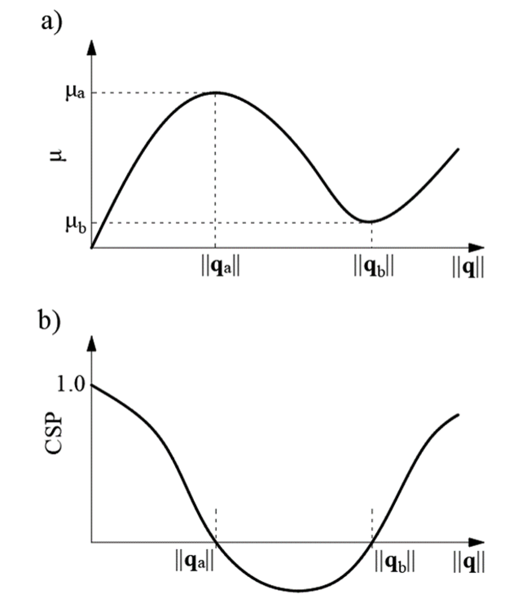
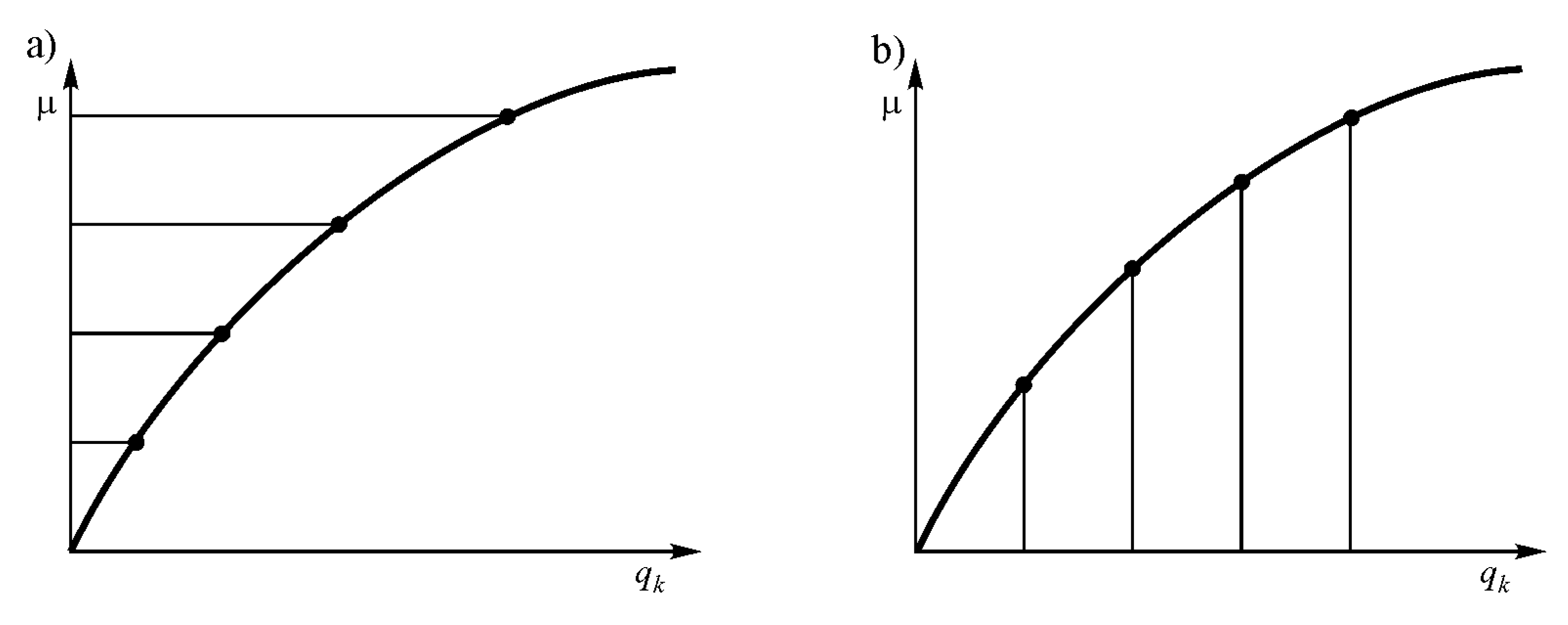
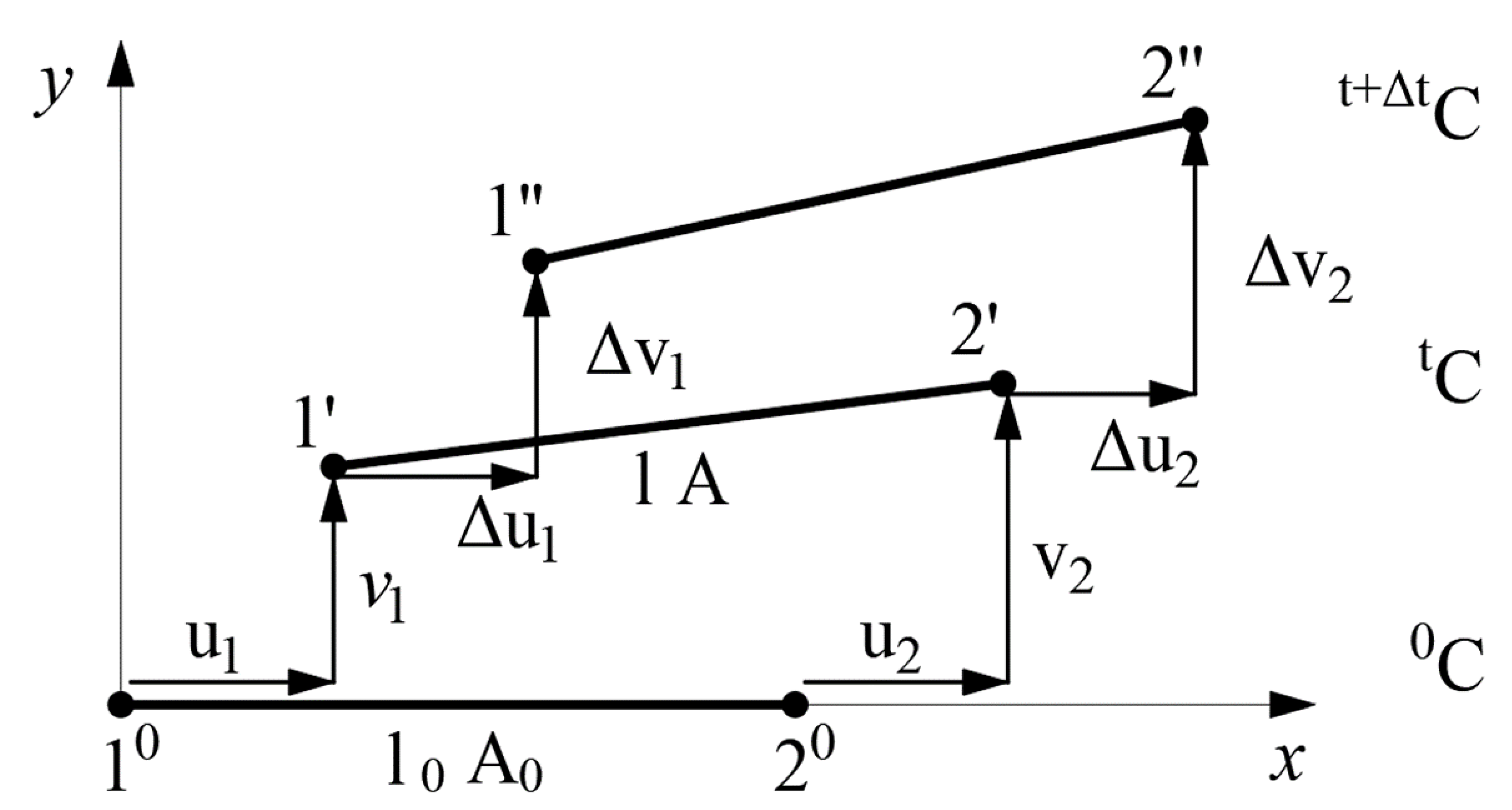
2.1. Truss Element Description
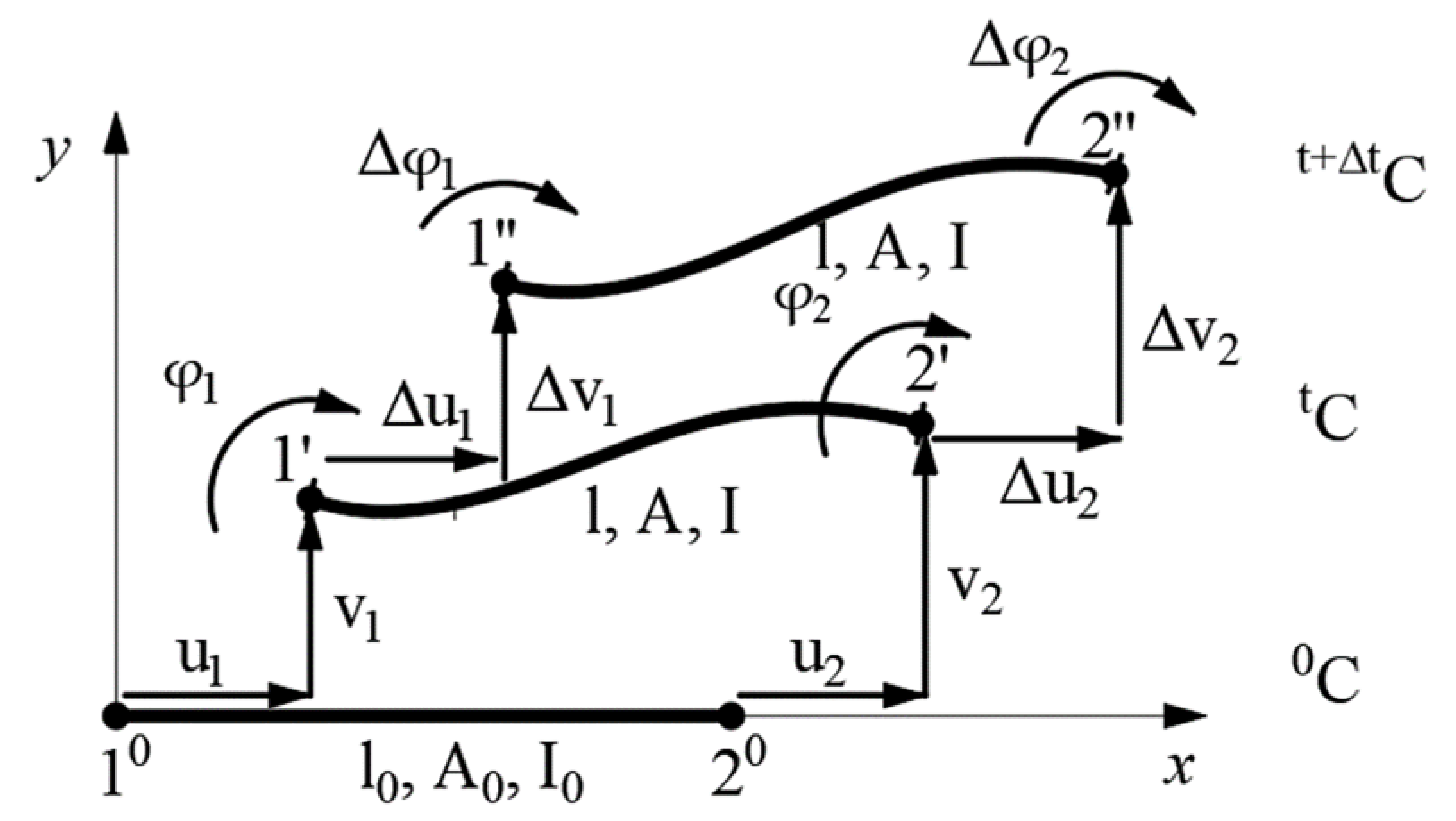
2.2. Frame Element Description
3. Results
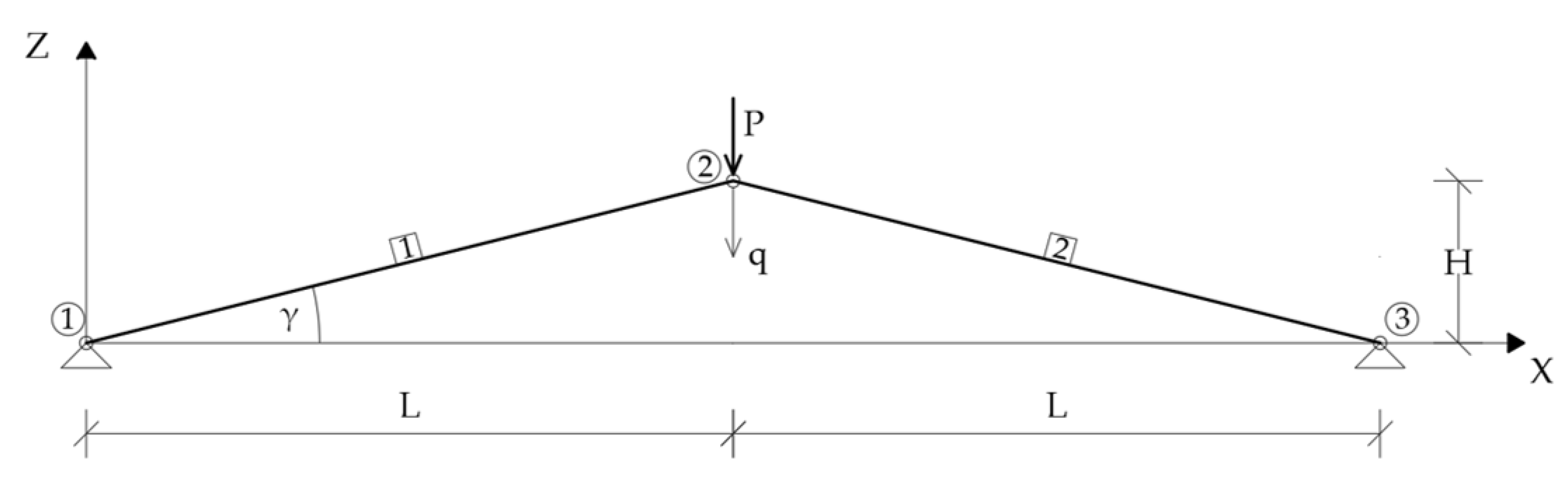
3.1. Example 1
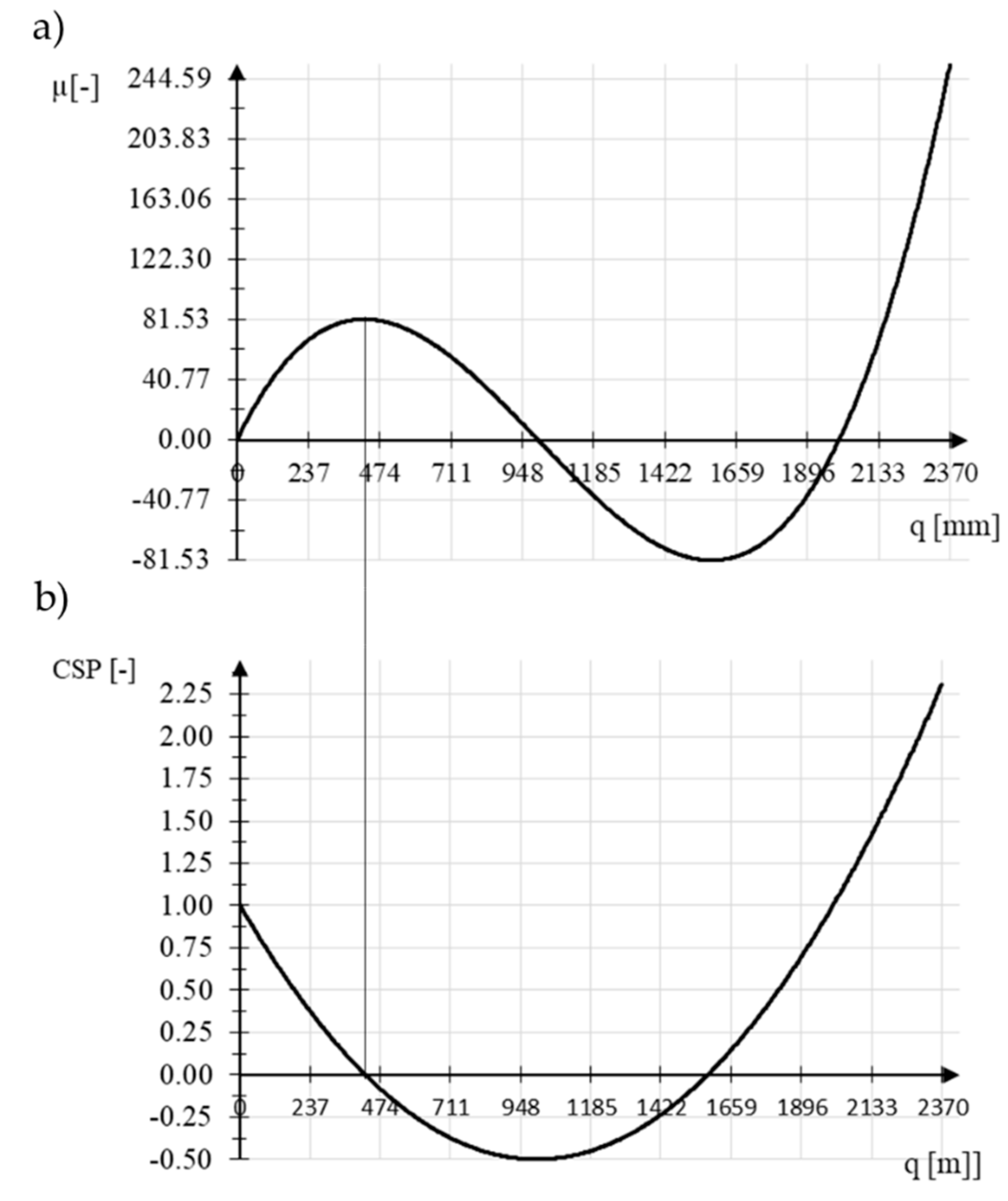
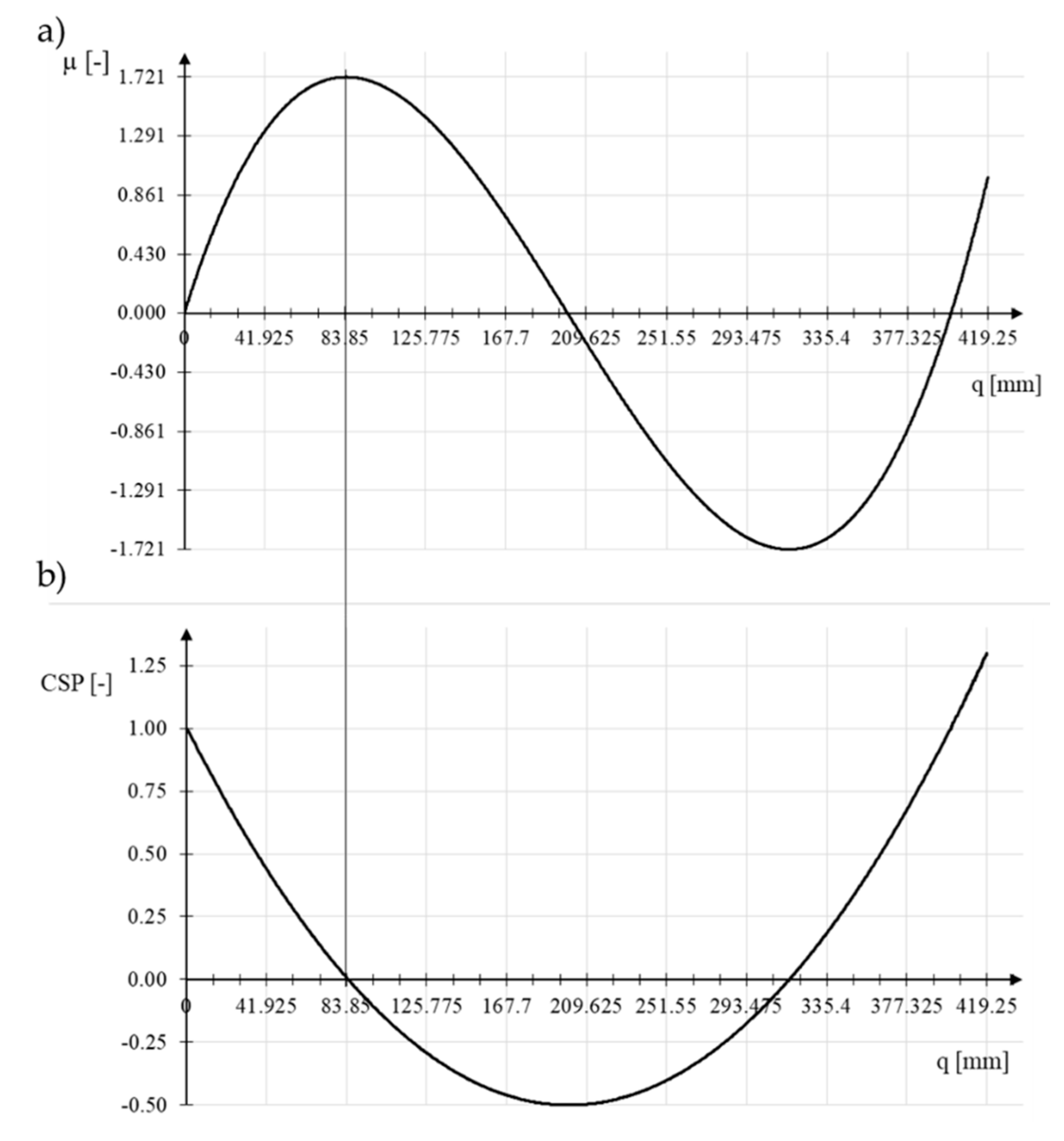
3.1.1. Von Mises Truss Analysis
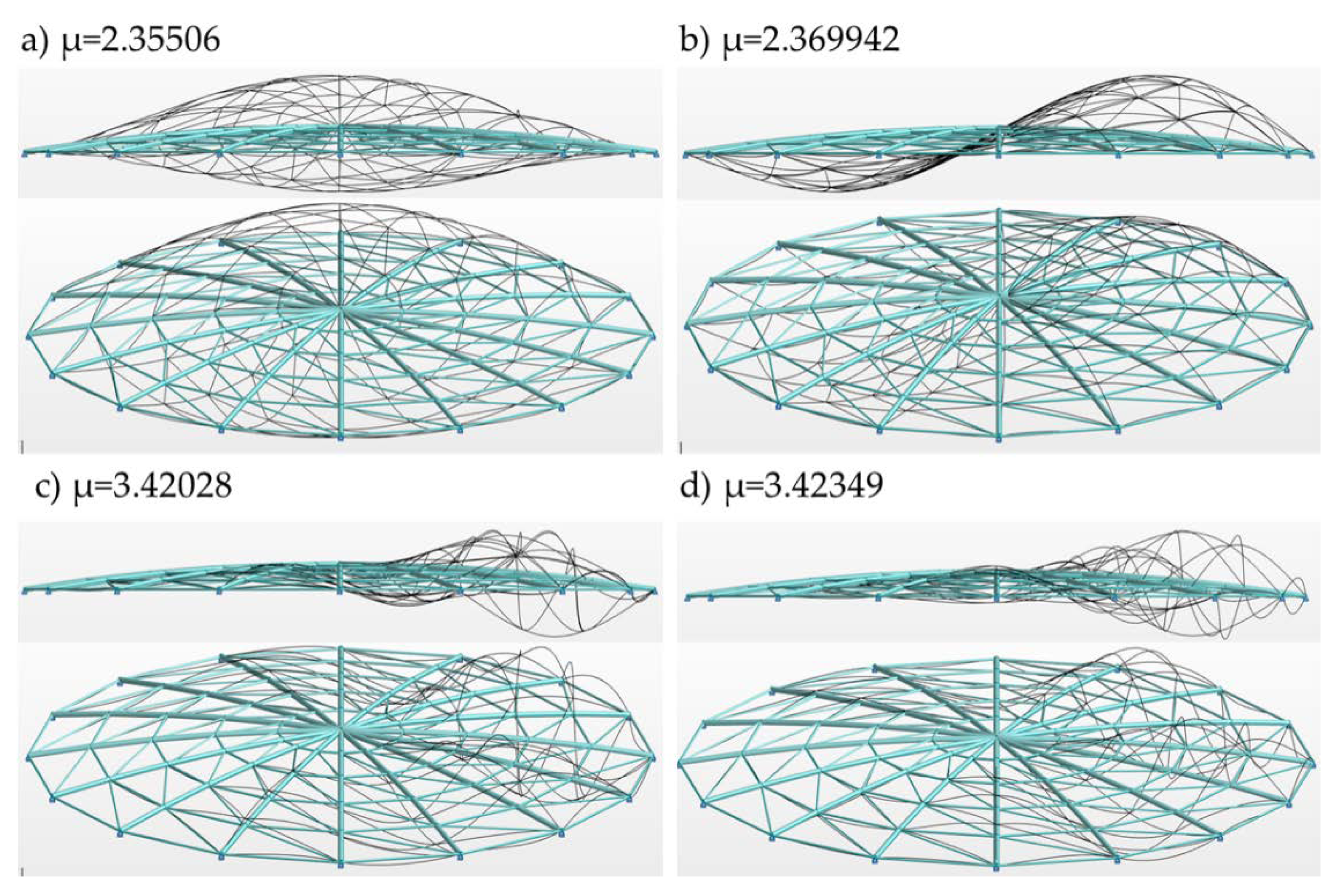
3.1.2. Discussion of Example 1
3.2. Example 2
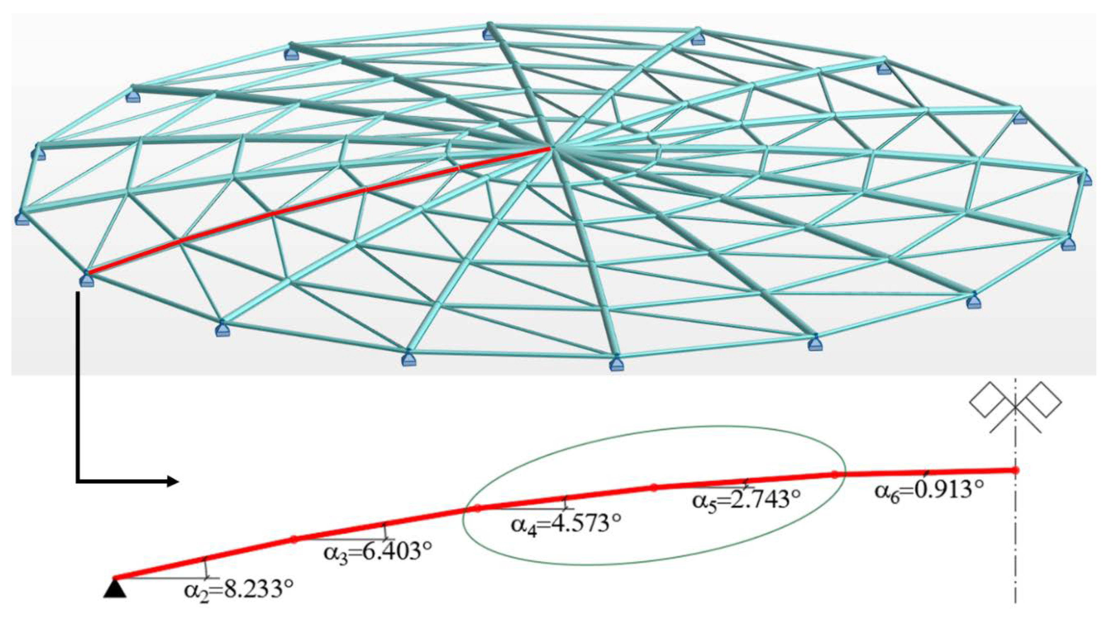
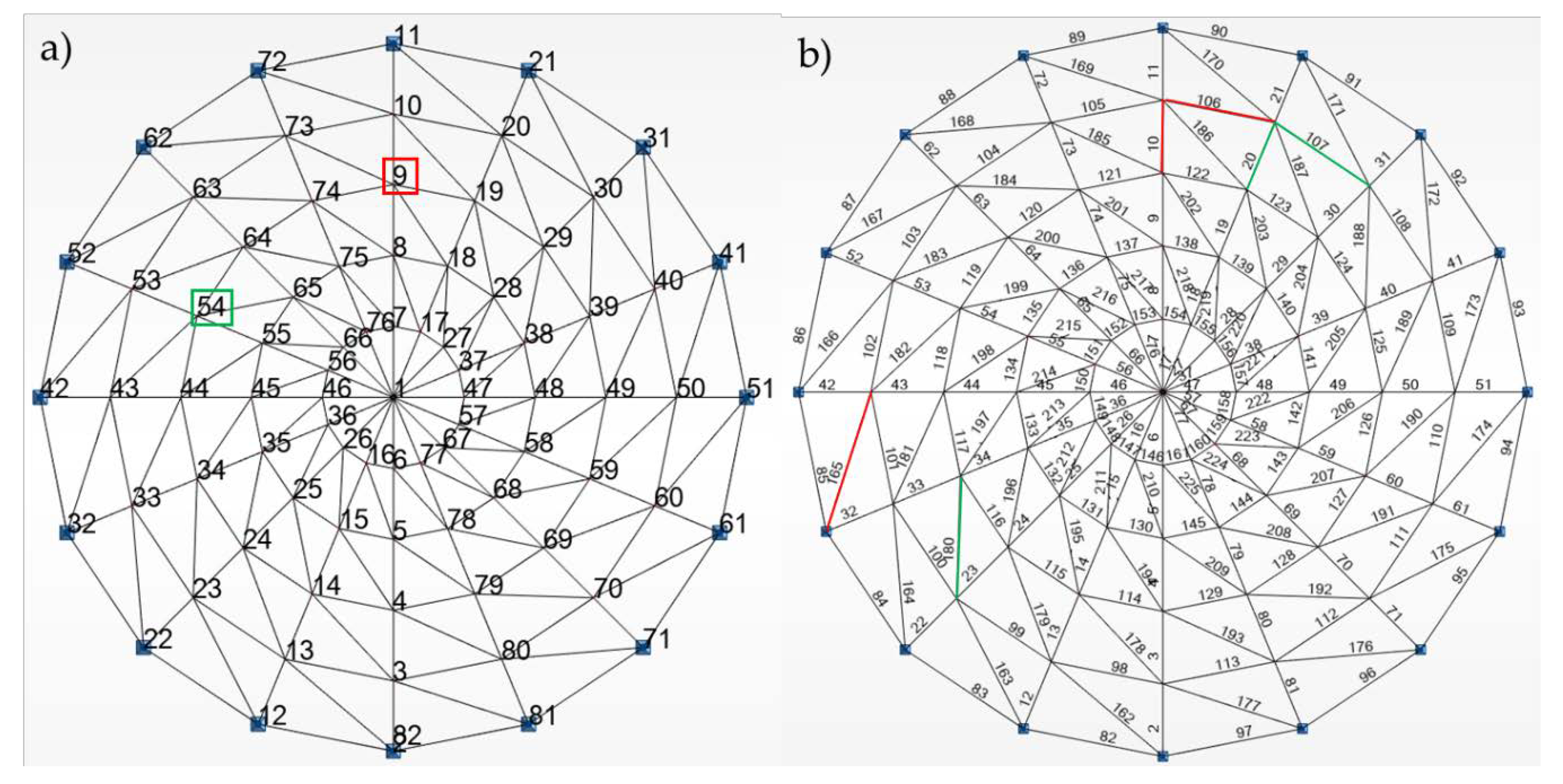
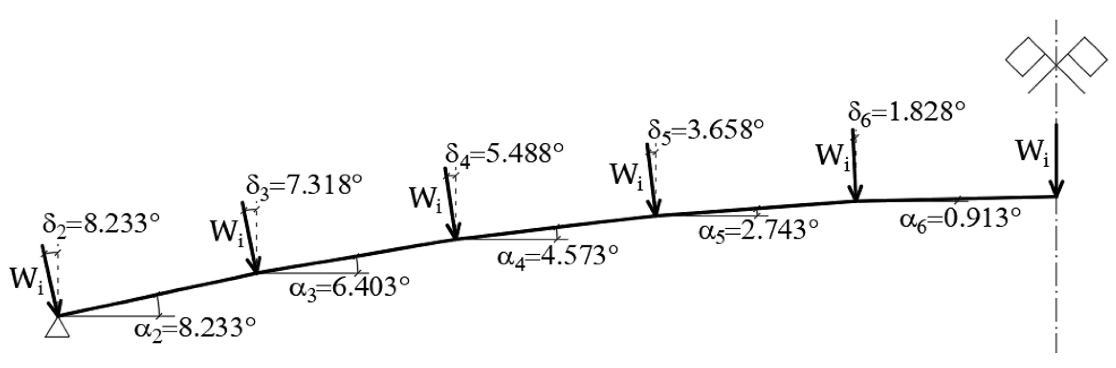
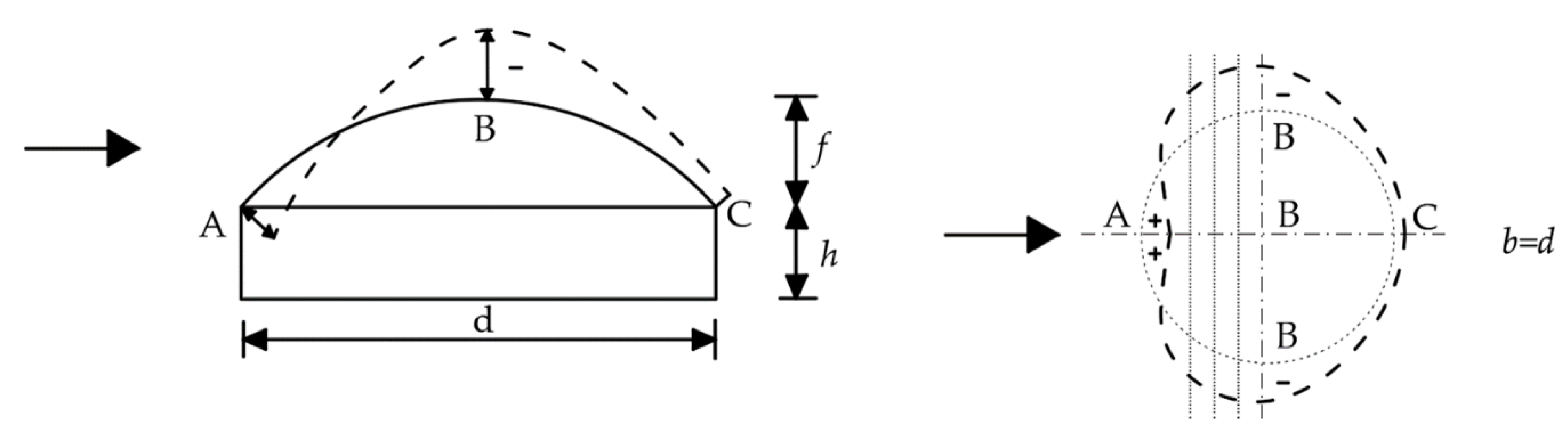
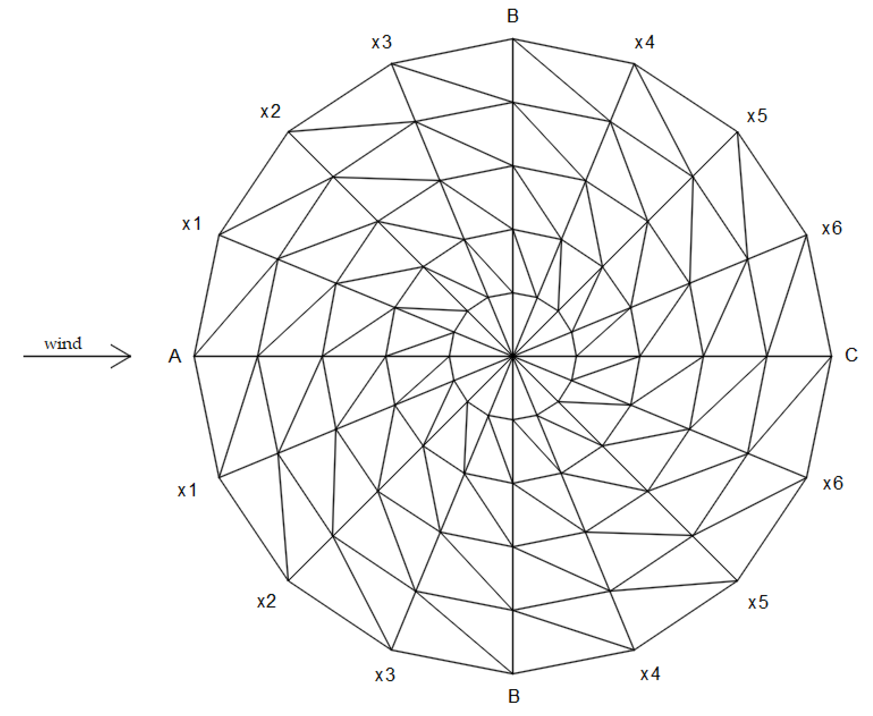
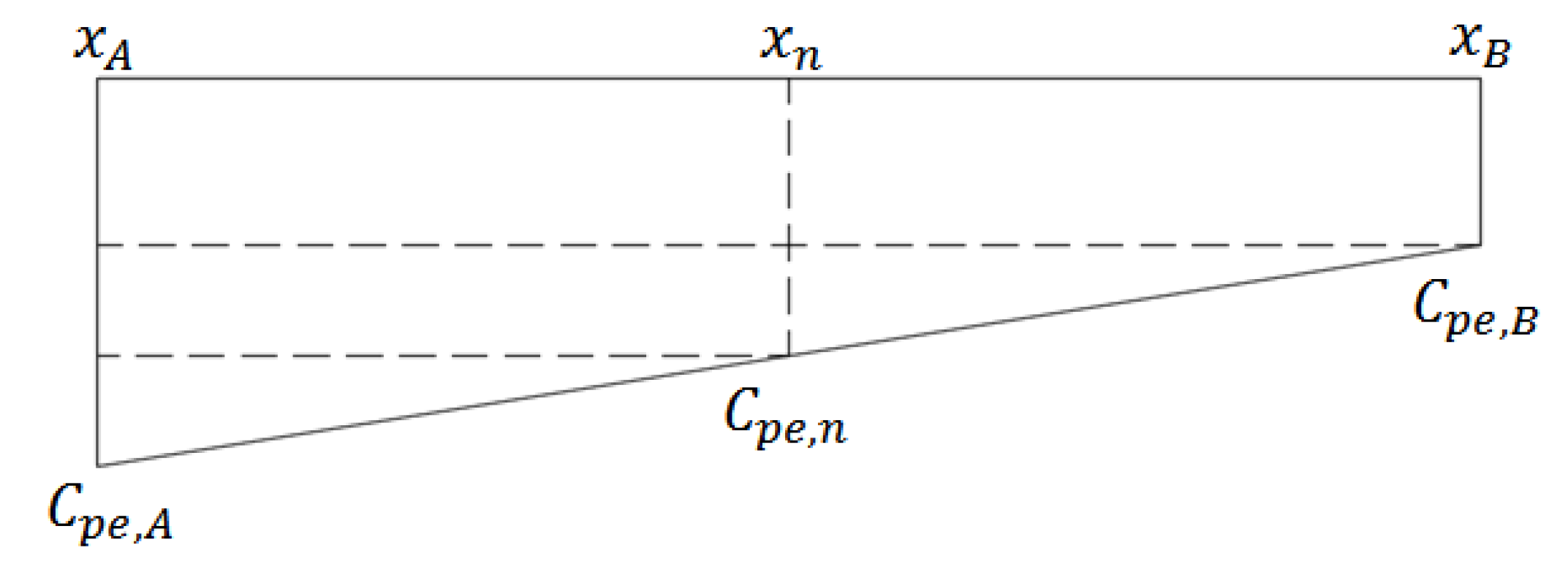
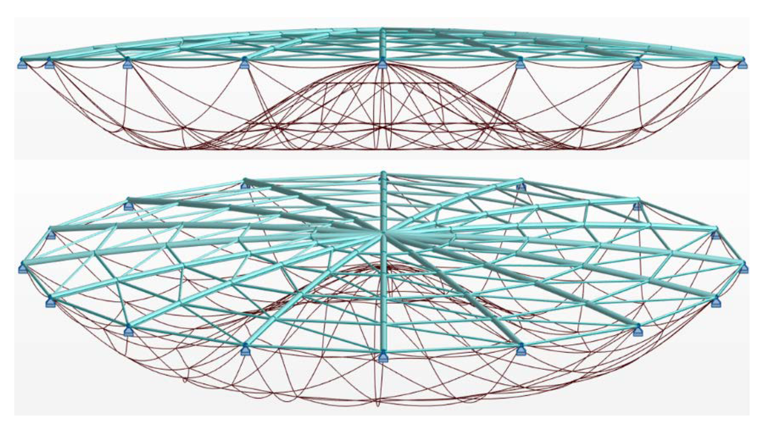
3.2.1. Geometry and Loads
3.2.2. Case 1. Load Combination: 1.15G + 1.5S
3.2.3. Case 2. Load Combination 1.15 × G +1.5 × S+0.9 × W
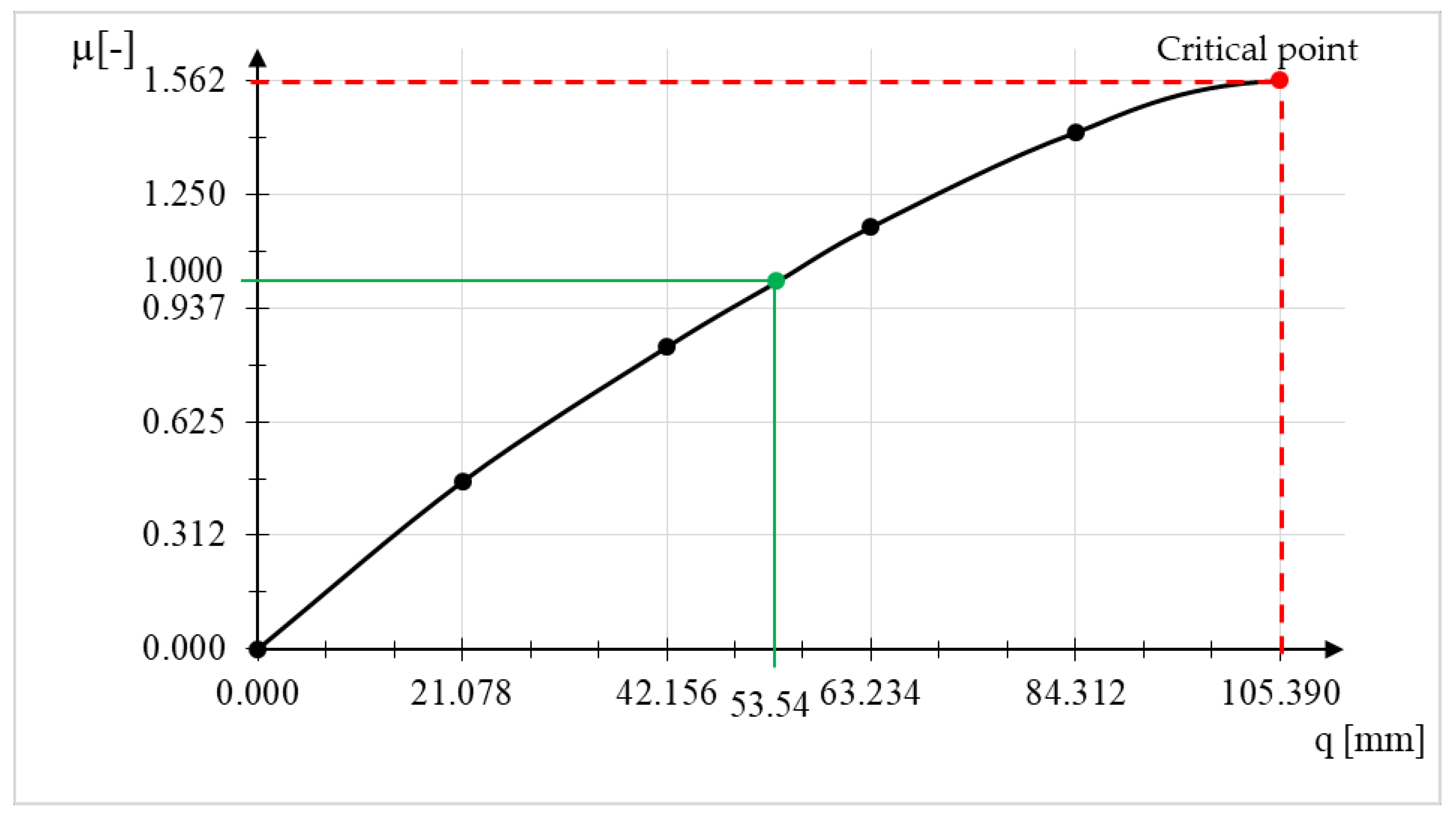
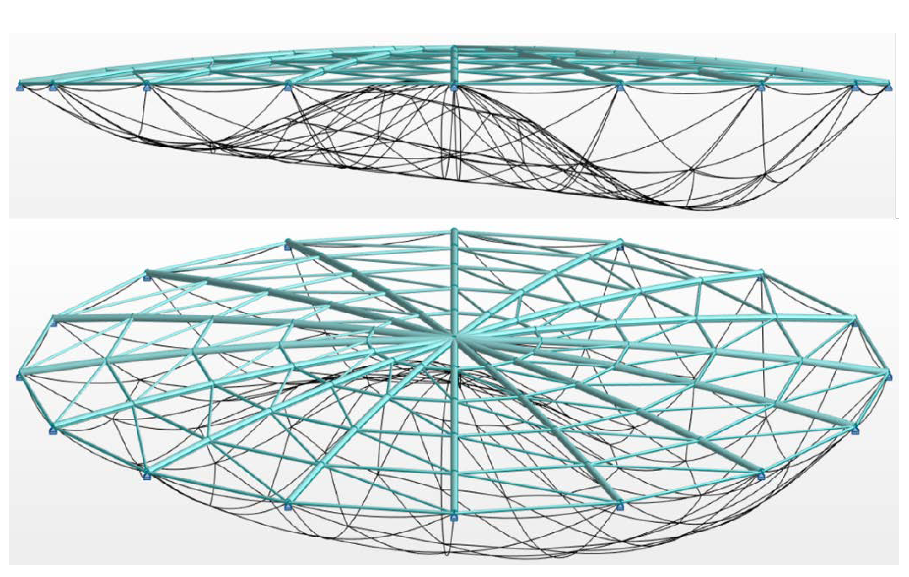
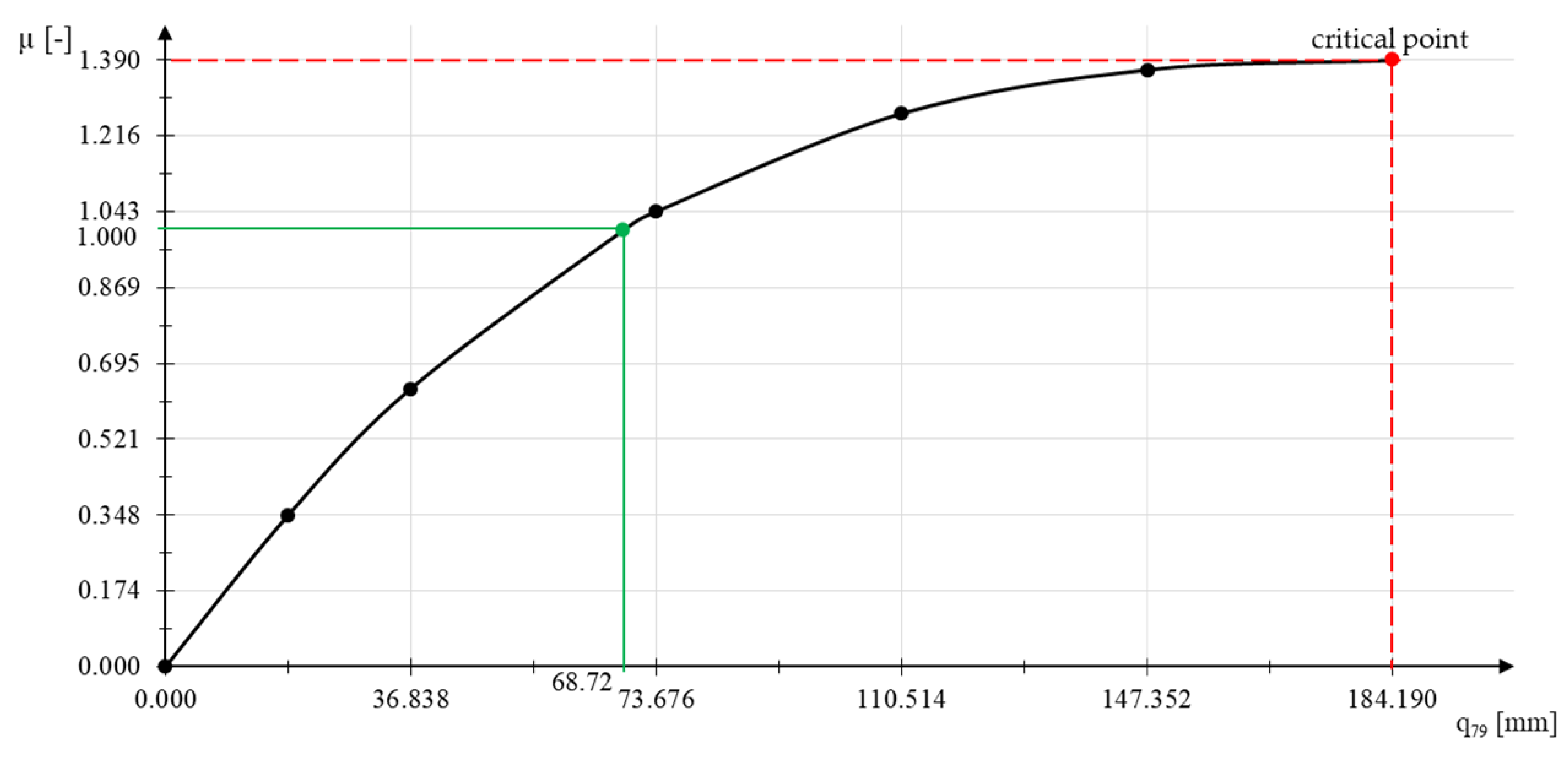
3.2.4. Discussion of Example 2
4. Conclusions
Author Contributions
Funding
Conflicts of Interest
References
- Kozłowski, A. Steel Structures. Examples of Calculations According to PN-EN-1993-1. Part I. Selected Elements and Connections; Oficyna Wydawnicza Politechniki Rzeszowskiej: Rzeszów, Poland, 2009. (In Polish) [Google Scholar]
- Giżejowski, M.; Ziółko, J. General Construction, Steel Constructions of Buildings. Design According to Eurocodes with Examples of Calculations; Arkady: Warsaw, Poland, 2010; Volume 5. (In Polish) [Google Scholar]
- PN-EN 1993-1-1. Eurocode 3: Design of Steel Structures. Part 1–1: General Rules and Rules for Buildings; PKN: Warsaw, Poland, 2005. [Google Scholar]
- Szychowski, A. Stability of cantilever walls of steel thin-walled bars with open cross-section. Thin-Walled Struct. 2015, 94, 348–358. [Google Scholar] [CrossRef]
- Szychowski, A. The stability of eccentrically compressed thin plates with a longitudinal free edge and with stress variation in the longitudinal direction. Thin-Walled Struct. 2008, 46, 494–505. [Google Scholar] [CrossRef]
- Oda, H.; Usami, T. Stability design of steel plane frame by second-order elastic analysis. Eng. Struct. 1997, 19, 617–627. [Google Scholar] [CrossRef]
- Fan, F.; Yan, J.; Cao, Z. Elasto-plastic stability of single-layer reticulated domes with initial curvature of members. Thin-Walled Struct. 2012, 60, 239–246. [Google Scholar] [CrossRef]
- Ramalingam, R.; Jayachandran, S.A. Postbuckling behavior of flexibly connected single layer steel domes. J. Constr. Steel Res. 2015, 114, 136–145. [Google Scholar] [CrossRef]
- Plaut, R.H. Snap-through of shallow reticulated domes under unilateral displacement control. Int. J. Solids Struct. 2018, 148–149, 24–34. [Google Scholar] [CrossRef]
- Xu, Y.; Han, Q.H.; Parke, G.A.R.; Liu, Y.M. Experimental Study and Numerical Simulation of the Progressive Collapse Resistance of Single-Layer Latticed Domes. J. Struct. Eng. 2017, 143. [Google Scholar] [CrossRef]
- Yan, S.; Zhao, X.; Rasmussen, K.J.R.; Zhang, H. Identification of critical members for progressive collapse analysis of singlelayer latticed domes. Eng. Struct. 2019, 188, 111–120. [Google Scholar] [CrossRef]
- Walport, F.; Gardner, L.; Real, E.; Arrayago, I.; Nethercot, D.A. Effects of material nonlinearity on the global analysis and stability of stainless steel frames. J. Constr. Steel Res. 2019, 152, 173–182. [Google Scholar] [CrossRef]
- Koiter, W.T. On the Stability of Elastic Equilibrium; National Aeronautics and Space Administration: Washington, DC, USA, 1967.
- Oden, J.T.; Fost, R.B. Convergence, accuracy and stability of finite element approximations of a class of non-linear hyperbolic equations. Numer. Methods Eng. 1973. [Google Scholar] [CrossRef]
- Bathe, K.J. Finite Element Procedures in Engineering Analysis; Prentice Hall: New York, NY, USA, 1996. [Google Scholar]
- Belytschko, T.; Liu, W.K.; Moran, B. Nonlinear Finite Elements for Continua and Structures; Wiley: Chichester, UK, 1997. [Google Scholar]
- Kleiber, M. Some results in the numerical analysis of structural instabilities, Part 1 Statics. Eng. Trans. 1982, 30, 327–352. [Google Scholar]
- Biegus, A. Basics of Design and Impact on Building Structures; Oficyna Wydawnicza Politechniki Wrocławskiej: Wrocław, Poland, 2014. (In Polish) [Google Scholar]
- Biegus, A. Builder’s Educational Notebooks. Issue 1. Basics of Structure Design. Actions on Structures. Steel Structure Design; Builder: Warsaw, Poland, 2011. (In Polish) [Google Scholar]
- Bergan, P.G.; Soreide, T.H. Solution of large displacement and stability problem using the current stiffness parameter. In Proceedings of the Finite Elements in Nonlinear Mechanics, Geilo, Norway, September 1977; pp. 647–669. [Google Scholar]
- Riks, E. An incremental approach to the solution of snapping and buckling problems. Int. J. Solids Struct. 1979, 15, 529–551. [Google Scholar] [CrossRef]
- Riks, E. The application of Newton’s method to the problem of elastic stability. J. Appl. Mech. 1972, 39, 1060–1065. [Google Scholar] [CrossRef]
- Crisfield, M.A. A fast incremental/iterative solution procedure that handles snap-through. Comput. Struct. 1981, 13, 55–62. [Google Scholar] [CrossRef]
- Ramm, E. Strategies for Tracing the Non-Linear Response Near Limit Points. Nonlinear Finite Element Analysis in Structural Mechanics; Springer: Berlin/Heidelberg, Germany, 1981; pp. 68–89. [Google Scholar]
- Wempner, G.A. Discrete approximation related to nonlinear theories of solids. Int. J. Solids Struct. 1971, 7, 1581–1599. [Google Scholar] [CrossRef]
- Ritto-Corrêa, M.; Camotim, D. On the arc-length and other quadratic control methods: Established, less known and new implementation procedures. Comput. Struct. 2008, 86, 1353–1368. [Google Scholar] [CrossRef]
- Leon, S.E.; Paulino, G.H.; Pereira, A.; Menezes, I.F.M.; Lages, E.N. A Unified Library of Nonlinear Solution Schemes. Appl. Mech. Rev. 2011, 64, 040803. [Google Scholar] [CrossRef]
- Rezaiee-Pajand, M.; Naserian, R.; Afsharimoghadam, H. Geometrical nonlinear analysis of structures using residual variables, Mechanics Based. Des. Struct. Mach. 2019, 47, 215–233. [Google Scholar] [CrossRef]
- Waszczyszyn, Z.; Cichoń, C.; Radwańska, M. Stability of Structures by Finite Element Methods; Elsevier: Amsterdam, The Netherlands, 1994. [Google Scholar]
- Pawlak, U.; Szczecina, M. Dynamic eigenvalue of concrete slab road surface. IOP Conf. Ser. Mater. Sci. Eng. 2017, 245, 22057. [Google Scholar] [CrossRef]
- Kłosowska, J.; Obara, P.; Gilewski, W. Self-stress control of real civil engineering tensegrity structures. AIP Conf. Proc. 2018, 1922, 150004. [Google Scholar] [CrossRef]
- Obara, P.; Kłosowska, J.; Gilewski, W. Truth and myth about 2D Tensegrity Trusses. Appl. Sci. 2019, 9, 179. [Google Scholar] [CrossRef]
- Zabojszcza, P.; Radoń, U. The Impact of Node Location Imperfections on the Reliability of Single-Layer Steel Domes. Appl. Sci. 2019, 9, 2742. [Google Scholar] [CrossRef]
- Pecknold, D.A.; Ghaboussi, J.; Healey, T.J. Snap-through and bifurcation in a simple structure. J. Eng. Mech. ASCE 1985, 7, 909–922. [Google Scholar] [CrossRef]
- Ligarò, S.S.; Valvo, P.S. A self-adaptive strategy for uniformly accurate tracing of the equilibrium paths of elastic reticulated structures. Int. J. Num. Methods Eng. 1999, 46, 783–804. [Google Scholar] [CrossRef]
- Ligarò, S.S.; Valvo, P.S. Large displacement analysis of elastic pyramidal trusses. Int. J. Solids Struct. 2006, 43, 4867–4887. [Google Scholar] [CrossRef]
- Rezaiee-Pajand, M.; Rajabzadeh-Safaei, N. Exact post-buckling analysis of planar and space trusses. Eng. Struct. 2020, 223, 111146. [Google Scholar] [CrossRef]
- PN-EN 1991-1-3: Eurocode 1: Actions on Structures—Part 1–3: General Actions—Snow Loads; PKN: Warsaw, Poland, 2005.
- PN-EN 1991-1-4: Eurocode 1: Actions on Structures—Part 1–4: General Actions—Wind Actions; PKN: Warsaw, Poland, 2008.
- PN-EN 1990:2004. Eurocode: Basis of Structural Design; PKN: Warsaw, Poland, 2008.


| Force/Displacement/Analysis | LA | GNA |
|---|---|---|
| Axial force | 20.616 kN | 20.660 kN |
| Nodal displacement of node No. 2 | 0.236 cm | 0.237 cm |
| Force/Displacement/Analysis | LA | GNA |
|---|---|---|
| Axial force | 100.125 kN | 116.6 kN |
| Nodal displacement of node No. 2 | 2.236 cm | 2.795 cm |
| Group Name | Numbers of Nodes |
|---|---|
| R1 | 6, 16, 26, 36, 46, 56, 66, 76, 7, 17, 27, 37, 47, 57, 67, 77 |
| R2 | 5, 15, 25, 35, 45, 55, 65, 75, 8, 18, 28, 38, 48, 58, 68, 78 |
| R3 | 4, 14, 24, 34, 44, 54, 64, 74, 9, 19, 29, 39, 49, 59, 69, 79 |
| R4 | 3, 13, 23, 33, 43, 53, 63, 73, 10, 20, 30, 40, 50, 60, 70, 80 |
| R5 | 2, 12, 22, 32, 42, 52, 62, 72, 11, 21, 31, 41, 51, 61, 71, 81 |
| Nodes Group | Own Weight Load Value—G (kN) |
|---|---|
| R1 | 3.564 |
| R2 | 7.129 |
| R3 | 10.683 |
| R4 | 14.229 |
| R5 | 8.878 |
| Node No. 1 | 7.180 |
| Nodes Group | Snow Load Value—S (kN) |
|---|---|
| R1 | 4.059 |
| R2 | 8.118 |
| R3 | 12.165 |
| R4 | 16.203 |
| R5 | 10.110 |
| Node No. 1 | 8.176 |
| Pressure Coefficients | xA | x1 | x2 | x3 | xB | x4 | x5 | x6 | xC |
|---|---|---|---|---|---|---|---|---|---|
| x | 0.00 | 3.125 | 6.25 | 9.375 | 12.50 | 15.625 | 18.75 | 21.875 | 25.00 |
| Cpe | −1.14 | −1.00 | −0.85 | −0.71 | −0.56 | −0.47 | −0.38 | −0.29 | −0.20 |
| Node Number | Wind Load Value (kN) | Node Number | Wind Load Value (kN) | Node Number | Wind Load Value (kN) | Node Number | Wind Load Value (kN) |
|---|---|---|---|---|---|---|---|
| 1 | −2.588 | 21 | −1.385 | 41 | −2.245 | 61 | −3.391 |
| 2 | −5.445 | 22 | −4.06 | 42 | −2.675 | 62 | −1.815 |
| 3 | −8.726 | 23 | −6.506 | 43 | −4.286 | 63 | −2.909 |
| 4 | −6.551 | 24 | −4.885 | 44 | −3.218 | 64 | −2.184 |
| 5 | −4.372 | 25 | −3.26 | 45 | −2.148 | 65 | −1.457 |
| 6 | −2.186 | 26 | −1.63 | 46 | −1.074 | 66 | −0.729 |
| 7 | −0.383 | 27 | −0.729 | 47 | −1.074 | 67 | −1.63 |
| 8 | −0.767 | 28 | −1.457 | 48 | −2.148 | 68 | −3.26 |
| 9 | −1.149 | 29 | −2.184 | 49 | −3.218 | 69 | −4.885 |
| 10 | −1.5311 | 30 | −2.909 | 50 | −4.286 | 70 | −6.506 |
| 11 | −0.955 | 31 | −1.815 | 51 | −2.675 | 71 | −4.06 |
| 12 | −4.7766 | 32 | −3.391 | 52 | −2.245 | 72 | −1.385 |
| 13 | −7.654 | 33 | −5.434 | 53 | −3.597 | 73 | −2.22 |
| 14 | −5.746 | 34 | −4.08 | 54 | −2.701 | 74 | −1.666 |
| 15 | −3.835 | 35 | −2.723 | 55 | −1.802 | 75 | −1.112 |
| 16 | −1.917 | 36 | −1.361 | 56 | −0.901 | 76 | −0.556 |
| 17 | −0.556 | 37 | −0.901 | 57 | −1.361 | 77 | −1.917 |
| 18 | −1.112 | 38 | −1.802 | 58 | −2.723 | 78 | −3.835 |
| 19 | −1.666 | 39 | −2.701 | 59 | −4.08 | 79 | −5.746 |
| 20 | −2.22 | 40 | −3.597 | 60 | −5.434 | 80 | −7.654 |
| - | 81 | −4.776 | |||||
| Internal Forces/Displacement | LA | ||
|---|---|---|---|
| Meridian Bar no 30 | Parallel Bar no 114 | Diagonal Bar no 193 | |
| NEd (kN)—axial force | 563.694 | 162.79 | 1.977 |
| Nc,Rd (kN)—design capacity of the section under uniform compression | 1543.95 | 552.250 | 212.910 |
| Nb,Rd (kN)—design buckling resistance of the compressed element | 1486.389 | 275.405 | 60.072 |
| My,Ed,Max (kNm)—design bending moment with respect to y-y axis | 28.537 | 0.569 | 0.316 |
| My,c,Rd (kNm)—design bending resistance with respect to y-y axis | 102.827 | 16.511 | 4.892 |
| Mz,Ed,max (kNm)—design bending moment with respect to z-z axis | −2.300 | 0.572 | −0.090 |
| Mz,c,Rd (kNm)—design bending resistance with respect to z-z axis | 102.827 | 16.511 | 4.892 |
| Utilization (%) | 67 | 65 | 8 |
| Maximum vertical displacement (mm)—for node 79 | 42.52 | ||
| Allowable vertical displacement (mm)—D/300 | 83.33 | ||
| Maximum horizontal displacement (mm)—for node 79 | 3.93 | ||
| Allowable horizontal displacement (mm)—H/150 | 6.67 | ||
| Group Name | Nodes Nos | Cross Section |
|---|---|---|
| Parallel | 2 to 81 | RO 219.1 × 10 |
| Meridian | 82 to 161 | RO 101.6 × 8 |
| Diagonal | 162 to 224 | RO 76.1 × 4 |
| Internal Forces/Displacement | GNA | ||
|---|---|---|---|
| Meridian Bar no 20 | Parallel Bar no 107 | Diagonal Bar no 180 | |
| NEd (kN)—axial force | 596.243 | 208.020 | 1.61 |
| My,Ed,Max (kNm)—design bending moment with respect to y-y axis | 39.097 | 0.825 | 0.431 |
| Mz,Ed,max (kNm)—design bending moment with respect to z-z axis | −2.774 | −0.628 | −0.119 |
| Utilization (%) | 81 | 85 | 9 |
| Maximum vertical displacement (mm)—for node 54 | 53.54 | ||
| Allowable vertical displacement (mm)—D/300 | 83.33 | ||
| Maximum horizontal displacement (mm)—for node 54 | 5.51 | ||
| Allowable horizontal displacement (mm)—H/150 | 6.67 | ||
| Internal Forces/Displacement | LA | ||
|---|---|---|---|
| Meridian Bar no 10 | Parallel Bar no 106 | Diagonal Bar no 165 | |
| NEd (kN)—axial force | 518.05 | 164.801 | 19.766 |
| Nc,Rd (kN)—design capacity of the section under uniform compression | 1543.95 | 552.25 | 212.910 |
| Nb,Rd (kN)—design buckling resistance of the compressed element | 1486.389 | 275.405 | 43.369 |
| My,Ed,Max (kNm)—design bending moment with respect to y-y axis | 29.862 | 0.693 | 0.122 |
| My,c,Rd (kNm)—design bending resistance with respect to y-y axis | 102.827 | 16.511 | 4.892 |
| Mz,Ed,max (kNm)—design bending moment with respect to z-z axis | −2.235 | −0.617 | −0.019 |
| Mz,c,Rd (kNm)—design bending resistance with respect to z-z axis | 102.827 | 16.511 | 4.892 |
| Utilization (%) | 65 | 67 | 49 |
| Maximum vertical displacement (mm)—for node 9 | 48.42 | ||
| Allowable vertical displacement (mm)—D/300 | 83.33 | ||
| Maximum horizontal displacement (mm)—for node 9 | 4.52 | ||
| Allowable horizontal displacement (mm)—H/150 | 6.67 | ||
| Internal Forces/Displacement | GNA | ||
|---|---|---|---|
| Meridian Bar no 10 | Parallel Bar no 106 | Diagonal Bar no 165 | |
| NEd (kN)—axial force | 555.081 | 214.545 | 36.408 |
| My,Ed,Max (kNm)—design bending moment with respect to y-y axis | 43.965 | 1.210 | 0.173 |
| Mz,Ed,max (kNm)—design bending moment with respect to z-z axis | −2.704 | −0.720 | −0.008 |
| Utilization (%) | 83 | 92 | 90 |
| Maximum vertical displacement (mm)—for node 9 | 68.72 | ||
| Allowable vertical displacement (mm)—D/300 | 83.33 | ||
| Maximum horizontal displacement (mm)—for node 9 | 6.52 | ||
| Allowable horizontal displacement (mm)—H/150 | 6.67 | ||
© 2020 by the authors. Licensee MDPI, Basel, Switzerland. This article is an open access article distributed under the terms and conditions of the Creative Commons Attribution (CC BY) license (http://creativecommons.org/licenses/by/4.0/).
Share and Cite
Opatowicz, D.; Radoń, U.; Zabojszcza, P. Assessment of the Effect of Wind Load on the Load Capacity of a Single-Layer Bar Dome. Buildings 2020, 10, 179. https://doi.org/10.3390/buildings10100179
Opatowicz D, Radoń U, Zabojszcza P. Assessment of the Effect of Wind Load on the Load Capacity of a Single-Layer Bar Dome. Buildings. 2020; 10(10):179. https://doi.org/10.3390/buildings10100179
Chicago/Turabian StyleOpatowicz, Dominika, Urszula Radoń, and Paweł Zabojszcza. 2020. "Assessment of the Effect of Wind Load on the Load Capacity of a Single-Layer Bar Dome" Buildings 10, no. 10: 179. https://doi.org/10.3390/buildings10100179
APA StyleOpatowicz, D., Radoń, U., & Zabojszcza, P. (2020). Assessment of the Effect of Wind Load on the Load Capacity of a Single-Layer Bar Dome. Buildings, 10(10), 179. https://doi.org/10.3390/buildings10100179