Accounting for the Spatial Variability of Seismic Motion in the Pushover Analysis of Regular and Irregular RC Buildings in the New Italian Building Code

Abstract

Pushover analysis is the main methodology adopted in practice-oriented applications for investigating the non-linear response of reinforced concrete (RC) buildings; it is applicable for both new and existing buildings. It is well-known that several limitations characterize this methodology and the scientific literature proposes several non-conventional approaches to provide results comparable to those of the more efficient nonlinear dynamic analysis. In most recent seismic guidelines, some improvements have been introduced, in order to overcome the main drawbacks of conventional pushover methods, in view of practice-oriented applications. In particular, new prescriptions are related to the load profiles and the choice of control nodes, aspects that lead to different results in terms of capacity curves and in the safety assessment. Another relevant point is represented by the spatial combination of effects, which suggests the opportunity of executing simultaneous bi-directional pushover analyses. The aim of this paper is to investigate the effects of the new trends followed by some guidelines about pushover analysis, such as the recent 2018 release of the Italian Building Code. In particular, after a general test of the new conventional procedure for the case of RC buildings, a set of case studies has been generated, consisting of three-dimensional RC-archetypes specifically designed and investigated in order to cover the more significant scenarios. The results in terms of global and local performances are processed and critically analyzed, with the aim of appraising the main differences between the traditional and new approaches and identifying the effectiveness and of the actual improvements achieved.

1. Introduction

The study of the seismic performance of reinforced concrete (RC) buildings has attracted increasing interest among researchers and designers, who rely on a strong theoretical background to exploit both design and assessment procedures, as provided by seismic technical codes and scientific literature. In particular, with regard to new RC buildings, the optimal seismic performance at different limits can be achieved through the methodologies of the well-known Performance Based Design. Instead, for existing RC buildings the definition of the seismic performance is an articulated process, because it is strongly connected to several uncertain aspects, such as: the seismic demand, the knowledge of the structural properties (loads, materials and geometry [1,2]), the methods of analysis, the choices in the modelling and numerical assumptions [3,4].

With regard to the methods of analysis, the choice is between linear and nonlinear approaches. Linear methods can be performed either in static form (by considering only the influence of the first fundamental vibration mode per direction) or in dynamic form (combining the effects due to all vibration modes having participation mass greater than 5%, also called Response Spectrum Analysis (RSA)), where the acceleration values are selected from the relevant response spectra. The use of linear analysis is suggested for design procedures (but in some cases also for existing ones), if the main goal is the preliminary evaluation of the stress states in structural elements, for determining the suitability of section dimensions and steel reinforcements.

In order to simulate the real behaviour of existing buildings, the most powerful tool is nonlinear analysis, which investigates the structural response in the post-elastic field, accounting for geometrical and mechanical nonlinearities. To perform nonlinear analysis, it is possible to adopt static or dynamic seismic actions. Generally, the nonlinear dynamic analysis is considered the most effective way to proceed, because it allows accurately simulation of the response of the buildings under seismic motion. On the other hand, despite the availability of a huge variety of scientific works about this topic, in practice-oriented applications nonlinear dynamic analysis has difficulty finding space for several reasons: the design code provisions about the assessment of existing buildings are still lacking; there is an objective difficulty in the selection of ground-motions (number of accelerograms, efficiency, sufficiency [5]); a detailed characterization of the cyclic behaviour of structural elements is needed, high time-analysis and computational efforts are required.

The most valid alternative is represented by the non-linear static analysis, which finds a wide application among designers for its simplicity and analogy with linear analysis. Design codes often have a much more comprehensive and accessible approach to nonlinear static analysis, both for new and existing RC buildings, making it a natural choice for professionals. Furthermore, the recent release of new technical standards, such as the new Italian Building Code (NTC18) [6], has introduced additional references that have in fact widened the scope of applicability of non-linear static analysis.

The presented study aims to explore the spatial variability of the seismic motion by employing the method of nonlinear static analysis, prior to exclusively adopting nonlinear dynamic analysis. In this regard, it is worth remembering that NTC18, following the Eurocode 8 provisions [7], allows performing nonlinear dynamic analysis, by considering some groups of accelerograms, for which each group is made up of three components, such as two horizontal and one vertical component. The starting point is the attempt that the recent updates of Italian guidelines proposed, in which some new indications have been added about the execution of nonlinear static analysis; that will be analysed in the paper. Of course, the interpretation provided is only intended to be a critical discussion by the authors of the additional requirements presented in the new technical code. Operationally, the study presents a sensitivity analysis on a set of case studies properly defined, with the objective to critically evaluate the effects on the global performance of the buildings and on the local performance of the structural elements. It was decided to refer to a very simple archetype-RC building which has been progressively modified, in order to represent different levels of in-plane irregularity. A large set of numerical models were analysed and investigated, as presented in the following sections, and the results provide interesting suggestions about the performance of alternative conventional pushover analyses, highlighting when they can improve the performance evaluation.

2. Pushover Analysis: Brief Overview about Conventional and Non-Conventional Methods

The study of the seismic performance of RC buildings through nonlinear static analysis consists of the application of a static load pattern distributed along the height of the building, which is monotonically increased step-by-step until the global collapse mechanism of the structure is reached. The structural response is expressed through the capacity curve, which is a scalar force–displacement relationship usually recorded in terms of base shear (V_b) vs. roof displacement (δ_R), monitored on a control node (CN). To define the safety level of the building under investigation, the capacity curve is compared with the seismic demand according to established approaches, such as the N2 method [8] as applied in [9], without forgetting the absolute validity of the capacity spectrum method, as implemented in [10] and in [11] for irregular buildings.

The results of the analysis are strongly dependent on the shape of the load pattern adopted, which can be generally written as, Equation (1):

$$\overline{F}=\overline{\Psi }·\lambda \left(t\right)$$

(1)

where F is the force vector of the load profile, Ψ is a time-independent shape vector defining the distribution of the inertial forces along the height and λ is the factor that defines the amplitude of the inertial forces as a function of the analysis step (t). Some technical standards, such as the Italian NTC18, recommend performing pushover analysis by using at least 2 different load profiles that could represent the inertial force distribution induced by earthquakes. In particular, a pair of possible load distributions is represented by the uniform load profile, proportional to the building masses (Equation (2)), and the inverse triangular load profile, proportional to the building height.

The latter could be substituted by the “unimodal” load pattern, dependent on the eigenvector related to the first fundamental vibration mode of the building along the considered direction (Equation (3)). The two above-mentioned load patterns can be written as follows in Equations (2) and (3):

$$\overline{F}=\left[M\right]·\overline{I}·\lambda \left(t\right)$$

(2)

$$\overline{F}=\left[M\right]·\overline{{\Phi }_1}·\lambda \left(t\right)$$

(3)

where [M] is the mass matrix, $\overline{I}$ is the identity vector and $\overline{{\Phi }_1}$ is the eigenvector of the first modal shape.

The reasons for this requirement are related to the necessity of combining the advantages of the unimodal profiles, which are able to predict the behaviour in the elastic field, and the uniform profiles, which are suggested in case of strong plastic deformations, especially at lower storeys. The adoptions of these load profiles is allowed only with a participating mass (M[%]) greater than 75% in the direction of the analysis.

This conventional procedure of the pushover analysis is characterized by two main limitations: (a) the use of the unimodal load profile does not consider the influence of higher modes, which might be significant in specific situations; and (b) the assumption of time-invariant load profiles does not account for the progressive stiffness variation of the structural elements, and therefore neglects the variation of the structural dynamic properties (periods, fundamental modes shape).

To overcome these drawbacks, several alternative, non-conventional methodologies have been developed, which can be classified in 2 macro-groups: (i) multimodal pushover; and (ii) adaptive pushover.

The multimodal pushover analysis is a tool that allows taking into account the influence of higher modes, especially for buildings presenting a high number of floors (the first periods are high and fall into the right part of the response spectrum) or structural irregularities (in mass or stiffness). The above-mentioned topics have attracted large interest among researchers, who have developed several proposals of multimodal pushover analysis to take into account the torsional behaviour of RC buildings [12,13]. Considering the nonlinearity of the problem, the scientific literature proposes two main approaches: (a) a combination of the significant modes into a unique load profile, before performing the analysis; or (b) a combination of the effects after performing a set of unimodal pushover analyses proportional to the modes to be considered.

In the first category, in [14] the authors have investigated a case study through the method of modal combination (MMC), firstly by applying a sum and a difference of the first two vibration modes and after by defining new participation factors dependent from the seismic demand and the elastic period of the considered modes. A similar approach is presented in [15], where a participation factor α to be employed in modal combination is proposed. The authors assessed the reliability of the proposal on 3D archetype-RC buildings having different features (regular, irregular in stiffness, irregular in mass) and they compared the results with nonlinear dynamic analyses. A more recent research is [16], in which the authors proposed a generalized pushover analysis (GPA) conceived for taking into account the force distribution in 3D torsionally coupled systems based on the maximum interstorey drift obtained under seismic action. In [17], a unique load profile was proposed, through the modal decomposition of the maximum displacements vector ($\overline{u_{max}}$) obtained by the complete quadratic combination (CQC) of the linear effects after response spectrum analysis. In particular, the contributions of all modes considered were weighted through the definition of new participation factors z_n, Equation (4):

$$z_n=\frac{{\overline{{\Phi }_n}}^T·\left[M\right]}{{\overline{{\Phi }_n}}^T·\left[M\right]·\overline{{\Phi }_n}}·\overline{u_{max}}$$

(4)

where n indicates the used vibration modes. Other works worth mentioning are [18,19,20,21,22,23,24].

In the second category, a key role is played by the works of Chopra and Goel [25], who were the first to propose the modal pushover analysis (MPA). The method consists in performing several unimodal pushover analyses proportional to the first and to the higher modes, and then combining the effects through CQC or square root of sum of square (SRSS). The authors themselves observed that the main problem was the poor prediction of the post-elastic behaviour, because the above-mentioned combination rules are theoretically valid in the elastic field. In the following works, the authors improved the procedure [26,27,28], making some modifications to the effects of the combination rules and by investigating a large sample of tall and irregular buildings.

With regard to the adaptive pushover, some authors have proposed methods for accounting for time-variant load profiles. The first versions can be found in [29,30,31]. Based on the achievements of the previous methods, in [32] the authors proposed an algorithm named Force Adaptive Pushover (FAP), which consists of computing the stiffness modification at some steps of the analysis (identified through the achievement of pre-defined interstorey drift values) and accordingly re-computing the load profile. The method was tested on some stick-models, opportunely defined to represent a large casuistry of buildings. In [33] the same authors developed a similar procedure, named displacement adaptive pushover (DAP), which consists of the application of a displacement profile in the analysis. The results showed an improvement in the prediction of the structural behaviour (compared with the results of nonlinear dynamic analyses), but the method retains the well-known limitation of the used combination rules (CQC and SRSS) in the post-elastic field. Other methodologies were recently proposed and are worth mentioning [34,35,36].

Both conventional and non-conventional approaches to pushover analysis describe the evolution of the structural capacity in the post-elastic field but, in many cases, do not take into account the spatial effects of the ground excitation, which are instead captured by employing nonlinear dynamic analysis. In addition, it is worth remembering that the nature of pushover analysis is to investigate the building performance along a single direction and to use static forces, neglecting the multi-directional effect of the seismic motion, as investigated in [37]. By following this framework, some research works can be mentioned which have the possibility to account for the spatial effects of the seismic motion by matching the easiness of pushover analysis and the good prediction skills of nonlinear dynamic analysis, and then the implementation of bi-directional pushover analysis (considering or not conventional and non-conventional load patterns).

In [38] the authors proposed the bidirectional pushover analysis (BPA), a consistent method with the N2 proposed for irregular in-plan buildings [39] and in-height buildings [40]. In particular, the method consisted in the application of two simultaneous unimodal load profiles in both main directions of 3D structures. The capacity curve was recorded in only one direction and, through the N2 method, the seismic performance was computed accounting for the influence of the other main direction, which is intrinsically contained in the capacity curve. Other kinds of bi-directional pushover analyses can be mentioned, which also considered the multimodal combination of the load profiles [41,42,43].

3. New Provisions about Conventional Pushover Analyses in the Italian Building Code

The recent release of the NTC 2018, in agreement with Eurocode 8 [7], has introduced some additional indications about pushover analysis:

• It is necessary to consider alternative control nodes, such as the corner points of the last storey, especially when the structural system presents a significant coupling among translations and rotations;
• It is possible to use a load profile proportional to the distribution of the storey shears as computed by an elastic response spectrum analysis (RSA). This load pattern can be used in any case; it can also be used if the participating mass M[%] in the direction considered is lower than 75%. Furthermore, the use of this profile is mandatory if the fundamental period of the structure is greater than 1.3 times the corner period (T_c);
• The effects of seismic motion in the 3 directions must be combined according to the same formula already present for RSA, which takes into account the 3 spatial components of an earthquake. In particular, the principal component is considered with a unitary coefficient, while the others are reduced to 30%. The analysis must be repeated by alternating the reduction coefficients among the components. Assuming that the direction X is the principal direction, the combination rule is written as follows, according to Equation (5):

  $$E_X+0.3E_Y+0.3E_Z$$

  (5)

  where E_X, E_Y and E_Z (usually neglected for typical building structures) are, respectively, the responses in the two main horizontal directions and the vertical direction of the building. The safety assessment shall consider the heaviest effects obtained.

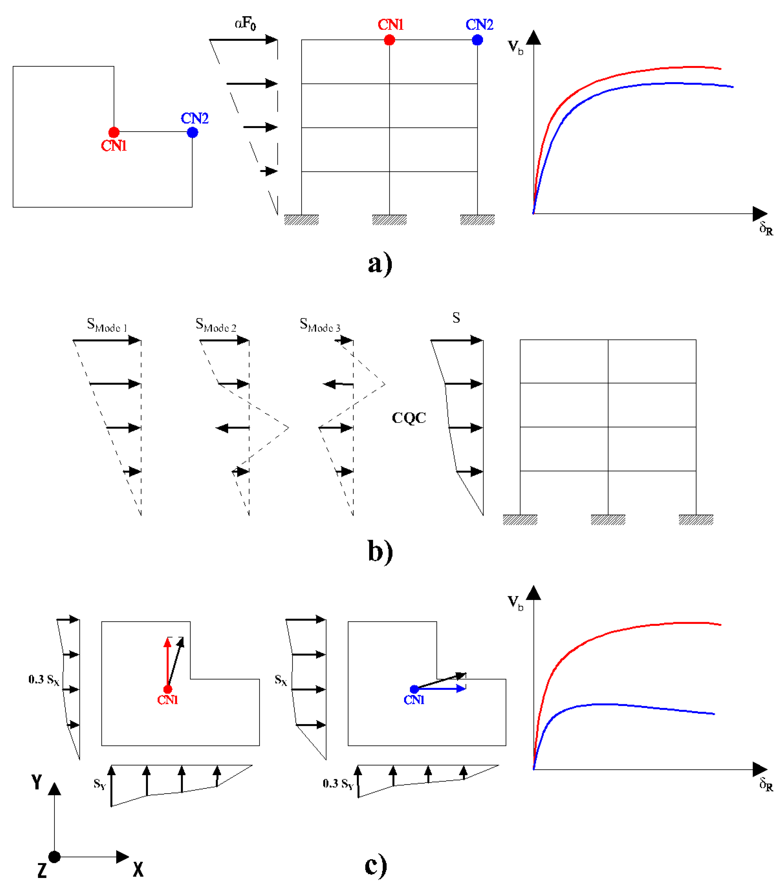
Considering that these provisions, depicted respectively in Figure 1a–c, open new perspectives about the conventional pushover analysis, it is worth discussing each of them in order to investigate the actual improvements that the new rules can bring to the seismic performance assessment.

With regard to the first point, the choice of different positions of the control node (CN) for monitoring the capacity curve was studied by the authors of this paper in a previous work [44], in which several regular existing RC buildings, with different configurations in plan and a number of floors, were analysed, and the position of the control node CN was varied within the last storey.

It is important to highlight two different key aspects: (i) the monitoring of different CNs results in capacity curves having a different shape, which does not mean that the building behaviour changes; and (ii) the CN should represent a point where the mass of the entire storey can be condensed to effectively simulate an equivalent dynamic response, in analogy with a “lollipop” multi degree of freedom (MDOF) system, whereas the assumption of a corner CN does not reflect a real physical mass distribution in the building. On the other hand, especially for irregular in-plan buildings, the use of different CNs could be a conservative choice, because it provides different configurations of the global capacity, different inputs for the N2 method performance and different values of the safety level, here expressed as the demand/capacity ratio (D/C).

The second provision establishes the possibility to always perform a pushover analysis, even when the participating mass M[%] in the direction investigated is lower than 75%. Based on the issues mentioned in Section 2, for which the scientific community has long investigated alternative non-conventional approaches, this represents a strong assumption. According to the NTC2018 suggestion, in order to define this load profile it is first necessary to perform an elastic RSA on the building, by using the demand response spectrum at the relevant limit state and then evaluate the storey shears at each floor and normalize them into a unique load profile. In further detail, the shear response in each direction represents the maximum probable seismic response obtained from the contribution of all the vibration modes having a M[%] greater than 5%, for a total M[%] not lower than 85%, combined through a CQC. The improvements obtained by the use of this load profile are a first object of investigation in this paper, with the aim of evaluating the differences compared to other conventional load profiles.

The third provision adds a rule for considering the effects of the spatial variability of the motion by using a “nonlinear” version of the combination of effects used for RSA (Equation (5)). This concept deserves some discussion. When applying Equation (5) to the RSA, which is a linear problem, the term “E” represents the response of the seismic analysis and it is always proportional to the actions. The extension of the same rule to a non-linear problem, however, is questionable. Combining the effects derived from separate pushover analyses performed along different directions at a final performance point is in contrast with the basic concepts of the method itself, which is an incremental approach, non-dependent on the initial module of the loads, but only from the shape; such an effect-combination will never provide the same response as given by an actual combination of the input. The indication of the code could be interpreted differently, as a combination of forces, by applying a load profile that is unitary in the monitored main direction and reduced by a 0.30 scale factor in the other main directions. Based on these considerations, this aspect is investigated in this paper by performing pushover analyses with a “combined” load profile and critically comparing the results with the standard procedure (as provided by the previous codes).

4. Application of Directional Pushover on 3D RC Archetypes: General Information

The investigation was performed on a sample of 8 RC low-rise archetype buildings, all designed for the same level of seismic action and all presenting different modal properties. In particular, they present a regular in-plan configuration and, according to the reference system in Figure 2, the participating mass in the Y direction is gradually changed while the one in the X direction is kept unchanged.

The reference model (B_REG) is extremely regular in both main directions (M[%] > 85%). Starting from this model, the other ones were derived by varying some of the structural elements in order to obtain a variation in the M[%] in the Y direction from 75% to 45%, with a progressive step of 5% (the models have been labeled as B₇₅, B₇₀, B₆₅, B₆₀, B₅₅, B₅₀, B₄₅). More details about the numerical models are given in Section 4.1.

For each numerical model, several pushover analyses were performed in the two main horizontal directions (the subscripts X and Y indicate the direction of the analysis), adopting different load profiles: unimodal (F); inverse triangular (T); uniform (U); proportional to the building masses (M); and proportional to the storey shears (S). Furthermore, using the S load profiles, two bi-directional pushover analyses were performed, the first monitoring the X direction and using the following force combination (S_X+03Y), as shown in Equation (6):

$$S_X+0.3S_Y$$

(6)

and the second one monitoring the Y direction under the following combination of force profiles (S_Y+03X), Equation (7):

$$0.3S_X+S_Y$$

(7)

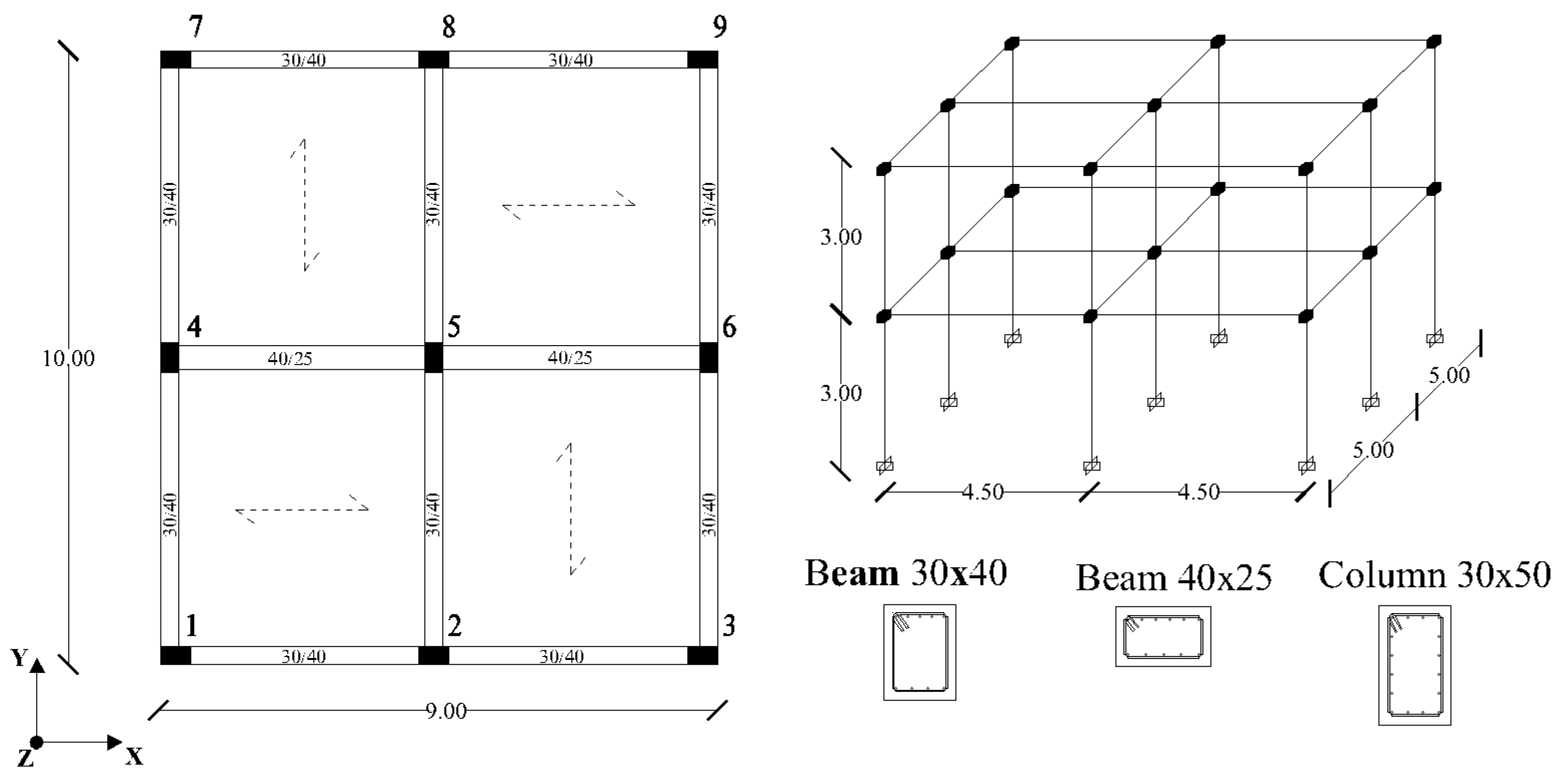
The vertical component was neglected. No eccentricities and inversions in the analysis direction were considered. For each model and analysis, 3 control nodes (CNs) were monitored on the last story: nodes 5, 7 and 9 (see Figure 2). For assessing the global capacity, all the pushover curves were recorded whereas, for the assessment of the local capacity, the response of the base columns under the nodes 5, 6, 7 and 9 (Figure 2), were controlled.

4.1. Description of the Case Studies and Numerical Modelling

The reference model B_REG is a RC building designed according to NTC2018 in “Low” ductility class. From a geometrical point of view, it has a regular shape in-plan, with dimensions 9.00 m in the X direction and 10.00 m in the Y direction, 2 equal bays in both main directions and 2 floors with an inter-storey height of 3.00 m, as shown in Figure 2. No staircases are considered, and floor slabs are disposed as a checkboard. The materials considered are a class C28/35 concrete (cylindrical compressive strength of 28 N/mm²) and a class B450C steel for reinforcements (tensile yielding stress of 450 N/mm²). Vertical service loads are evaluated in the case of residential use. Concerning the seismic action, the response spectrum has been computed for the municipality of Bisceglie (latitude = 16.5052°, longitude = 41.243°), Puglia Region, Southern Italy, which is a low-medium seismicity site. According to a probability of exceedance of 10% in 50 years and an A soil category, for a nominal life of 50 years and a second usage class, the spectral parameters are: a_g = 0.134g, F₀ = 2.495; and T_c^* = 0.377s (according to NTC18 or Eurocode 8 symbology; where g is the constant of gravity acceleration). The vertical component of the seismic action has been neglected, while a behaviour factor q of 3.9 is accounted.

After performing an RSA through the role of Equation (5), the maximum stress states were used for design of the elements section and the result is shown in Figure 2. In particular, side beams have a section of 30 × 40 cm (steel reinforcement—top: 5 Φ 16, bottom: 5 Φ 16), central beams have a section of 40 × 25 cm (steel reinforcement—top: 6 Φ 16, bottom: 6 Φ 16) and all the columns are 30 × 50 cm (steel reinforcement: (4 + 4 Φ 16)/(4 + 4 Φ 16)), oriented in a different way for achieving a perfect structural regularity.

Based on the design of B_REG, the other archetype buildings have been generated by varying the M[%] in the Y direction. To this scope, the Y-dimension of column 6 has been progressively increased, obtaining the M[%] values described in Section 4. For all the models, the steel reinforcements of columns 6 have been designed according to the minimum prescriptions provided by NTC2018. Results are summarized in

Table 1. Variation of the dimensions of column 6 in the archetype-buildings.

Model	X Dimension (cm)	Y Dimension (cm)	Steel Reinforcement (X/Y)
BREG	30.00	50.00	(4 + 4 Φ 16)/(4 + 4 Φ 16)
B75		93.31	(4 + 4 Φ 16)/(5 + 5 Φ 16)
B70		105.89	(4 + 4 Φ 16)/(6 + 6 Φ 16)
B65		117.57	(4 + 4 Φ 16)/(7 + 7 Φ 16)
B60		131.04	(4 + 4 Φ 16)/(8 + 8 Φ 16)
B55		148.69	(4 + 4 Φ 16)/(10 + 10 Φ 16)
B50		170.99	(4 + 4 Φ 16)/(12 + 12 Φ 16)
B45		232.08	(4 + 4 Φ 16)/(16 + 16 Φ 16)

.

It is worth mentioning that the column sections and the mass distributions are constant in all storeys. At the end, the models present only a progressive irregularity in-plan (with the shift of the centre of stiffness), whereas they are regular in-elevation.

The sample of archetype models generated in this way is representative of some practical situations of regular and irregular low-rise RC buildings. It should be observed that the presence of a single column having dimensions so different from the others is not realistic, but is only an expedient for practically simulating different kinds of in-plan irregularities. The use of a new design, rather than a simulated one, allowed prevention of brittle collapse mechanisms (e.g., shear failures, joint failures) and allowed avoiding interactions with non-structural elements, all aspects that could be influential when performing a sensitivity analysis for pushover outputs.

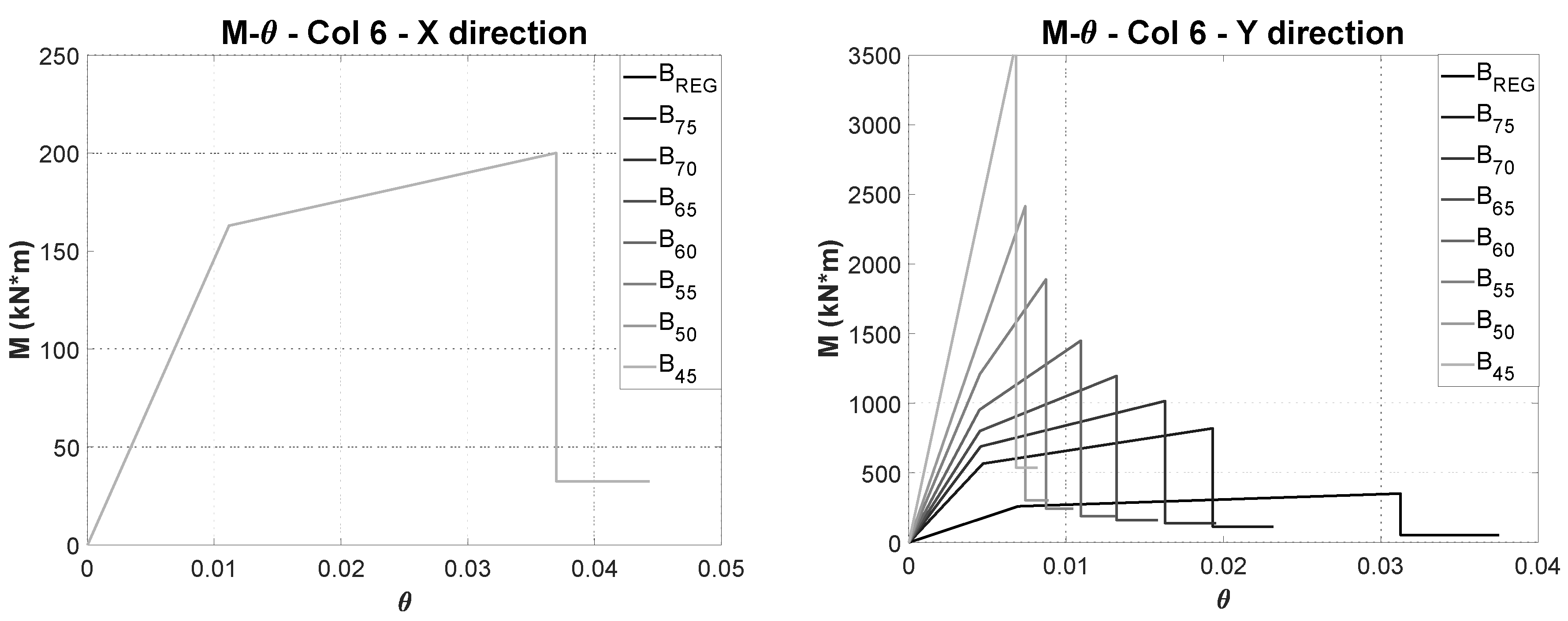
Regarding numerical models, all the 3D archetypes have been implemented in SAP2000 software [45], where beams and columns were simulated through frame elements fixed at the base through external restraints. All vertical loads were applied as distributed loads on a shell of null area, mass and stiffness and combined according to NTC2018. A rigid floor assumption has been considered for all storeys by using internal constraints. The nonlinear behaviour of the structural elements was simulated by employing a lumped plasticity approach, properly defining plastic hinges at the end of the frame sections. In particular, ductile mechanisms were accounted for by simulating a simple bending stress for the beams and for the columns a bi-directional behaviour was given by the combination of axial stress and bending. These stresses have been evaluated by considering the seismic load combination, for this reason, the constitutive law of column 6 was computed assuming a fixed axial stress. All plastic hinges are characterized by a quadrilinear constitutive law, constituted by a first branch simulating the concrete cracking, a subsequent hardening branch indicating the yielding of longitudinal steel reinforcement, a softening branch corresponding to the strength degradation of the section and a final residual moment, assumed as 20% of the yielding moment. Yielding and ultimate rotations (respectively θ_y and θ_u) were computed according to the formulation provided in the Annex of NTC2018, and the acceptance criteria were defined in terms of deformation. Confined concrete has been considered for RC sections and reduction coefficients, used for taking into account the missing efficiency of ribbed steel rebars and adequate overlap and anchor lengths, have been avoided. Limit chord rotation values have been defined in accordance with the limit-states of immediate occupancy (IO—deformation equal to θ_y), life safety (LS—deformation equal to ¾ θ_u) and near collapse (NC—deformation equal to θ_u). As previously mentioned, shear failures have been not considered. Finally, it is worth mentioning that for columns 6, at both storeys, the values of the moments and rotations in the X direction have been kept constant in all models (although strictly speaking the constitutive laws should vary), in order to avoid modifications in the structural behaviour along the X direction. Figure 3 shows the constitutive law of column 6 for all models and both directions.

By increasing the dimensions of columns 6, the nonlinear behaviour in Y direction presents an ascending overstrength increment and a descending ductility reduction.

4.2. Eigenvalue and Pushover Analyses

For the 8 numerical models, eigenvalue analysis was performed. The results in terms of the first three fundamental periods T_X, T_Y and T_θ (considering the two main translational components X and Y and the rotational one, indicated with “θ”) and the corresponding participating masses, M[%]_X, M[%]_Y and M[%]_θ, respectively, are reported in

Table 2. Modal parameters of archetype buildings.

Model	TX (s)	TY (s)	TR (s)	M[%]X	M[%]Y	M[%]R
BREG	0.3197	0.3558	0.2740	86.495	87.263	87.670
B75		0.3245	0.2507		75.061	75.861
B70		0.3194	0.2411		69.981	69.892
B65		0.3159	0.2314		65.032	64.632
B60		0.3128	0.2197		60.093	59.424
B55		0.3103	0.2045		55.056	54.212
B50		0.3077	0.1868		50.066	49.832
B45		0.3049	0.1507		44.986	44.706

.

The results show that T_X and M[%]_X remain unchanged in all numerical models, while T_Y, T_θ, M[%]_Y and M[%]_θ progressively decrease, as shown in the table. It is worth observing that for B_REG and B₇₅ the first period is the one in the Y direction (the second one is in X direction), while for the other models the reduction of T_Y causes a modal shifting, and T_X becomes the first mode.

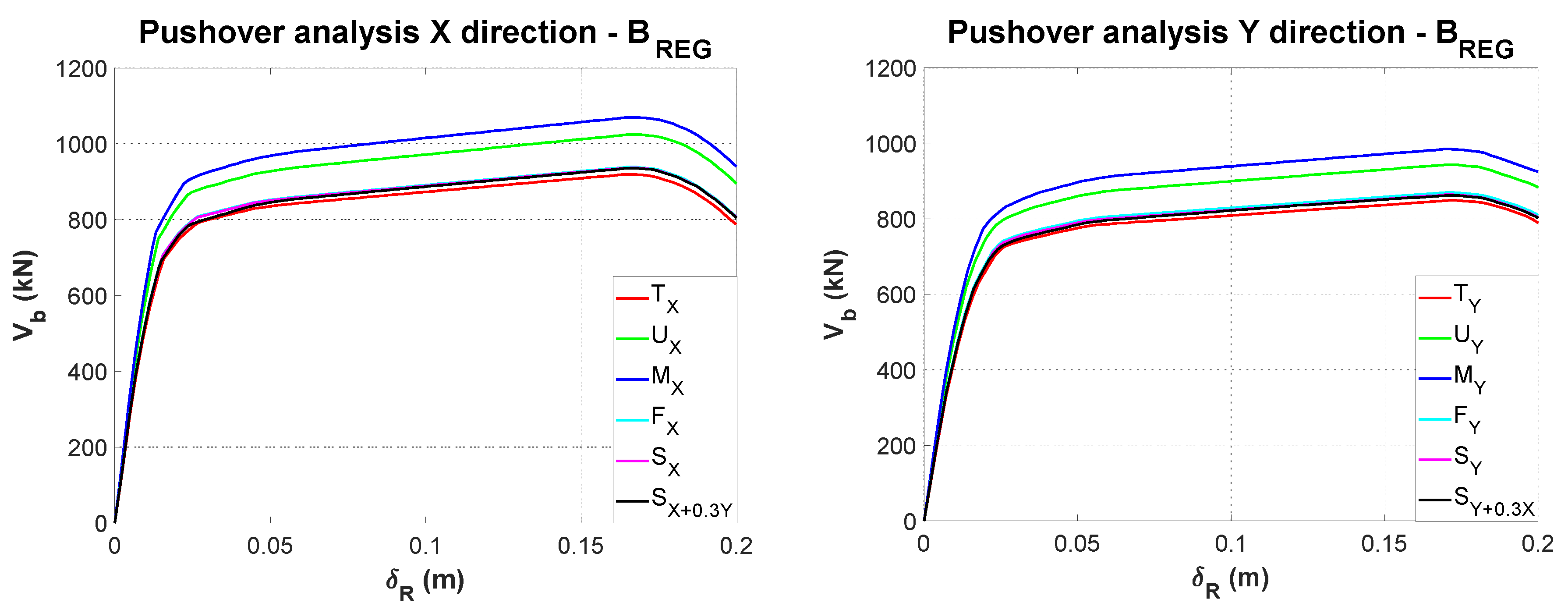
Concerning the nonlinear analyses performed, for the sake of brevity in this section we just show the pushover analyses performed for B_REG model in both directions, for all load profiles and we choose CN as the centre of masses of the last storey (Figure 4).

It is worth highlighting two aspects. Firstly, all the curves show the same structural behaviour, presenting a first reduction in overall stiffness due to the failure of beams and a final softening due to failure of the base of the columns. The global mechanism is attained for a displacement of about 18 cm, i.e., 3% of the total height of the building.

The load profiles indicated in NTC2018 (“F”, “M” and “S” mono- and bi-directional), the pushover analyses have also been performed by using “T” and “U” load profiles. If the building is regular in plan, “T” provides the same results as “F” when all floors have the same height, and U provides the same results as “M” when all floors have the same mass. Furthermore, for regular buildings (as shown in Figure 4), “S” mono- and bi-directional load profiles provide similar results to the ones obtained by “F” and “T”.

5. Discussion of Results

In this paragraph, the results of the analyses are presented and critically discussed, considering that the investigations were only performed in the Y direction, since the nonlinear behaviour along the X direction does not change. Comparisons are performed in terms of the D/C ratio at the LS limit-state (which is always lower than 1), obtained by applying the N2 method for all the models and all the load profiles (CN = node 5), as shown in

Table 3. D/C ratios for all models and capacity curves, assuming node 5 as the CN.

D/C	BREG	B75	B70	B65	B60	B55	B50	B45
TY	0.176	0.136	0.125	0.116	0.115	0.121	0.129	0.079
UY	0.153	0.12	0.108	0.096	0.101	0.105	0.112	0.068
MY	0.144	0.112	0.103	0.096	0.096	0.102	0.107	0.066
FY	0.169	0.141	0.14	0.144	0.154	0.216	0.213	0.289
SY	0.171	0.133	0.123	0.114	0.112	0.118	0.126	0.076
SX+0.3Y	0.126	0.128	0.127	0.128	0.128	0.136	0.157	0.168
SY+0.3X	0.163	0.128	0.118	0.108	0.107	0.111	0.113	0.069

.

The threshold defined for the exceedance of the LS limit-state is the achievement of a chord rotation equal to ¾ θ_u (according to NTC18) by the first element, indifferent as to whether the first element is a beam or column.

5.1. Effects of the Control Node Selection

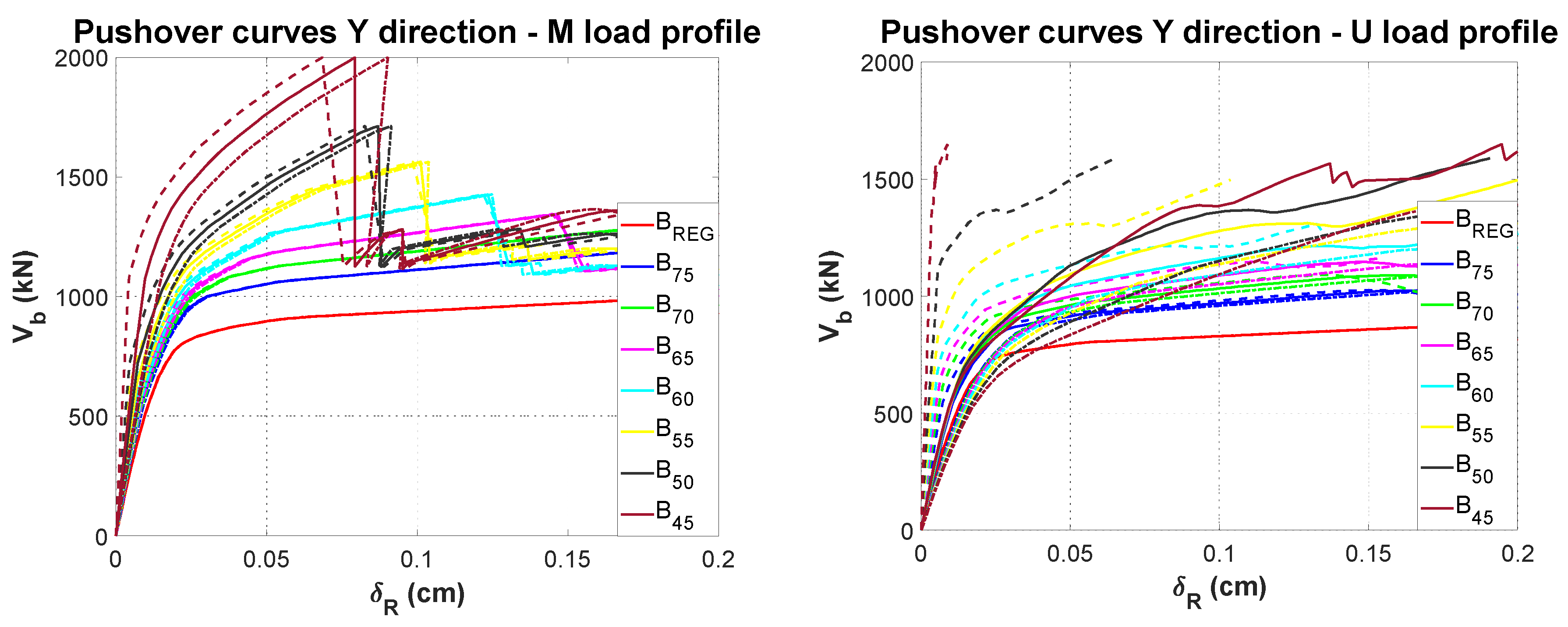
As mentioned in Section 4.1, nodes 5 (centre of the mass), 7 and 9 have been selected as CNs. Some remarks can be made about the effects of the control node variation on the Y-direction capacity curves as long as M[%] decreases in the different models. Figure 5 shows the capacity curves obtained for all models and CNs at the two load profiles “M” and “F” (the other load profiles give similar results as case “M”).

The results show that as the participating mass M[%] decreases, the curves for control nodes 7 and 9 increasingly diverge from the curve for control node 5.

This result is particularly evident for the load profile “U”, for which the variability of the pushover curves becomes very relevant. Of course, as suggested by NTC 2018 and scientific literature, the use of uniform load profiles is not recommended for buildings for which the participating mass of the first mode is less than 75%, and Figure 5 confirms this indication.

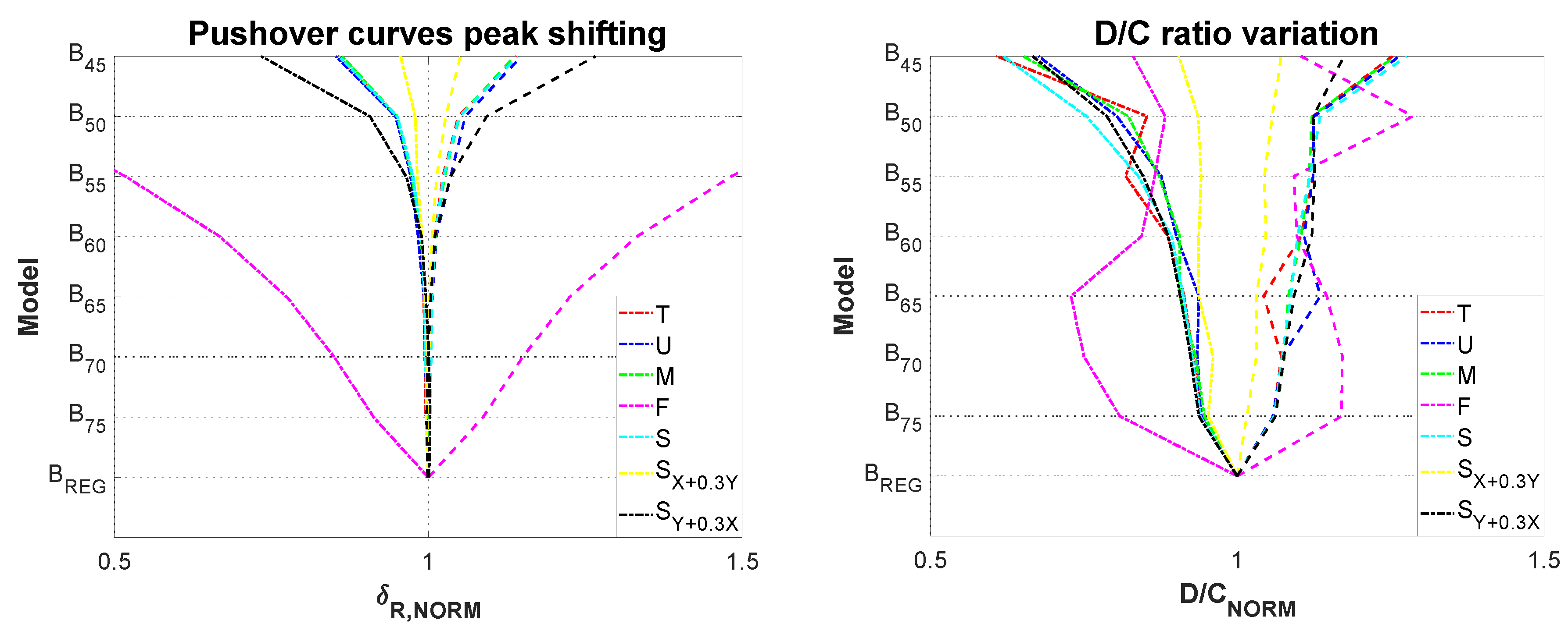
In summary, the role of the position of the NC control point in pushover analysis is described in Figure 6.

The first graph in the figure shows the trend of the maximum displacements of the capacity curves, normalized with respect to the maximum of the reference curve relative to control node 5 (δ_R,NORM), for the different load profiles and models.

Some observations can be made:

• For all load profiles, excluding F, the capacity curve peaks are invariant from the B_REG to B₆₀ models. After those models, there is an increasing divergence;
• Assuming T, U, M and S load profiles in the Y direction, the peaks are always close to the reference curve, presenting the greatest difference for B₄₅, quantifiable to about 10%;
• Assuming the S_0.3X+Y load profile, monitored in the Y direction, the peaks are more further from the reference curve, if compared with the effect shown for the above load profiles. In particular, for B₄₅ the difference can be quantified to be about 20%;
• Assuming the F load profile in the Y direction, the peaks are very far from the reference curve, achieving a difference of 50% for the B₅₅ model;
• Assuming the S_X+0.3Y load profile, monitored in the X direction, the peaks are very close to the reference curve (and to the other curves obtained by mono-directional load profiles), presenting the greatest difference for B₄₅ and quantifiable to about 5%;

More interesting from an engineering point of view is the effect on the D/C ratio, which governs the results of the assessment. In this regard, the second graph in Figure 6 shows the trend of D/C_NORM (normalized demand/capacity ratio with respect to the value relative to the reference curve), as the load profiles and models vary. It can be observed that:

• Except for the S_X+0.3Y load profile, the D/C ratios for the different models do not always follow an increasing trend and in some cases show some reversal points (e.g., the T load profile and the B₅₀ model). This is a consequence of the N2 method, the results of which are an effect of the balance between the stiffness of the single degree of freedom (SDOF) bi-linear curve and the seismic demand;
• For the load profiles “T”, “U”, “M”, “S” and “S_0.3X+Y” in the Y direction, the D/C ratios are far from the reference curve for all models, with variable differences. For B₄₅, the differences are about 15% for control node 7 and about 20 to 25% for control node 9;
• Assuming the load profile “F” in the Y direction, the differences in terms of the D/C ratio seem to have no observable systematic pattern: in some cases they are extremely conservative and in other cases they are in line with the other profiles;
• For the load profile “S_X+0.3Y” monitored in the X direction, the D/C ratios are very close to the reference curve (and to the other curves obtained with mono-directional load profiles), with greatest difference for the B₄₅ model, namely about 5 to 7%.

Finally, it can be observed that one should always monitor the point that is at the same time furthest from the centre of stiffness and furthest from the centre of the mass. In the case studies examined, point 9 fulfils this condition and provides the most conservative results.

5.2. Use of the Load Profile Proportional to Storey Shears

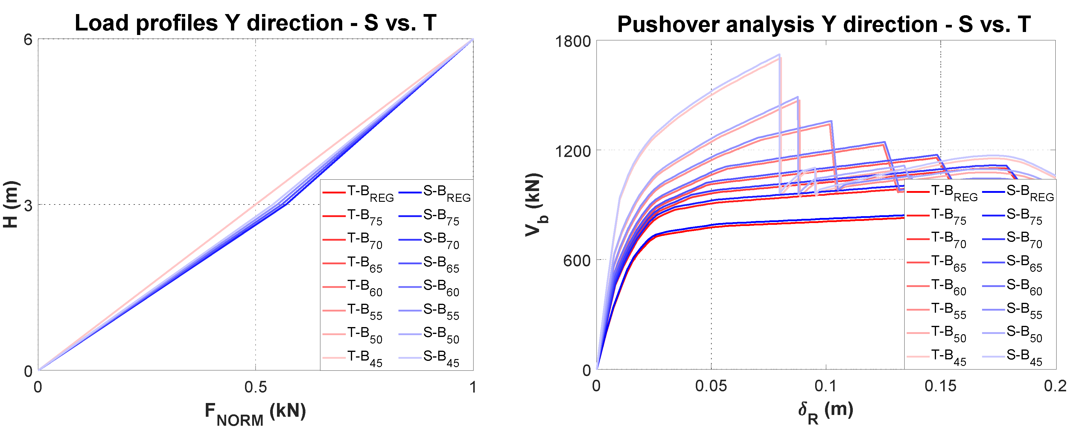
With reference to Figure 4 and Section 5.1, the results for the load profile “S” are now compared with those for the load profile “T”, for all models, and assuming CN coincides with node 5. This choice depends on two reasons: (i) “T” and “S” always provide comparable results in terms of V_b, δ_R and the D/C ratio; (ii) the shapes of the load profiles are similar for all models. Figure 7 shows, for all models, the shapes of the “S” and “T” load profiles (normalized to 1) and the related pushover curves.

As expected, the results are very similar in both cases. Only a slight variation is observed for the load profile “S” when M[%] is reduced (for the “T” profile, there is no variation) and the base shears V_b are slightly higher than in the case of the load profile “T”.

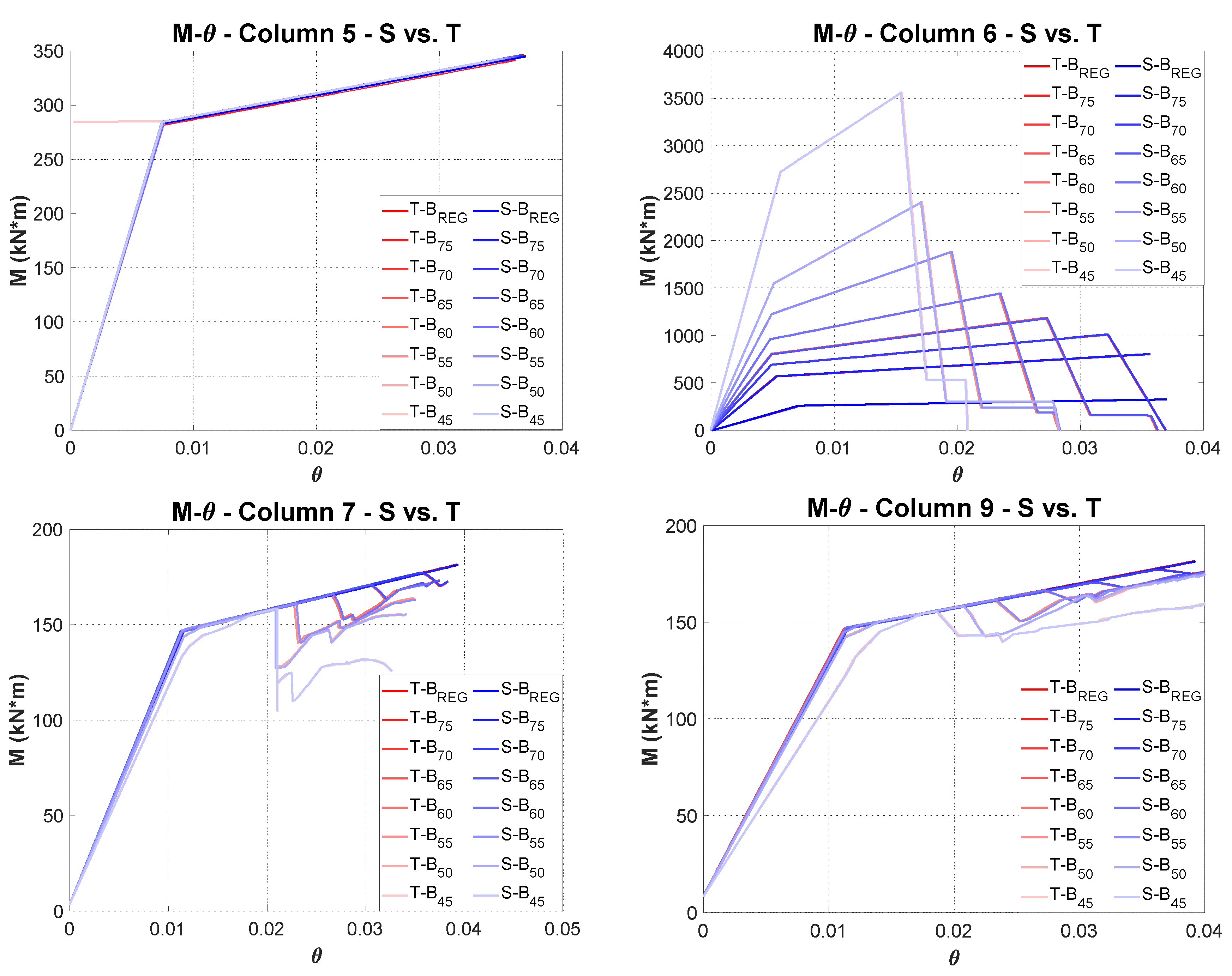
To better analyze the advantages that the use of the load profile “S” can bring to the seismic performance evaluation for the case studies, the results in terms of the moment–rotation diagram M-θ are presented for the base columns 5, 6, 7 and 9, for all models. These diagrams are shown in Figure 8.

For column 5 (which in a plan view is located at the mass centre), there are no significant variations. For column 6, the diagrams vary as the column section changes, but the two load profiles give the same results. The situation of columns 7 and 9 is different. Although some numerical convergence problems are evident, the stiffness variations are small for models up to B₄₅, after which they become larger. No difference can be observed, even here, between the load profiles “S” and “T”.

The general framework of the analyses carried out and, in particular, the results depicted in Figure 7 and Figure 8, suggest that the load profile “S” does not provide results different from those obtained from the load profile “T”. In this regard, it is worth noting that the main advantage of an RSA (compared to a linear static analysis) is to take into account the torsional effects, which in any case do not affect the global storey shear. While in fact, the additional torsion can vary the stress states in the single structural elements (it increases the shear in the lateral columns and reduces the shear in the central ones), it does not vary the resultant of the shears of all the structural elements at the storey. For this reason, at least in the models examined, the load profile “S” does not bring evident improvements to a simple and well-known load profile “T”. No differences are also evident at the local level of individual columns. In addition, observing the evolution of the load profiles “S” in Figure 7, it can be concluded that this new indication of NTC 2018 does not really seem useful in the case of in-plan irregularity. In the case of in-elevation irregularity, a situation that could strongly change the shape of the “S” profile, the use of this profile could perhaps be useful, but this aspect needs to be further investigated.

5.3. Application of Bi-Directional Pushover Analysis

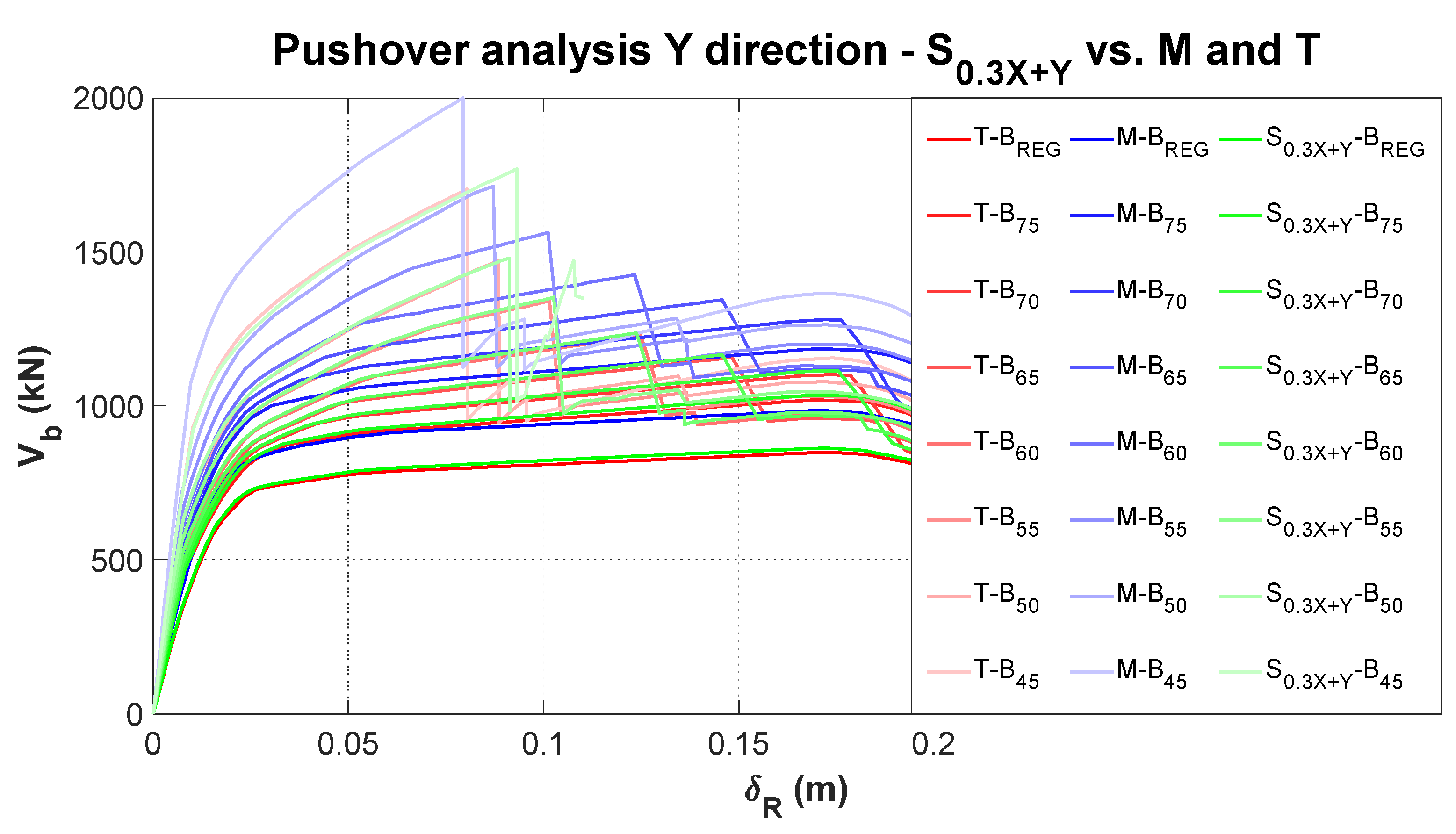
The use of bi-directional pushover analysis for the seismic assessment is now investigated and compared with the mono-directional ones. The different pushover curves obtained for the models are shown in Figure 9, where the S_0.3X+Y profile is compared with the “T” and “M” profiles, which are those that showed the widest return range of variation in the pushover response (see Figure 4, post-elastic branch of the pushover curves).

The plots shown in the figure suggest some considerations about the variation of the results obtained with the “S_0.3X+Y” profile for the various models.

For regular models, the curves are comparable with those relative to the load profile “T”, while for irregular models, “S_0.3X−Y” gives a slightly different value of the base shear V_b, with displacement higher than that of the “T” profile. With regard to load profile “M”, several differences can be observed, in particular an increasing difference in terms of V_b.

In view of the seismic assessment, it is appropriate to express the results in terms of the D/C ratio, shown in Table 3. The values obtained for the “S_0.3X+Y” profile are always between those obtained by “T” (higher values) and “M” (lower values). If a conservative approach is taken, “T” would seem to be the most appropriate profile. The results for the “S_0.3X+Y” profile could be more accurate, but this should be further investigated and validated by non-linear dynamic analyses and by extending the building sample.

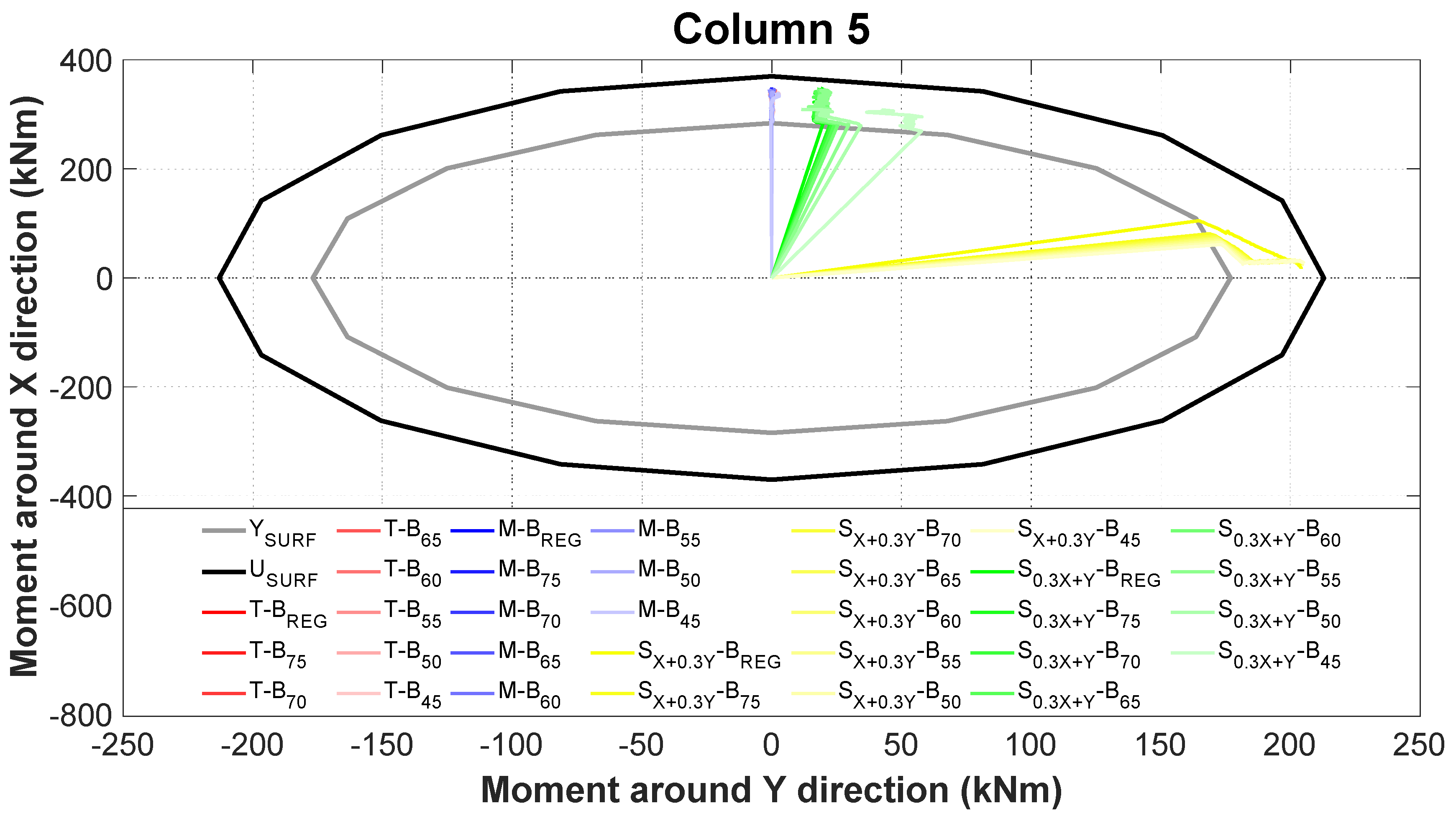
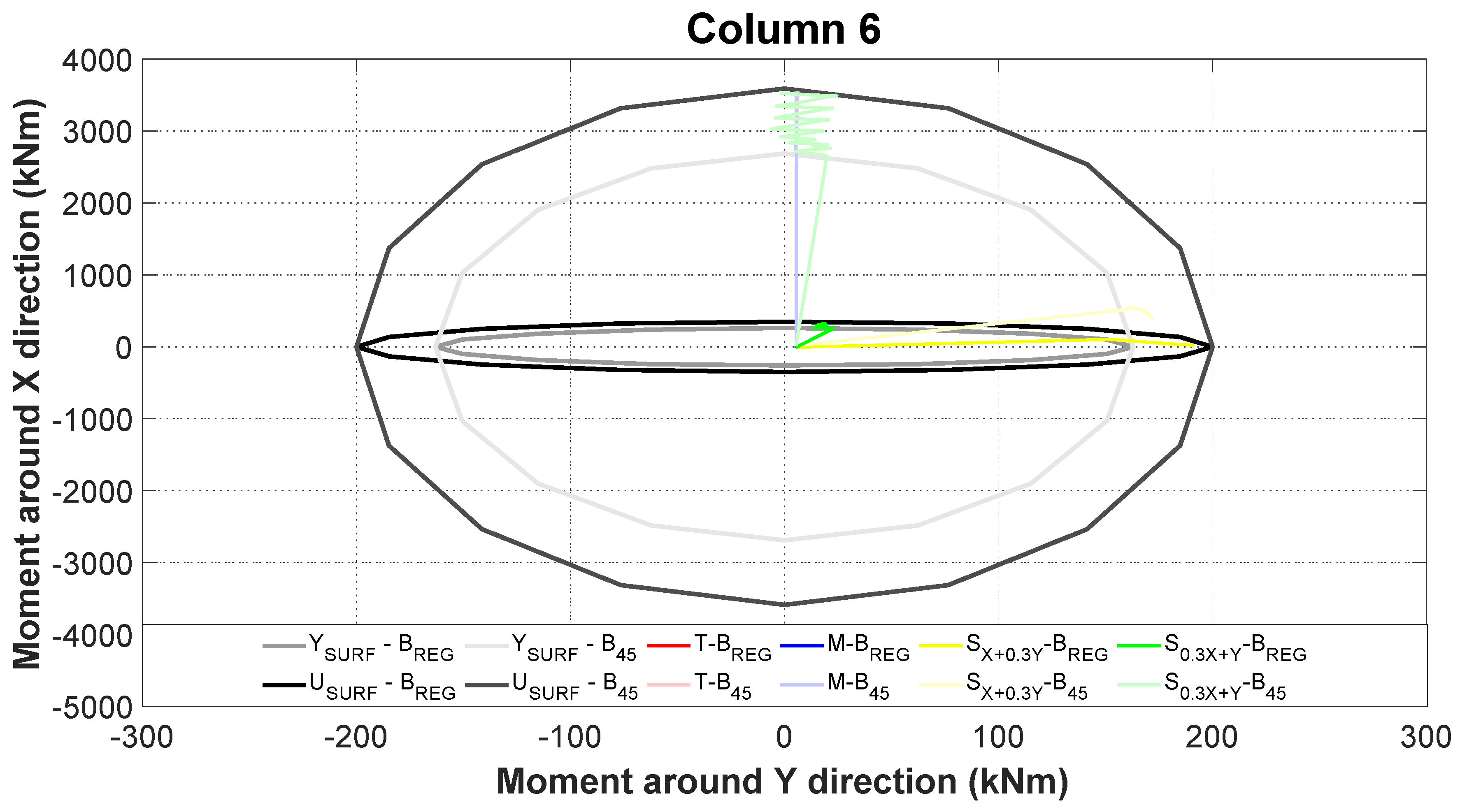
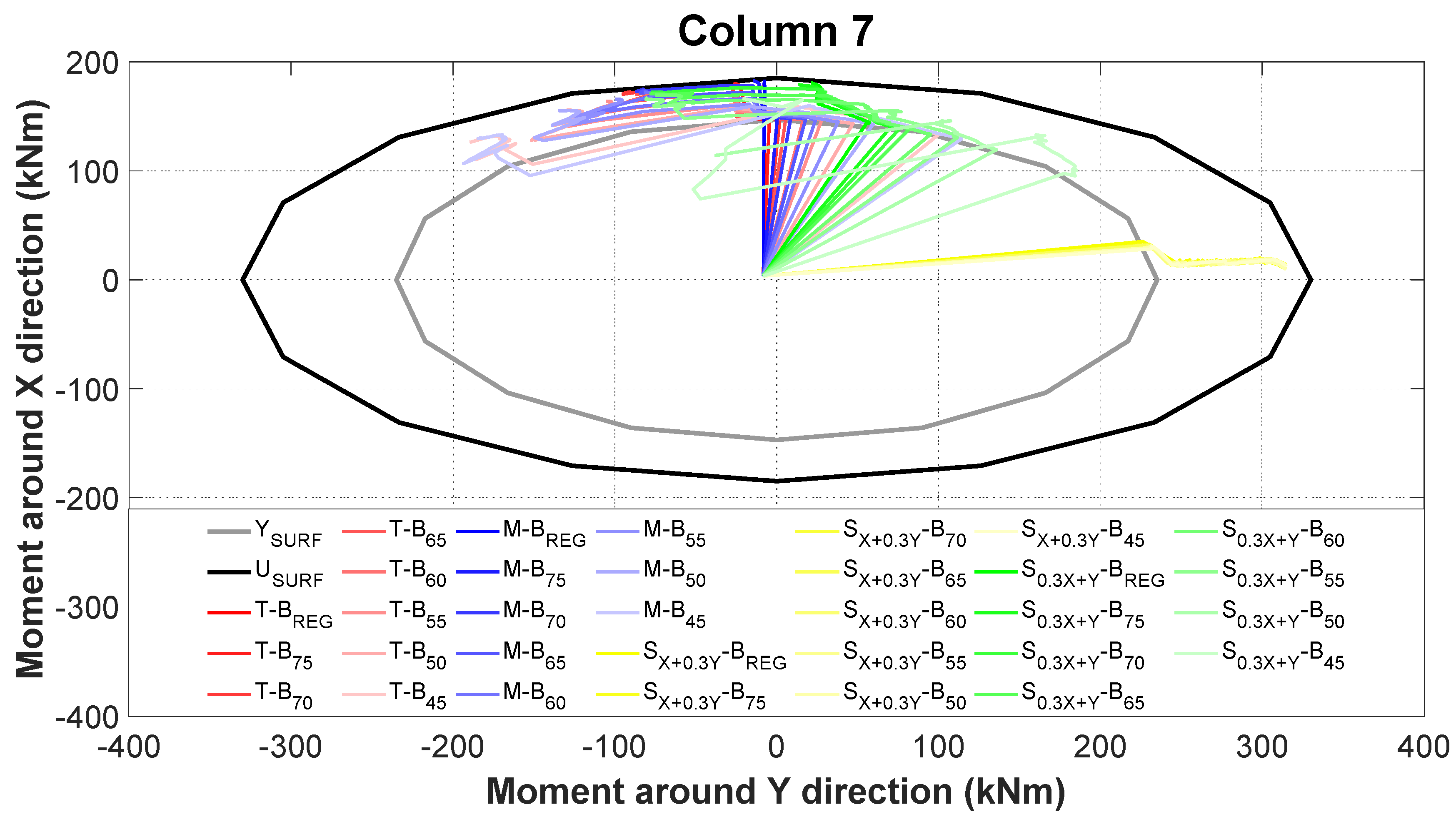
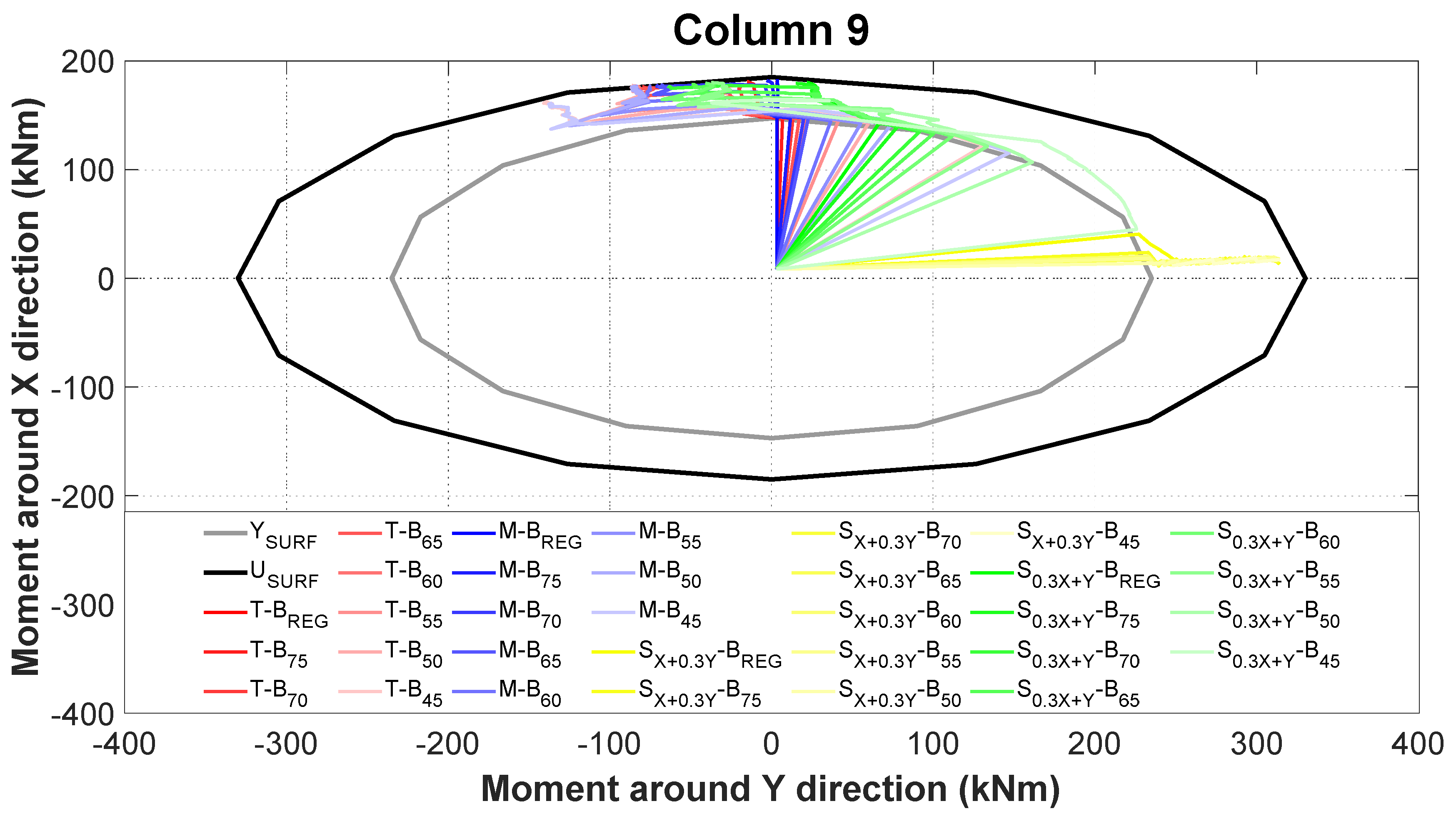
At a local level, it is interesting to analyse how the base columns behave under the bi-directional pushover. In this regard, for columns 5, 6, 7 and 9, the M_X–M_Y interaction domains are reported, respectively, in Figure 10, Figure 11, Figure 12 and Figure 13.

The axial stress considered is invariant (it corresponds to the seismic combination, coherently with the plastic hinges) and shows the yielding and ultimate limit surfaces. On the graphs, the actual path followed during the load history is reported for the different pushover cases (“T”, “M”, “S_X+0.3Y” and “S_0.3X+Y” load profiles) and varying the numerical models. It is worth noting that, for column 6, both yielding (Y_SURF) and ultimate (U_SURF) moment surfaces are variable in the Y direction. Of course, there would also be a variation in the X direction, which has been neglected since it is not as significant as the Y variation. Figure 11 reports only the two surfaces corresponding to B_REG and B₄₅.

Before discussing the results obtained, it is worth mentioning that all the curves plotted do not start from the origin, due to the nonlinear application of vertical loads.

Some remarks can be made about Figure 10, Figure 11, Figure 12 and Figure 13:

• With regard to column 5, which is coincident with the centre of the masses, the mono-directional pushover analyses in the Y direction always follow the same direction, whereas the bi-directional analyses reach the yield surface Y_SURF with a different slope and in the post-elastic field the paths are parallel to the dominant component of the load profiles (both for the X and Y directions);
• In column 6, which is the column that is progressively modified in the different models, the mono-directional pushover analyses in the Y direction follow this same direction. For the bi-directional analyses, in the elastic branch a slope variation can be observed depending on the variation of the column section. In the Y-direction, the variation is more evident than in the X-direction, with a post-elastic behaviour disturbed by numerical convergence problems;
• With regard to columns 7 and 9, which are the columns with the greater displacements, both mono- and bi-directional pushover analyses have different slopes in the elastic field, due to the increasing torsion. In general, in the post-elastic field, the path tends to re-align to the direction of the dominant component of the load profiles, but due to the presence of numerical convergence problems, this happens with no recognizable rule. Probably, in these two columns, the results obtained are actually governed by the high variability of the axial load.

In conclusion, and on the basis of the local response of some columns, the use of “bi-directional” pushover analysis does not seem to provide a conservative approach for the seismic assessment of existing RC buildings. On the other hand, such an approach could be more accurate than a “conventional” pushover analysis with regard to the effects of the spatial variability of seismic motion. Obviously, such a conclusion needs to be supported by a comparison with the results of an extensive campaign of non-linear dynamic analysis.

6. Conclusions and Future Developments

This study presents an investigation of new trends about conventional pushover analysis in the latest release of the Italian Building Code, with a particular reference to the effects of the spatial variability of seismic action, which are usually investigated through nonlinear dynamic analyses.

The new prescriptions about nonlinear static analysis that have been examined concern: (i) the use of additional control nodes; (ii) the possibility of using a load profile proportional to the storey shears obtained from an RSA in all cases; and (iii) a combination of the spatial effects with an approach similar to the procedure used for RSA.

To assess the actual benefits of these indications, a set of eight low-rise RC archetype buildings has been generated and investigated. The first reference model is extremely regular and was designed following the rules of capacity design. Additional models were generated by modifying the centre of stiffness to produce an increasing irregularity in-plan. All the models have been investigated by using several load profiles and by analysing the results in terms of global and local response and safety level parameters (D/C ratio). The results obtained are listed below:

• The use of different control nodes in the analyses, varying models and load profiles, has provided a large set of capacity curves. It is interesting to look at the variations obtained in view of the selection of the most conservative choice in terms of safety level, even if this is in contrast with the spirit of a non-linear analysis, which is supposed to be accurate rather than cautious. In this sense, anyway, the more convenient result is given by the control node that is the farthest from the centres of mass and stiffness;
• The use of the “S” load profile deriving from an RSA analysis has not given significant differences from a classic “T” load profile in any numerical model. This evidence cannot be generalized, but seems to suggest that possibly the “S” load profile could be very useful in the case of buildings presenting irregularities in-elevation, which deserves further investigation;
• The use of bi-directional pushover analyses has been tested in order to fulfil the new indication of the Italian law about the spatial combination of effects. It seems to provide some benefits, since it offers the possibility to investigate how structural elements behave under the spatial effects of ground motion. On the other hand, with regard to the classical pushover approach, it does not provide a conservative approach, since the response is between the extreme load profiles. This solution could be more precise, but this should be validated with more accurate spatial analyses.

Considering that the sample investigated is still limited, the conclusions of this paper cannot be generalized to all cases of new and existing buildings and, for this reason, future researches will aim to extend the sample of cases to investigate and compare the pushover analysis results with the ones obtained by nonlinear dynamic analyses.