A Durability Prediction for the Magnesium Alloy AZ31 based on Plastic and Total Energy

Abstract

Magnesium has a good strength-to-weight ratio. As a result, magnesium alloys are gradually becoming an integral part of lightweight designs that are especially important to the automotive and aerospace industries. The magnesium alloy AZ31 is particularly suitable for forming. Furthermore, as its cyclic response is asymmetric, the accumulated energy during loading is a convenient basis for durability predictions of a product that is made of the AZ31 alloy. In this article, we show how the inverse-power law model can be combined with a Weibull’s probability density function to describe the shape of the fatigue-life curves and their scatter. Various load histories were chosen to characterize the response of the AZ31 alloy under different cyclic loadings. Both the plastic and the total strain energy densities were calculated for all the load histories, and then, a suitable dependence in terms of energy fatigue-life curves was determined. The proposed model is appropriate for modeling the low-cycle fatigue life of the AZ31 alloy. With the application of a linear damage-accumulation rule, it is also possible to predict the fatigue life for the non-constant amplitude loading within one decade of accuracy.

1. Introduction

Nowadays, most of the load-carrying structures and structural components are subjected to dynamic loads. A typical mode of failure for repetitive (dynamic) loading is the fatigue of a material, which eventually leads to the rupture of structural components. Basically, there are two kinds of fatigue phenomena. If the stresses due to the dynamic loading are less than the material’s yield stress, no plastic phenomena occur during the loading. In this case, the structure fails due to a large number of repetitive loading cycles and the phenomenon is called high-cycle fatigue. On the other hand, if the stresses due to the dynamic loading of the structure surpass the material’s yield stress, the structure fails after a relatively small number of loading cycles and the failure is called low-cycle fatigue. In the low-cycle-fatigue regime, the cyclic elastic-plastic response of the applied material governs the fatigue process. In order to effectively design reliable structures for a target fatigue life, the engineering fatigue-life properties of the applied material must be known.

One of the solutions to reduce the carbon footprint during road transport is to make the means of transport lighter in weight. Various types of magnesium alloys represent good alternatives for producing lightweight structures. However, due to the crystallographic characteristics of magnesium and its alloys, the elastic-plastic stress-strain responses in tension and compression are not equal. In our research, the focus was on the AZ31 magnesium alloy, because it is one of the most promising magnesium alloys for serial production [1]. To make the industrial application of such an alloy possible, its fatigue behavior must be known. A structural material is usually supplied in the form of half-products, i.e., sheet plates, rods, extruded profiles, etc., of different sizes. In the case of the AZ31 magnesium alloy the half products are often produced by hot forming procedures that may be followed by heat treatment, since a ductility of this alloy at the room temperature is rather poor. With the additional processing technologies (e.g., equal channel angular pressing [2,3]) the mechanical characteristics of the half-products can be significantly improved. Nevertheless, it was decided to use the sheet-plate half products as supplied without additional processing in our case. This is because such material is widely commercially available, which is important for engineering applications.

In practice, many different approaches to calculating a structure’s fatigue life exist. Due to the asymmetric AZ31 hysteresis loops, we chose to follow the energy approach for estimating the low-cycle fatigue life of this alloy. One of the simplest and first-introduced energy-based criteria for the fatigue-life prediction in the low-cycle and high-cycle fatigue domains is the Smith-Watson-Topper approach [4]. Although this approach works well for metals with symmetric elastic-plastic hysteresis loops, its use for materials with asymmetric hysteresis loops is questionable. That is why we decided to follow a methodology that considers the true dissipated energy during the cyclic loading when predicting the fatigue life of the magnesium alloy AZ31.

In the low-cycle-fatigue regime the fatigue life is influenced by both the dissipated (plastic) strain-energy density ΔW_p and the elastic strain-energy density ΔW_e of the loading cycle [5]. Different energy approaches vary mainly according to the methodology of calculating the elastic strain-energy density ΔW_e in order to consider the mean-stress effect in the appropriate way [6,7,8,9,10,11,12,13,14,15,16,17]. A special loading case is a fatigue loading with tensile pulsating loading cycles. When the AZ31 alloy is exposed to such loading history a significant damage contribution results from a large plastic deformation in the first loading cycle. For this reason, Park et al. [18] added an additional term to the cyclic strain energy density to account for this effect.

After the strain-energy density of the closed loading cycle ΔW is calculated, the corresponding fatigue-life dependency ΔW–N_f needs to be determined. The simplest approach to estimating the ΔW–N dependency is based on the idea that the same amount of strain-energy density is needed for the fatigue-life rupture as for the static tensile rupture. This means that the predicted number of loading cycles to failure N_f is equal to the quotient of the strain-energy density calculated from the tensile test and the strain-energy density of the loading cycle ΔW [19,20]. Oftentimes, this approach is too general, and its fatigue-life predictions are poor. For this reason, the inverse-power-law equation that links the strain-energy density ΔW to the number of loading cycles to failure N_f is normally applied [15,21,22]. We decided to follow the approach of Park and Nelson [15], since this approach or its variations were already successfully applied in the past for calculating the fatigue lives of different magnesium alloys [10,11,22,23,24].

In our research, a series of constant-strain amplitude fatigue tests were performed to establish a dependency between the strain-energy density of the cyclic loading and the corresponding fatigue life. Due to the significant scatter of the fatigue-life data the ΔW–N_f fatigue-life curve was modeled with a conditional Weibull’s probability density function in the same manner as in the case of the S-N and E-N fatigue-life curves [25,26,27]. After the ΔW–N_f fatigue-life curve and its scatter were estimated for the constant strain-amplitude data, the applicability of a linear-damage-accumulation rule in combination with the energy approach was then assessed for a series of strain-controlled step-strain fatigue tests and random-amplitude fatigue tests.

The article is structured as follows. In the second section the material data and the theoretical background of the applied energy method for calculating the fatigue life are explained together with the model of the energy durability curve and its scatter. The experimental and modeled results are presented in the third section, which is followed by a discussion in the fourth section. The article is concluded with a brief summary, acknowledgments and a list of references.

2. Materials and Methods

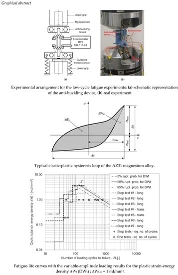
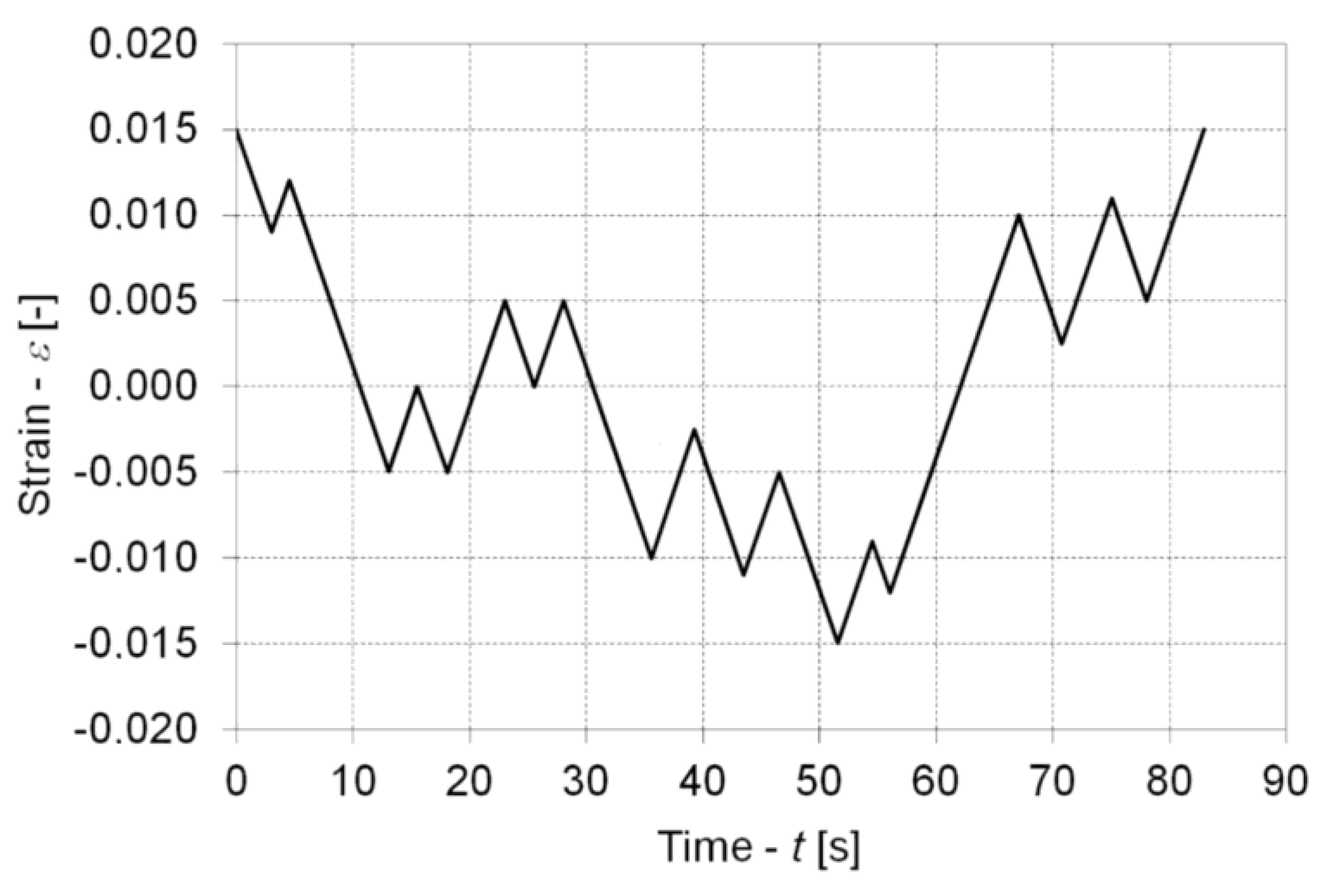
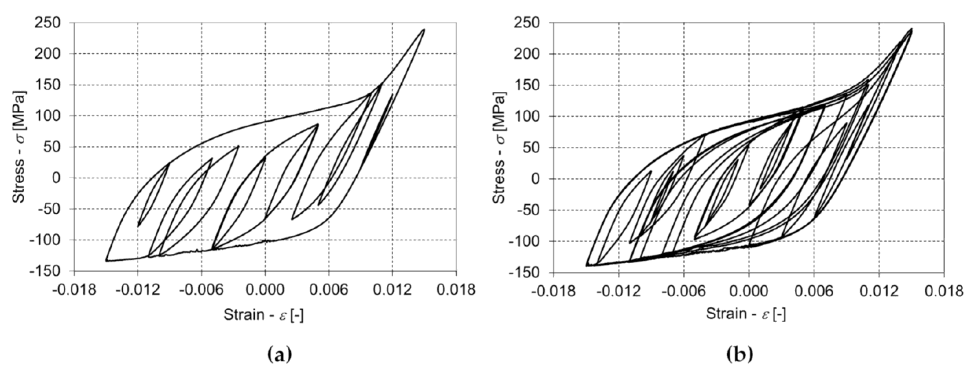
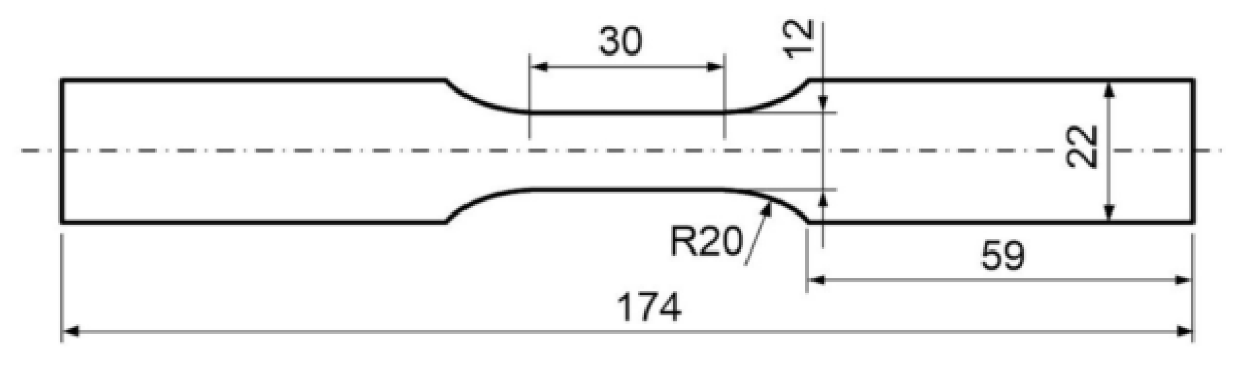
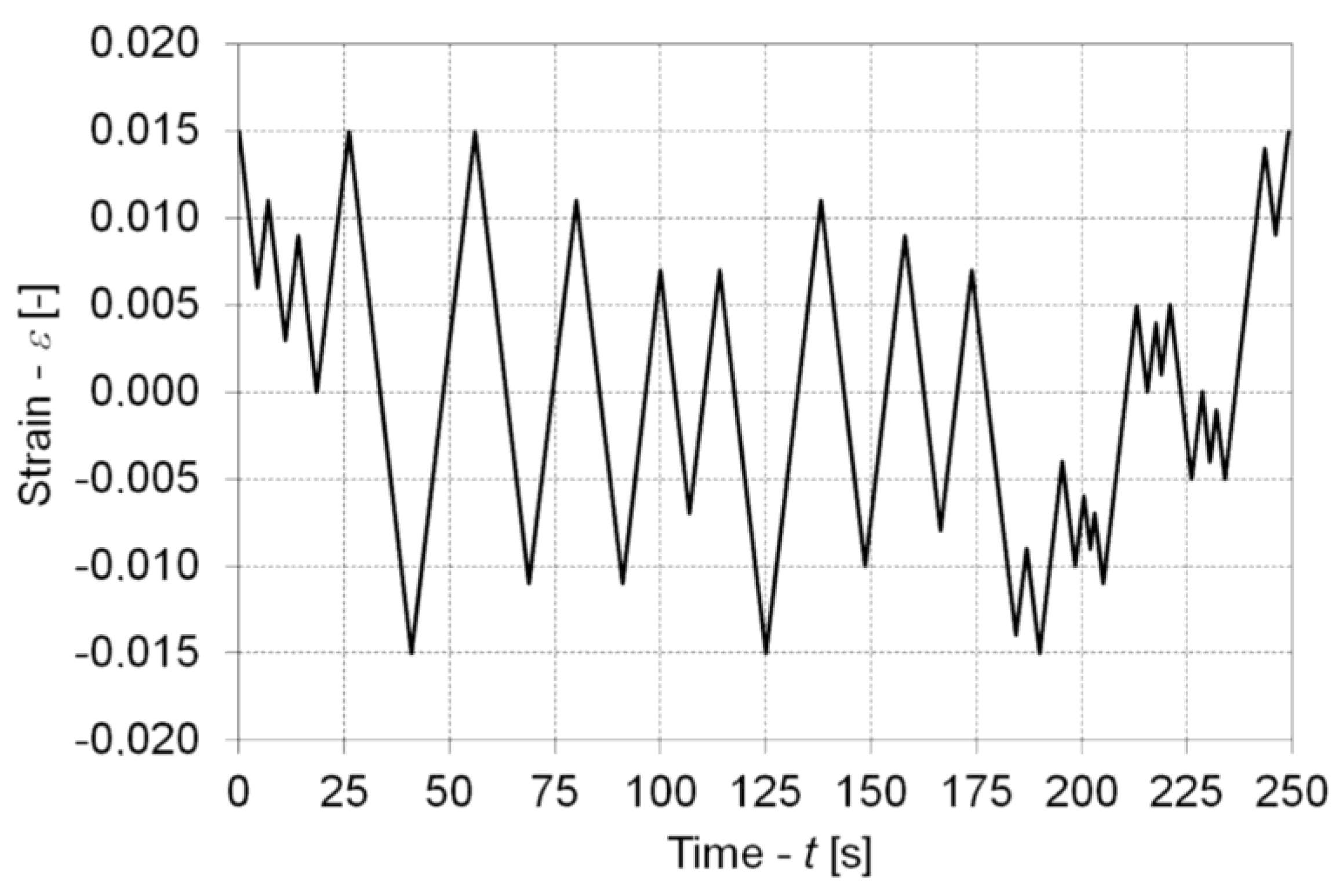
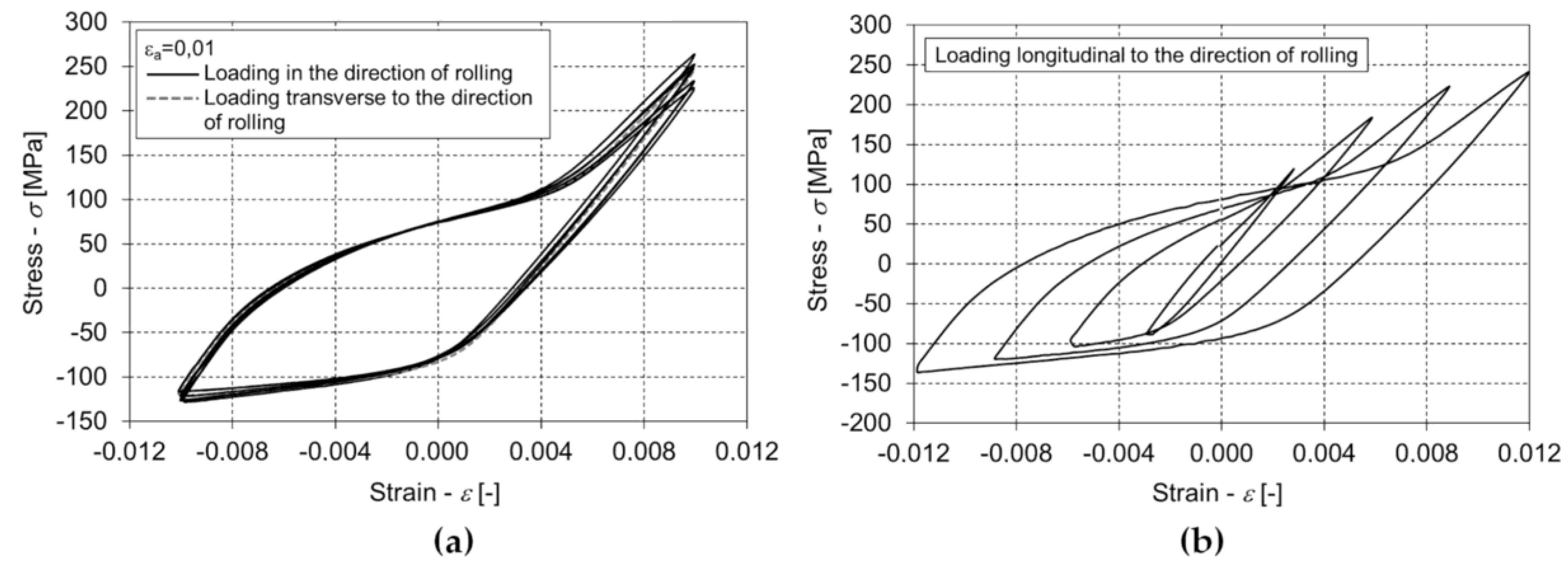
2.1. The Magnesium Alloy AZ31 and the Low-Cycle Fatigue Experiments

The material under investigation was the magnesium alloy AZ31. The bulk chemical composition of the alloy is 96% Mg, 3% Al and 1% Zn. The specimens for the low-cycle fatigue-life experiments were cut from the hot rolled 2-mm-thick sheet plates of the AZ31 alloy with dimensions of 200 mm × 200 mm. The sheet plates from two different production series, which were supplied by Goodfellow Cambridge Ltd. (Huntingdon, UK), were not additionally mechanically or heat treated to improve their properties. As reported by the supplier, the elastic modulus of the AZ31 alloy is E = 45 GPa, the ultimate tensile strength R_m = 290 MPa, the elongation at break is 15%, the density ρ = 1800 kg/m³ and melting temperature is 605–630 °C [28]. To check the basic material properties, four tensile tests with the specimens from the first production series were performed on a Zwick/Roell Z50 testing machine (ZwickRoell, Ulm, Germany) using the dog-bone specimens illustrated in Figure 1. For the tensile tests the specimens were fine cut with a water-jet machine in the direction of rolling (longitudinal direction) as well as perpendicular to the rolling direction (transversal direction). The average elastic modulus from the tensile tests was E = 44.1 GPa, with a standard deviation of 0.8 GPa. The average measured ultimate tensile strength was R_m = 253.4 MPa with a standard deviation of 2.6 MPa, and an average elongation at break equal to 18.7%, with a standard deviation of 3.5%. When compared with the reported data, the supplied sheet plates of the AZ31 alloy are more ductile with a lower strength. In Figure 2a, a microstructure after a tensile load is presented. In Figure 2b, a microstructure structure after few completed loading cycles of constant strain amplitude is presented. The picture orientations were parallel to the mid-plane of the specimen. Microstructure observations were carried out on a light microscope Olympus BX61 (Olympus, Tokyo, Japan). It can be seen from Figure 2 that the average grain size is approximately between 20 and 30 µm and the grains are not elongated in either of the two specimen directions, i.e., longitudinal or transversal.

For the low-cycle fatigue experiments the specimens as presented in Figure 1 were fine cut with a water-jet machine in the longitudinal and transversal directions. These specimens originated from two different supplied series. The low-cycle fatigue-life experiments were carried out on a 100-kN MTS hydraulic machine (MTS, Eden Prairie, MN, USA) and were strain-controlled. The strains were measured with an MTS 834.11F-24 extensometer (MTS, Eden Prairie, MN, USA) and the force was measured with a 100-kN tensile-compressive load cell (MTS, Eden Prairie, MN, USA). Our own-developed anti-buckling device was used to solve the stability issues during the experiments. The low-cycle fatigue experimental arrangement is presented in Figure 3. The anti-buckling device prevents buckling along the weak axis of the specimen, but not along the strong axis. It is attached to the lower grip of the testing machine using two springs that ensure a continuous contact between the device and the sensor, which measures the friction between the specimen and the guiding surface of the device. Between the specimen and the guiding surface there is a thin teflon foil of 0.1 mm thickness. The contact pressure between the specimen and the guidance is negligible until the instability of the specimen occurs. The details of measuring the friction between the specimen and the anti-buckling device, together with some experimental results for different materials, can be found in the literature [29,30].

The low-cycle fatigue experiments were all strain controlled. The constant-amplitude experiments and the step-strain low-cycle fatigue experiments were fully reversal according to the strains ε. The constant-amplitude experiments were performed for the following strain-amplitude levels ε_a: 0.25%, 0.4%, 0.5%, 0.6%, 0.75%, 0.9%, 1.0% and 1.25%. For each strain-amplitude level at least one experiment was conducted. The testing frequency depended on the strain amplitudes and was in the range between 0.1 and 1.0 Hz. Altogether, 16 constant-amplitude experiments were carried out in order to obtain the strain-energy density fatigue-life curves.

The step-strain low-cycle fatigue experiments were different according to the starting strain level, the strain increment between the consecutive steps and the number of loading cycles within a single block. Each step-test was finished after the rupture of the specimen. The testing frequency range was the same as for the constant-amplitude experiments. Altogether, eight step-tests were carried out. The details of the step-strain experiments are listed in

Table 1. Step-strain low-cycle fatigue experiments.

Test No.	Specimen Orientation	Strain Levels - εa (Number Of Loading Cycles in Blocks - N)
1	longitudinal	${\epsilon }_{\mathrm{a},1}=0.1\%$ ($N_1=20$)	${\epsilon }_{\mathrm{a},2}=0.25\%$ ($N_2=20$)	${\epsilon }_{\mathrm{a},3}=0.5\%$ ($N_3=70$)	${\epsilon }_{\mathrm{a},4}=0.75\%$ ($N_4=110$)	${\epsilon }_{\mathrm{a},5}=1.0\%$ ($N_5=$ rest)
2	longitudinal	${\epsilon }_{\mathrm{a},1}=0.1\%$ ($N_1=3$)	${\epsilon }_{\mathrm{a},2}=0.25\%$ ($N_2=3$)	${\epsilon }_{\mathrm{a},\mathrm{i}}={\epsilon }_{\mathrm{a},\mathrm{i}-1}+0.25\%;i=3,4,\dots$ ($N_{\mathrm{i}}=3;i=3,4,\dots$)1
3 4 5 6	longitudinal longitudinal transversal transversal	${\epsilon }_{\mathrm{a},1}=0.05\%$ ($N_1=20$)	${\epsilon }_{\mathrm{a},2}=0.1\%$ ($N_2=20$)	${\epsilon }_{\mathrm{a},3}=0.25\%$ ($N_3=20$)	${\epsilon }_{\mathrm{a},\mathrm{i}}={\epsilon }_{\mathrm{a},\mathrm{i}-1}+0.25\%;i=4,5,\dots$ ($N_{\mathrm{i}}=20;i=4,5,\dots$)1
7	longitudinal	${\epsilon }_{\mathrm{a},1}=0.25\%$ ($N_1=40$)	${\epsilon }_{\mathrm{a},2}=0.75\%$ ($N_2=40$)	${\epsilon }_{\mathrm{a},3}=1.25\%$ ($N_3=$ rest)
8	longitudinal	${\epsilon }_{\mathrm{a},1}=0.3\%$ ($N_1=30$)	${\epsilon }_{\mathrm{a},2}=0.6\%$ ($N_2=30$)	${\epsilon }_{\mathrm{a},3}=0.9\%$ ($N_3=30$)	${\epsilon }_{\mathrm{a},4}=1.2\%$ ($N_4=$ rest)

¹ Loading levels were incremented up to failure.

.

Two random-loading fatigue tests were also carried out to check the applicability of the energy approach in practice. The blocks of the random strain time series, which are presented in Figure 4 and Figure 5, were repeated until the rupture of the specimen. As can be seen in the two figures, the transition between the consecutive reversal points was linear with a constant strain rate of 0.2%/s. The outcomes of all the presented low-cycle fatigue experiments are available as a supplement Excel workbook in the Supplementary Materials.

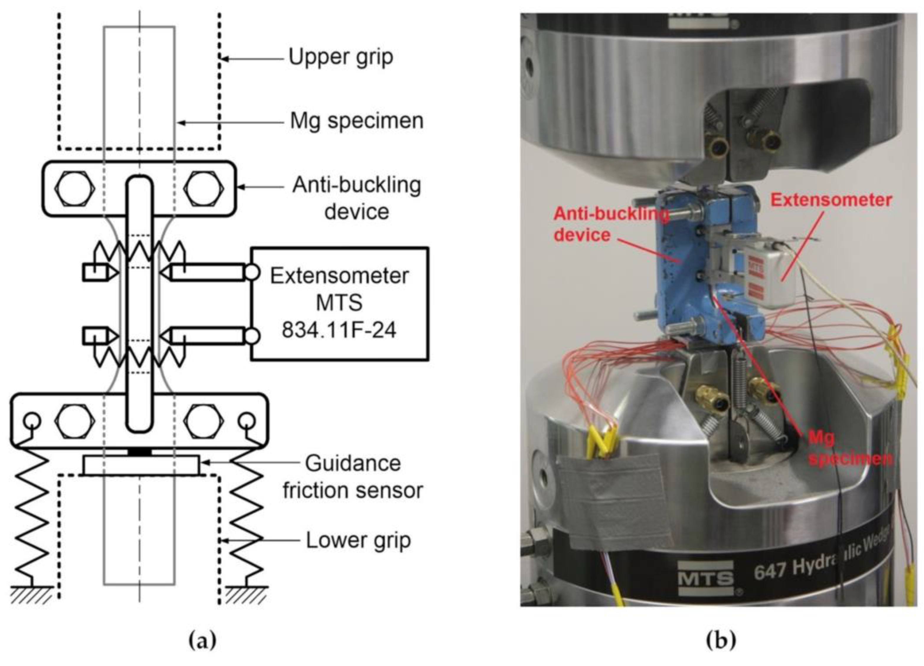
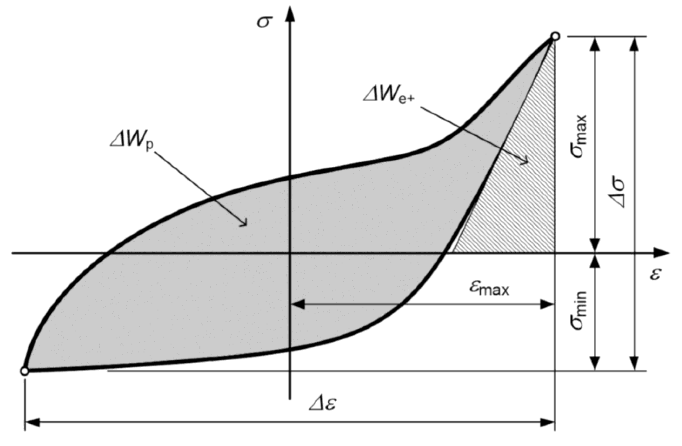
2.2. Calculating the Fatigue Damage on the Basis of the Strain-Energy Density

When following the most simple Smith-Watson-Topper approach [4], the strain-energy density of a closed loading cycle ΔW is defined as a rectangle in the σ-ε space, i.e., $\Delta W={\sigma }_{\max }\cdot {\epsilon }_{\mathrm{a}}$. σ_max is the maximum stress of the loading cycle and ε_a is its strain amplitude. The fatigue life is predicted on the basis of the strain-energy density ΔW–N_f durability curve that is derived from the Coffin-Manson equation. N_f represents the number of repeated loading cycles to failure at the corresponding ΔW level. In this case the strain energy density of the loading cycle ΔW is not divided to the contributions of plastic (ΔW_p) and elastic (ΔW_e) strain energy densities.

By following the true strain-energy density concepts, the plastic strain-energy density ΔW_p is always calculated in the same way. However, there are many different approaches to calculating the elastic strain-energy density ΔW_e in order to weight the mean-stress effect in the appropriate way. Usually, the elastic strain-energy density ΔW_e is only defined for positive strain values. If the stress-related dynamic loading factor R_σ is negative the elastic strain energy is the surface of the triangle in the σ-ε space below the compressive loading path for positive stresses—see Figure 6. If the minimum stress σ_min is positive (R_σ > 0), different formulations of the elastic strain-energy density ΔW_e were defined in the past [6,7,8,9,10,11,12,13]. Sometimes, the elastic energy density is calculated for both the compressive and tensile loading paths [14,15], and sometimes, it is calculated in a similar manner to the Smith-Watson-Topper approach [16,17].

When dealing with the total strain-energy density as a criterion for predicting the fatigue life, we decided to follow the approach of Golos [6,7] and Koh [8], because it is relatively simple and yields reasonable results [9]. When combining these approaches the total strain-energy density ΔW_t is the sum of the plastic strain-energy density and the tensile elastic strain energy, as presented in Figure 6:

$$\Delta W_{\mathrm{t}}=\Delta W_{\mathrm{p}}+\Delta W_{\mathrm{e}+}$$

(1)

In our research the additional term of Park et al. [18] that considers the influence of the large plastic deformation in the first loading cycle to the accumulated damage was not considered. This is because our loading was fully reversal according to strain – R_ε = −1 (this also holds for the stress-strain envelope of the random loading), thus, this term would have no effect to the calculated fatigue damage.

The plastic strain-energy density ΔW_p of a closed hysteresis loop is calculated as:

$$\Delta W_{\mathrm{p}}={\displaystyle \int \sigma (\epsilon )\cdot d\epsilon }$$

(2)

The elastic strain-energy density ΔW_e+ of a tensile elastic part that corresponds to the closed hysteresis loop of a loading cycle is calculated as:

$$\Delta W_{\mathrm{e}+}=\{\begin{array}{l}\frac{{\sigma }_{\max }^2}{2\cdot E};{\sigma }_{\min }\le 0\\ \frac{{\left({\sigma }_{\max }-{\sigma }_{\min }\right)}^2}{2\cdot E};{\sigma }_{\min }>0\end{array}$$

(3)

E is the elastic modulus of the material, and σ_max and σ_min are the maximum and minimum stresses of the loading cycle—see Figure 5.

The energy fatigue-life curve is then modeled with an inverse power-law equation. If the dynamic ratio R_ε is approximately equal for all the loading cycles and the plastic strain-energy density ΔW_p prevails over the elastic strain-energy density ΔW_e+, the fatigue-life curve can be modeled solely as a function of the plastic strain-energy density ΔW_p:

$$\Delta W_{\mathrm{p}}\cdot N_{\mathrm{f}}^{m_{\mathrm{p}}}=C_{\mathrm{p}}$$

(4)

where N_f is the number of loading cycles to failure, and m_p and C_p are the material constants. If the mean-stress effect needs to be considered and/or if the influence of the elastic strain-energy density ΔW_e+ is significant for the fatigue life of a structure, the total strain-energy density ΔW_t is considered for estimating the strain-energy fatigue-life curve:

$$\Delta W_{\mathrm{t}}\cdot N_{\mathrm{f}}^{m_{\mathrm{t}}}=C_{\mathrm{t}}$$

(5)

As in Equation (4), m_t and C_t are material constants and are generally not equal to the parameters m_p and C_p. Details of modeling the energy fatigue-life curve and its scatter on the basis of the experimental data will follow in Section 2.3. In Equations (4) and (5), the fatigue limit coefficient of Park et al. [18] was omitted from the model, because it was usually not applied by the other researchers [19,20,21,22,23,24].

To compare the results of the constant-amplitude experiments with the results of the variable-amplitude experiments, the equivalent fatigue life N_f,eq for the selected equivalent strain-energy-density level ΔW_eq is calculated on the basis of the step-strain time series or the random strain time series. The loading cycles, which are represented by the closed hysteresis loops, are first extracted from the time series with a rainflow counting method, according to the ASTM E1049 standard. Then, the equivalent number of loading cycles N_f,eq is calculated with a linear damage-accumulation rule as follows:

$$N_{\mathrm{f},\mathrm{eq}}={\displaystyle \sum _{i=1}^k{N}_{\mathrm{f},i}\cdot {\left(\frac{\Delta W_i}{\Delta W_{\mathrm{eq}}}\right)}^{1/m}}$$

(6)

where k is the number of different strain-energy densities ΔW_i in the time series, N_f,i are the number of loading cycles that correspond to a particular strain-energy density ΔW_i; I = 1,…,k. Equation (6) is a variation of the linear damage-accumulation rule, with the exponent m from either Equation (4) or (5), whichever is applied for modeling the ΔW–N_f dependency. The exponent m governs the transformation of the variable-amplitude strain time series to the target equivalent strain-energy density level ΔW_eq.

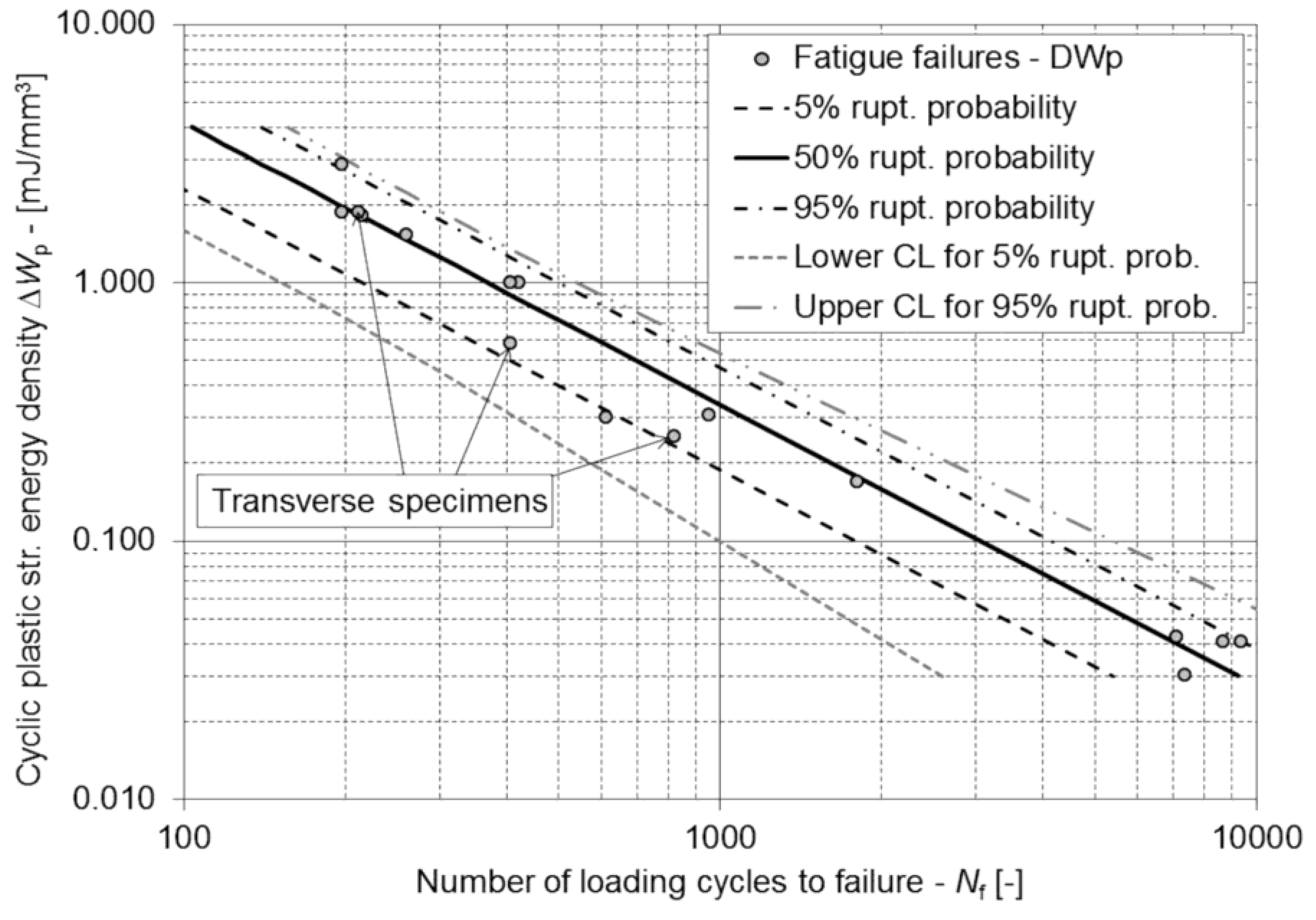
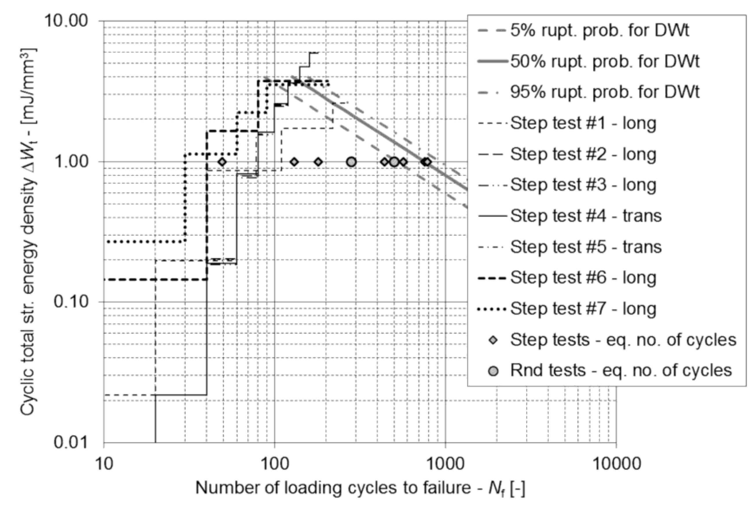
2.3. Modeling the Strain-Energy-Density Fatigue-Life Curve and Its Scatter

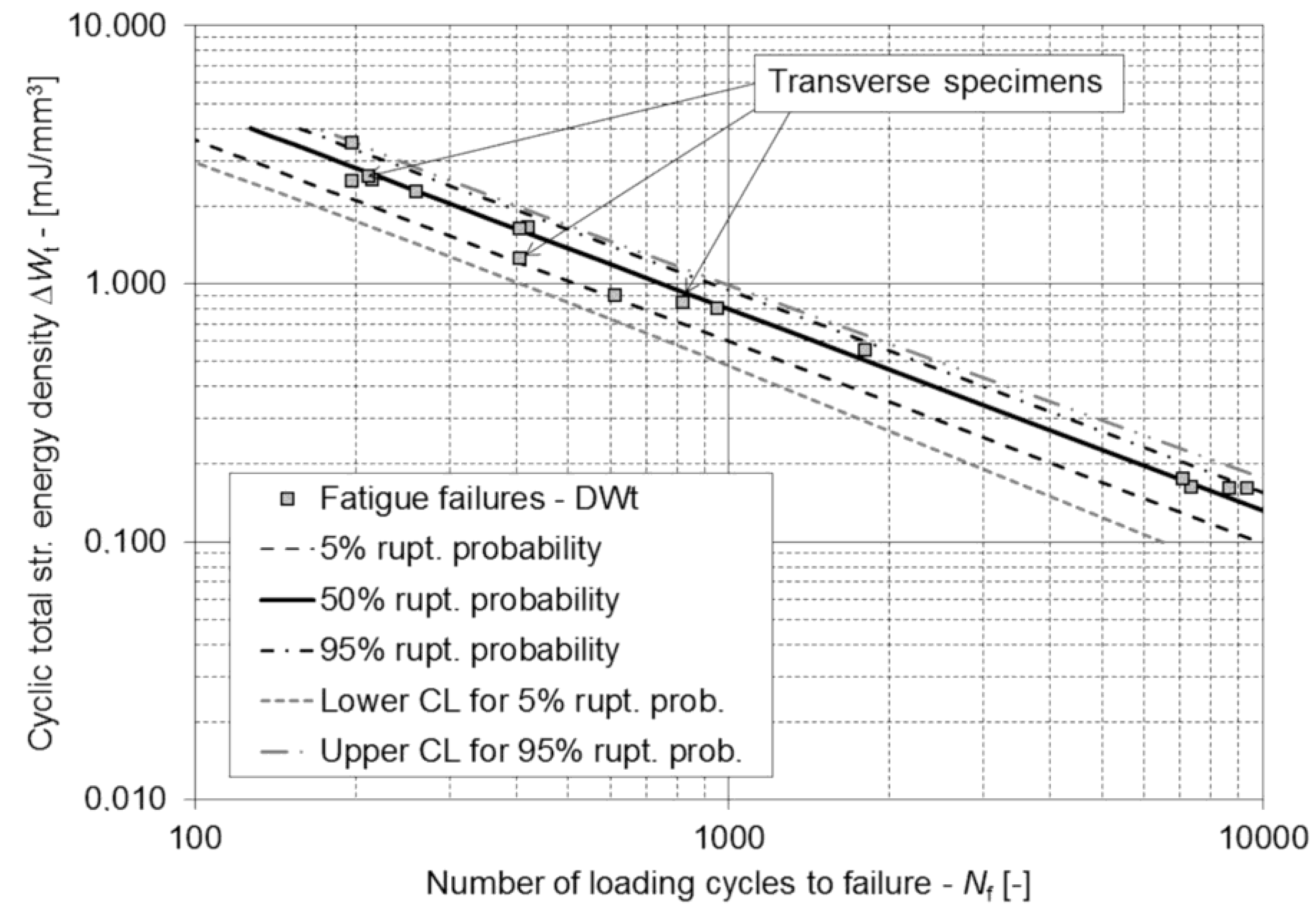
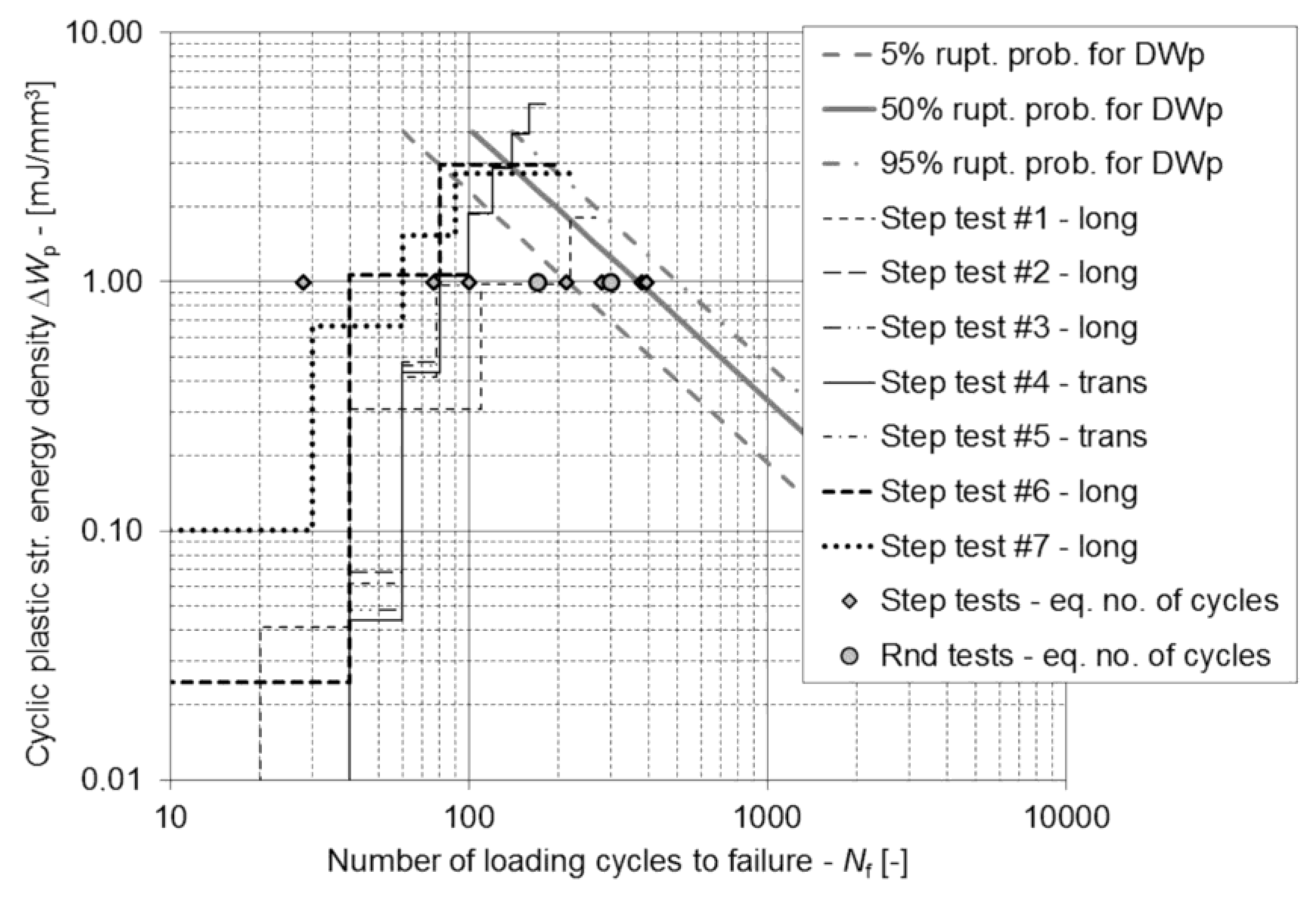
Oftentimes, the researchers perform only constant-amplitude fatigue-life experiments with the specimens from a single production series. To avoid buckling of the specimens the rod-shaped specimens are preferred against the thin flat specimens. Such experimental runs usually result in a good agreement between the proposed fatigue-life models and the experimental data. As opposed to that, our specimens were cut from the 2 mm thick sheet plates from two different production series. Moreover, the specimens were oriented in the longitudinal and transversal directions. Consequently, a higher scatter of experimental results was obtained if compared to, e.g., Park et al. [18]. To model the fatigue life appropriately and to estimate the corresponding confidence intervals the energy fatigue-life curve with its scatter should be determined.

Equations (4) and (5) are another form of the Basquin equation of the S-N curve. In the past we developed a method for modeling the S-N curve and its scatter with a two-parametric Weibull’s probability density function (PDF). The Weibull’s PDF had a constant shape parameter β and the variable scale parameter η with the functional form of the Basquin equation [25,26]. The same approach can be followed to model the energy fatigue-life curves from Equations (4) and (5), together with their scatter. The idea is to model the scatter of the number of loading cycles to failure N_f at an arbitrary strain-energy density level ΔW using the two-parametric Weibull’s PDF:

$$f(N_{\mathrm{f}}|\Delta W)=\frac{\beta }{\eta (\Delta W)}\cdot {\left(\frac{N_{\mathrm{f}}}{\eta (\Delta W)}\right)}^{\beta -1}\cdot \exp \left[-{\left(\frac{N_{\mathrm{f}}}{\eta (\Delta W)}\right)}^{\beta }\right];N_{\mathrm{f}},\beta ,\eta >0$$

(7)

$$\beta =\mathrm{const}.$$

(8)

$$\eta (\Delta W)={10}^{a_0+a_1\cdot \log (\Delta W)}$$

(9)

The scale parameter η(ΔW) represents the number of loading cycles to failure N_f for a 63.2% probability of rupture at the strain-energy level ΔW. Since Equations (4) and (5) can be transformed into the following form:

$$\Delta W\cdot N_{\mathrm{f}}^m=C\to \log (N_{\mathrm{f}})=\frac{\log (C)}{m}-\frac{1}{m}\cdot \log (\Delta W)$$

(10)

The two parameters a₀ and a₁ from Equation (9) are equal to:

$$a_0=\frac{\log (C)}{m};a_1=-\frac{1}{m}$$

(11)

The three parameters a₀, a₁ and β of the above-described model can be determined on the basis of the n constant-amplitude fatigue-life experiments that result in the data set $\left\{\left(\Delta W_i,N_{\mathrm{f},i}\right);i=1,\dots ,n\right\}$. This is achieved by minimizing the logarithmic maximum-likelihood cost function (abbreviation MLE) with the following form [26,27]:

$$MLE\left[a_0,a_1,\beta \right]={\displaystyle \sum _{i=1}^n\left({\delta }_i\cdot \ln \left[f(N_{\mathrm{f},i}|\Delta W_i)\right]+(1-{\delta }_i)\cdot \ln \left[1-F(N_{\mathrm{f},i}|\Delta W_i)\right]\right)}$$

(12)

The MLE function is a compound of the Weibull’s PDF from Equation (7) and its corresponding cumulative distribution function F(N_f,i|ΔW_i):

$$F(N_{\mathrm{f},i}|\Delta W_i)={\displaystyle \underset{0}{\overset{N_{\mathrm{f},i}}{\int }}f(N_{\mathrm{f}}|\Delta W_i)\cdot d{N}_{\mathrm{f}}=}1-\exp \left[-{\left(\frac{N_{\mathrm{f},i}}{\eta (\Delta W_i)}\right)}^{\beta }\right]$$

(13)

The mixing weight in Equation (12) is a δ_i parameter, which is an indicator of the fatigue failure (δ_i = 1). If the fatigue-life experiment was terminated before the fatigue failure occurred, the δ_i parameter is equal to 0.

The MLE function from Equation (12) cannot be minimized analytically. In order to minimize it a numerical minimization procedure should be applied. We used a real-valued genetic algorithm for this purpose and checked the estimated parameters with another minimization algorithm, i.e., a differential ant-stigmergy algorithm. Both algorithms were successfully used before for similar purposes [25,26,27]. The primary choice is the real-valued genetic algorithm, since it is faster (but occasionally less efficient) than the alternative algorithm. In order to obtain reliable estimates of the three parameters a₀, a₁ and β the optimization algorithms should be repeated with various initial conditions. Details of the two algorithms can be found in the literature [25,26].

After the three parameters a₀, a₁ and β are estimated, the number of loading cycles to failure N_f,p can be estimated for the arbitrary strain-energy-density level ΔW and the probability of rupture p as follows:

$$p=F(N_{\mathrm{f},\mathrm{p}}|\Delta W)=1-\exp \left[-{\left(\frac{N_{\mathrm{f},\mathrm{p}}}{\eta (\Delta W)}\right)}^{\beta }\right]\to N_{\mathrm{f},\mathrm{p}}=\eta (\Delta W)\cdot {\left[-\ln (1-p)\right]}^{1/\beta }$$

(14)

In this manner, the fatigue-life curves for an arbitrary probability of rupture p can be constructed.

Due to the relatively small number of constant-amplitude fatigue life tests (n = 16, see Section 2.1) the confidence limits for the modeled fatigue-life curves need to be estimated. Two confidence limits were estimated in our case: i.) a lower α = 5% confidence limit for the fatigue-life curve that corresponds to the p = 5% probability of rupture and ii.) an upper α = 5% confidence limit for the fatigue-life curve that corresponds to the p = 95% probability of rupture. The two confidence limits were estimated using the Monte Carlo method. Following this approach, a thousand simulated fatigue-life data sets of size n = 16 were artificially generated for each of the two fatigue-life curves. The data sets were generated with a random-number generator according to the Weibull’s PDF from Equation (7), with the parameters a₀, a₁ and β that were estimated from the experimentally determined data set. For each artificial data set the three parameters and the corresponding p-probability fatigue-life curve were estimated. From the family of these fatigue-life curves the lower or upper confidence limit was finally calculated for the various strain-energy-density levels ΔW.

3. Results

The results of the constant strain-amplitude experiments are presented in Figure 7 for the dependency between the plastic strain-energy density ΔW_p and the number of loading cycles to failure N_f, and in Figure 8 for the dependency between the total strain-energy density ΔW_t and the number of loading cycles to failure N_f. In both figures there are fatigue-life curves for 5%, 50% and 95% probabilities of survival, together with the 5% confidence lower limit of the 5% fatigue-life curve and the 5% confidence upper limit of the 95% fatigue-life curve. The corresponding parameters C_p/t, m_p/t and β_p/t are presented in

Table 2. Estimated parameters of the strain-energy fatigue-life durability curves.

Parameter	Plastic Strain-Energy Density Model f(Nf |ΔWp)	Total Strain-Energy Density Model f(Nf |ΔWt)
Parameter C for 50% probability of rupture	625.41	176.45
Parameter C for η	679.26	183.83
Parameter m	1.089	0.781
Parameter β	4.833	6.986

. The parameters a₀, a₁ and β from Equations (9–13) were estimated using a real-valued genetic algorithm. It took 10,000 iterations and 10 repetitions of the algorithm for both fatigue-life models (ΔW_p-N_f and ΔW_t-N_f). There were no differences between the parameters that were estimated with the real-valued genetic algorithm and the differential ant-stigmergy algorithms, despite the genetic algorithm being approximately 20% faster for the 10,000 iterations. The governing parameters of the two optimization algorithms were the same as before [26]. The Monte Carlo simulations for estimating the confidence limits were run with the same set-up.

Figure 9a shows the scatter of the stabilized hysteresis for the strain amplitude ε_a = 1.0% from different constant-amplitude and step-strain low-cycle fatigue experiments. Figure 9b shows the evolution of the stabilized hysteresis loops for the step-strain test no. 8. The closed hysteresis loops resulting from one block of the random fatigue-life tests are presented in Figure 10a,b for the two random-load time series. They are shown at half of the fatigue life. The blocks of the random loading in Figure 4 were repeated 29 times, until the failure of the specimen. The blocks of the random loading in Figure 5 were repeated 13 times, until the failure of the specimen.

In Figure 11, the results of the step-strain and the random fatigue-life experiments are compared with the plastic strain-energy-density fatigue-life curve. The design of the step-strain experiments is shown with different lines. After the specimen ruptured the results of the step-strain and random experiments were recalculated for the target equivalent strain-energy-density level ΔW_eq of 1 mJ/mm³ for both studied cases. The equivalent numbers of loading cycles to failure N_f,eq, which were calculated using Equation (6), are marked with diamond marks for the step-strain experiment. The N_f,eq values from the random experiments are marked with circles. In Figure 12, the same results are presented in the same manner for the total strain-energy density fatigue-life curve. In both figures only the results for seven step-strain tests are shown. This is because step-strain test no. 2 did not result in low-cycle fatigue failure, but failed due to buckling along the stronger axis at a strain-amplitude level of 1.75%. This is because only the weaker axis of the specimen is supported with the applied anti-buckling device during the low-cycle fatigue experiments. For this reason, the results of the step-strain test no. 2 were not considered for further data processing.

4. Discussion

It can be concluded from Table 2 that the number of loading cycles to failure is almost directly proportional to the accumulated plastic strain-energy density, because the exponent m_p for the ΔW_p–N_f curve is approximately equal to 1.0. This implies that the predicted number of loading cycles to failure N_f could also be simply calculated on the basis of the accumulated strain-energy density of the tensile test [19,20]. However, this is not so for the case of the total strain-energy density ΔW_t, where the exponent m_t is significantly different from the value of 1.0. On the other hand, the scatter of the results is much smaller for the ΔW_t–N_f fatigue-life curve than for the ΔW_p–N_f fatigue-lie curve—see Figure 7 and Figure 8. The ratio between the fatigue-life curves for the 95% and 5% probability of survival along the N_f axis is only 1.79 for the ΔW_t–N_f fatigue-life curve, whereas it is 2.32 for the ΔW_p–N_f fatigue-life curve. Moreover, the results of the constant strain-amplitude experiments lie on a straight line for the ΔW_t–N_f fatigue-life curve (Figure 8), whereas a slight banana-like cloud of points can be observed in the case of the ΔW_t–N_f fatigue-life curve in Figure 7. From these results, it can be concluded that the total strain-energy fatigue-life curve better represents the constant-amplitude experimental data and that the inverse power law from Equation (4) might not be the correct model for estimating the relationship between the cyclic plastic strain-energy density ΔW_p and the corresponding number of loading cycles to failure N_f. Therefore, in the future, additional constant-amplitude fatigue experiments should be carried out to determine the true shape of the ΔW_p–N_f fatigue-life curve.

Since the scatter of the ΔW_t–N_f fatigue-life curve is significantly smaller than the scatter of the ΔW_p–N_f fatigue-life curve, the corresponding confidence interval is narrower for the W_t–N_f fatigue-life curve. This fact again implies that the ΔW_t–N_f relationship should be used for performing the fatigue-life predictions in practice. Nevertheless, we have calculated the equivalent number of loading cycles to failure N_f,eq at the equivalent strain-energy density level ΔW_eq of 1 mJ/mm³ for both cases of the modeled fatigue-life curves.

From Figure 7 and Figure 8 we can see that the low-cycle fatigue lives for the three transversely oriented specimens lie mostly between the fatigue-life curves for a 5% and 50% probability of survival, which is not the case for the longitudinally oriented specimens. However, this difference between the fatigue lives of the longitudinally and transversely oriented specimens is not statistically significant, because of the small total number of specimens. We can also conclude from Figure 9a that the stabilized hysteresis loop for the transversely oriented specimen lies in the middle of the scattered, stabilized hysteresis loops for the longitudinally oriented specimens. This means that there were no significant differences between the cyclic plastic and elastic strain-energy densities among the differently oriented specimens. From Figure 10 it can be seen that the stabilized envelopes of the loading cycles are very similar for the two random strain histories, despite significantly different random loadings. Such a result was expected with regards to the relatively low scatter of the stabilized, closed hysteresis loops at strain amplitudes higher than 1.0%—see also Figure 9a.

From Figure 9b, it can be concluded that the stabilized hysteresis loops in the step-strain test no. 8 are fully evolved and no peculiarities can be seen. The same effect was also observed for the other step-strain tests, with the exception of step-strain test no. 2, where the failure occurred due to buckling along the stronger axis of the specimen. Stress-hardening effects occurred above strain amplitudes of 0.4%. The maximum stress hardening was around 20% for the strain amplitudes larger than 1.0%. The most significant stress hardening occurred up to 20 loading cycles, thus, this was considered as the minimum number of loading cycles within one block of the step-strain tests, with the exception of the step-strain test no. 2.

In an ideal case, all the calculated equivalent number of loading cycles to failure N_f,eq at the selected equivalent strain-energy density ΔW_eq would be uniformly scattered around the fatigue-life curves for a 50% probability of rupture. It can be seen from Figure 11 and Figure 12 that in both cases at the selected ΔW_eq level four out of nine variable strain-amplitude experiments lie within the 90% scatter band of the fatigue-life curves, which were estimated from the constant strain-amplitude experiments. However, eight out of nine variable strain-amplitude experimental results differed from the average fatigue-life curves at the selected ΔW_eq level by less than a decade. This result is relatively good, because the specimens were prepared from two different production series and the linear damage-accumulation theory was applied to calculate the equivalent number of loading cycles to failure N_f,eq. Besides, the loading-cycle sequence was not considered when calculating the equivalent number of loading cycles to failure N_f,eq for random loads. The only issue related to the presented results is that most of the calculated equivalent fatigue lives (N_f,eq) are not conservative. Most of them lie to the left of the 50% fatigue-life curve, which might lead to a conclusion that the applied damage accumulation method has a limited prediction ability in this case. To prove this, additional step-tests and random tests should be carried out in the future. Furthermore, it can be concluded from Figure 11 and Figure 12 that the random fatigue-life data better suit the fatigue-life energy curves than the step-strain data. The specimen orientation is not a cause for such a discrepancy, because there is one longitudinal and one transversal specimen among the worst two performers. Since all the specimens had approximately the same roughness due to the cutting process and the worst two specimens were cut from the same sheet plate, the cause for such a discrepancy should be related to the material microstructure. Unfortunately, it was not analyzed for these two specimens. From the variable-amplitude experimental results, no significant differences in the fatigue life could be observed between the longitudinal and transversely oriented specimens. There were also no significant differences in the fatigue-life predictions between the plastic- and total strain-energy-density approaches. The final conclusion of the article is that the linear damage-accumulation rule combined with the cyclic strain-energy-density approach is a good starting point for engineering predictions of the fatigue life of the AZ31 magnesium alloy if the fatigue-life curve and its scatter are known.

5. Conclusions

In this article, an approach to predicting the low-cycle fatigue life of the AZ31 magnesium alloy is presented. It is based on modeling the strain-energy fatigue-life curves and their scatter from the results of constant strain-amplitude fatigue experiments. The flat AZ31 specimens were made of sheet metal plates and were tested on a hydraulic test rig. Various load histories were chosen to characterize the behavior of the AZ31 under tensile-compressive, constant-amplitude and variable-amplitude loadings. Fatigue-life curves were modeled for both the cyclic plastic- and total strain-energy densities. The fatigue-life curves that are based on the total cyclic strain-energy density suit the fatigue-life data much better than the curves that were obtained from the cyclic plastic strain-energy densities. The results from the variable-amplitude loading were compared with the modeled fatigue-life curves using the equivalent strain-energy-density approach. From the presented results it can be concluded that the accumulated strain-energy density during cyclic loading can be applied as a relevant engineering durability criterion for estimating fatigue-life of structures from the AZ31 magnesium alloy. However, the well-known drawbacks of the linear damage accumulation rule combined with the uncertainty related to the local microstructure of the half-products should be considered when assessing the accuracy of the predicted fatigue life.

References

1. Klemenc, J.; Seruga, D.; Nagode, M. Plastic and total energy as the basis of durability prediction for magnesium alloy AZ31. In Proceedings of the 27th International Conference on Processing and Fabrication of Advanced Materials (PFAM-XXVII), Jönköping, Sweden, 27–29 May 2019. [Google Scholar]
2. Lukac, P.; Kocich, R.; Greger, M.; Padalka, O.; Szaraz, Z. Microstructure of AZ31 and AZ61 Mg alloys prepared by rolling and ECAP. Kovove Mater. 2007, 45, 115–120. [Google Scholar]
3. Kocich, R.; Kursa, M.; Macháčková, A. FEA of Plastic Flow in AZ63 Alloy during ECAP Process. Acta Phys. Pol. A 2012, 122, 581–587. [Google Scholar] [CrossRef]
4. Smith, K.N.; Watson, P.; Topper, T.H. A stress-strain function for the fatigue of metals. J. Mater. 1970, 5, 767–778. [Google Scholar]
5. Ellyin, F.; Kujawski, D. Plastic strain energy in fatigue failure. J. Press. Vessel Technol. 1984, 106, 342–347. [Google Scholar] [CrossRef]
6. Golos, K.M.; Ellyin, F. A total strain energy density theory for cumulative fatigue damage. J. Press. Vessel. Technol. 1988, 110, 36–41. [Google Scholar] [CrossRef]
7. Golos, K.M. Multiaxial fatigue criterion with mean stress effect. Int. J. Press. Vessel Pip. 1996, 69, 263–266. [Google Scholar] [CrossRef]
8. Koh, S.K. Fatigue damage evaluation of high pressure tube steel using cyclic strain energy density. Int J Press. Vessel Pip. 2002, 79, 791–798. [Google Scholar] [CrossRef]
9. Park, S.H.; Hong, S.G.; Lee, B.H.; Bang, W.; Lee, C.S. Low-cycle fatigue characteristics of rolled Mg-3Al-1Zn alloy. Int. J. Fatigue 2010, 32, 1835–1842. [Google Scholar] [CrossRef]
10. Dallmeier, J.; Huber, O.; Saage, H.; Eigenfeld, K. Uniaxial cyclic deformation and fatigue behavior of AK50 magnesium alloy sheet metals under symmetric and asymmetric loadings. Mater. Des. 2015, 70, 10–30. [Google Scholar] [CrossRef]
11. Lin, Y.C.; Chen, X.M.; Liu, Z.H.; Chen, J. Investigation of uniaxial low-cycle fatigue failure behavior of hot-rolled AZ91 magnesium alloy. Int. J. Fatigue 2013, 48, 122–132. [Google Scholar] [CrossRef]
12. Roostaei, A.; Pahlevanpour, A.; Behravesh, S.B.; Jahed, H. On the definition of elastic strain energy density in fatigue modeling. Int. J. Fatigue 2019, 121, 237–242. [Google Scholar] [CrossRef]
13. Zhu, S.P.; Lei, Q.; Huang, H.Z.; Yang, Y.J.; Peng, W. Mean stress effect correction in strain-energy based fatigue life prediction of metals. Int. J. Damage Mech. 2017, 26, 1219–1241. [Google Scholar] [CrossRef]
14. Jahed, H.; Varvani-Farahani, A.; Noban, M.; Khalaji, I. An energy-based fatigue life assessment model for various metallic materials under proportional and non-proportional loading conditions. Int. J. Fatigue 2007, 29, 647–655. [Google Scholar] [CrossRef]
15. Park, J.; Nelson, D. Evaluation of an energy-based approach and a critical plane approach for predicting constant amplitude multiaxial fatigue life. Int. J. Fatigue 2000, 22, 23–39. [Google Scholar] [CrossRef]
16. Ince, A. A generalized mean stress correction model based on distortional strain energy. Int. J. Fatigue 2017, 104, 273–282. [Google Scholar] [CrossRef]
17. Ince, A. A mean stress correction model for tensile and compressive mean stress fatigue loadings. Fatigue Fract. Eng. Mater. Struct. 2017, 40, 939–948. [Google Scholar] [CrossRef]
18. Park, S.H.; Hong, S.-G.; Lee, B.H.; Lee, C.S. Fatigue life prediction of rolled AZ31 magnesium alloy using an energy-based model. Int. J. Mod. Phys. B 2008, 22, 5503–5508. [Google Scholar] [CrossRef]
19. Letcher, T.; Shen, M.H.H.; Scott-Emuakpor, O.; George, T.; Cross, C. An energy-based critical fatigue life prediction method for Al6061-T6. Fatigue Fract. Eng. Mater. Struct. 2012, 35, 861–870. [Google Scholar] [CrossRef]
20. Ozaltun, H.; Shen, M.H.H.; George, T. An energy based fatigue life prediction framework for in-service structural components. Exp. Mech. 2011, 51, 707–718. [Google Scholar] [CrossRef]
21. Kabir, S.M.H.; Yeo, T. Evaluation of an energy-based fatigue approach considering mean stress effects. J. Mech. Sci. Tech. 2014, 28, 1265–1275. [Google Scholar] [CrossRef]
22. Jahed, H.; Albinmousa, J. Multiaxial behaviour of wrought magnesium alloys – A review and suitability of energy-based fatigue life model. Theor. Appl. Fract. Mech. 2014, 73, 97–108. [Google Scholar] [CrossRef]
23. Wang, C.; Luo, T.J.; Zhou, J.X.; Yang, Y.S. Anisotropic cyclic deformation behaviour of extruded ZA81M magnesium alloy. Int. J. Fatigue 2017, 96, 178–184. [Google Scholar] [CrossRef]
24. Dallmeier, J.; Denk, J.; Huber, O.; Saage, H.; Eigenfeld, K. A phenomenological stress-strain model for wrought magnesium alloys under elastoplastic strain-controlled variable amplitude loading. Int. J. Fatigue 2015, 80, 306–323. [Google Scholar] [CrossRef]
25. Klemenc, J.; Fajdiga, M. Estimating S-N curves and their scatter using a differential ant-stigmergy algorithm. Int. J. Fatigue 2012, 43, 90–97. [Google Scholar] [CrossRef]
26. Klemenc, J. Influence of fatigue–life data modelling on the estimated reliability of a structure subjected to a constant-amplitude loading. Reliab. Eng. Syst. Saf. 2015, 142, 238–247. [Google Scholar] [CrossRef]
27. Klemenc, J.; Fajdiga, M. Joint estimation of E-N curves and their scatter using evolutionary algorithms. Int. J. Fatigue 2013, 56, 42–53. [Google Scholar] [CrossRef]
28. Goodfellow – your global supplier for materials. Available online: https://www.goodfellow.com/catalogue/GFCat2H.php?ewd_token=28skhnCrjhctQ0VRfphfvd6PniE1Vm&n=wFtvXD7C9WyVocNzf9Oip0qnk2dP9i&ewd_urlNo=GFCat2L3&Head=MG01 (accessed on 30 August 2019).
29. Seruga, D.; Nagode, M.; Klemenc, J. Measurement of stress-strain response during cyclic tests. In Proceedings of the 27th International Conference on Processing and Fabrication of Advanced Materials (PFAM-XXVII), Jönköping, Sweden, 27–29 May 2019. [Google Scholar]
30. Seruga, D.; Nagode, M.; Klemenc, J. Eliminating friction between flat specimens and an antibuckling support during cyclic tests using a simple sensor. Meas. Sci. Technol 2019. [Google Scholar] [CrossRef]
Figure 1. Flat specimens for tensile and low-cycle fatigue experiments on the AZ31 alloy; (measurement unit is mm).
Metals 09 00973 g001
Figure 2. Microstructure of the specimens: (a) after tensile loading; (b) after cyclic loading.
Metals 09 00973 g002
Figure 3. Experimental arrangement for the low-cycle fatigue experiments: (a) schematic representation of the anti-buckling device; (b) real experiment.
Metals 09 00973 g003
Figure 4. Strain time series for the first random-loading experiment.
Metals 09 00973 g004
Figure 5. Strain time series for the second random-loading experiment.
Metals 09 00973 g005
Figure 6. Typical elastic-plastic hysteresis loop of the AZ31 magnesium alloy; strain ε [-], stress σ [MPa].
Metals 09 00973 g006
Figure 7. AZ31 fatigue-life curves for the plastic strain-energy density ΔWp.
Metals 09 00973 g007
Figure 8. AZ31 fatigue-life curves for the total strain-energy density ΔWt.
Metals 09 00973 g008
Figure 9. Closed hysteresis loops for the non-random loading: (a) scatter of stabilized hysteresis loops at 1% strain amplitude; (b) evolution of stabilized hysteresis loops for the step-test 8.
Metals 09 00973 g009
Figure 10. Closed hysteresis loops for the random loadings: (a) 16th loading block of the first random loadings; (b) 7th loading block of the second random loadings.
Metals 09 00973 g010
Figure 11. Fatigue-life curves with the variable-amplitude loading results for the plastic strain-energy density ΔWp (DWp); ΔWp,eq = 1 mJ/mm3.
Metals 09 00973 g011
Figure 12. Fatigue-life curves with the variable-amplitude loading results for the total strain-energy density ΔWt (DWt); ΔWt,eq = 1 mJ/mm3.
Metals 09 00973 g012