Understanding Dephosphorization in Basic Oxygen Furnaces (BOFs) Using Data Driven Modeling Techniques

Abstract

Owing to the continuous deterioration in the quality of iron ore and scrap, there is an increasing focus on improving the Basic Oxygen Furnace (BOF) process to utilize lower grade input materials. The present paper discusses dephosphorization in BOF steelmaking from a data science perspective, which thus enables steelmakers to produce medium and low phosphorus steel grades. In the present study, data from two steel mills (Plant I and Plant II) were collected and various statistical methods were employed to analyze the data. While most operators in steel plants use spreadsheet-based techniques and linear regression to analyze data, this paper discusses on the suitability of selecting various statistical methods, and benchmarking tests to analyze such dephosphorization data sets. The data contains a wide range of operating conditions, both low and high phosphorus input loads, different slag basicity’s, different slag chemistries, and different end point temperatures, etc. The predicted phosphorus partition from various statistical models is compared against plant data and verified against previously published research.

1. Introduction

Dephosphorization of steel is critical due to the rising prices (100% rise in past five years) of iron ore, which has resulted in the use of lower grade iron ores [1]. Increased phosphorus (P) content in steel imparts cold shortness and leads to poor ductility, toughness, formability, and embrittlement [2,3]. It has been observed that the primary driving factor for dephosphorization in steelmaking is the iron oxide content of slag, rather than dissolved oxygen in liquid steel for a given slag basicity over different carbon content of steel. (%P)/[%P] represents the slag/steel phosphorus distribution ratio and it is usually found to be scattered around the calculated equilibrium values for the metal/slag reactions involving iron oxide in slag [3,4]. Developing new infrastructure or modifying existing equipment can be financially demanding in order to effectively decrease P content. Therefore, we must look for cost-effective or relatively inexpensive ways to achieve phosphorus partitioning in large scale. In this context, Machine Learning (ML) and Artificial Intelligence (AI) based techniques can be game-changing in the pursuit of efficient process control [5,6,7]. Most of the previous works on dephosphorization employed mathematical modelling and thermodynamics analysis as tools for understanding dephosphorization. However, the underlying randomness (measurable and non-measurable) in the dephosphorization process results in unpredictable variation in slag composition from one heat to another and, hence, provides the motivation for applying stochastic data driven models to predict phosphorus partition.

In the last few decades, numerous attempts were made to predict phosphorus-partitioning by combining regression-based models with thermodynamic principles that assume equilibrium conditions. Here, we summarize the highlights from some of these efforts. During 1940s, Balajiva and co-workers performed experiments while using a small Electric Arc Furnace (EAF). They presented a correlation of equilibrium phosphorus partition ratio with a varied range of slag chemistries and temperatures [8]. In 1953, Turkdogan and Pearson provided an estimate of the equilibrium constant for the reaction 2[P] + 5(O) = P₂O₅ while studying phosphorus partition [9,10]. Healy developed a mathematical relationship based on thermodynamic data that were obtained from phosphorus activity and phosphate free energy in the CaO-P₂O₅ binary system [11]. The same model was found to accurately estimate the phosphorus partition in a CaO-FeO–SiO₂ and CaO-Fe–SiO₂ systems. Thus, it was inferred that thermodynamic data of the binary CaO-P₂O₅ system can be extrapolated to the complex slags in the CaO-Fe–SiO₂ system. The coefficient of P₂O₅ activity was determined not only from experimental data of independent studies of slag/metal reactions, but also from the standard free energy of the formation of hypothetical pure liquid P₂O₅. Furthermore, Suito and Inoue developed yet another mathematical model to analyze the phosphorus partition ratio during steelmaking, following the works of Turkdogan, where the phosphorus partition is defined as $log\left\{\frac{\left(\%P\right)}{\left[\%P\right]{(\%F{e}_{total})}^{2.5}}\right\}$ [12]. Similarly, in 2000, Turkdogan published a comprehensive evaluation of ${\gamma }_{P2O5}$ or slags with various combinations of CaO, FeO, and P₂O₅ concentrations [13]. More recently, in 2017, Drain et al. discussed thoroughly the significance of removing phosphorus in basic oxygen steelmaking by comparing the results from numerous studies over years [14]. Their in-depth analysis was based on the coefficient of determination ($R^2$) that was obtained from many empirical equations to capture phosphorus partition [15]. An emphasis was made on the structure of these empirical relationships that defined the behavior of phosphorus partition. It was concluded that slag constituents, such as Al₂O₃, TiO₂, and V₂O₅, have detrimental effect on phosphorus partition. In a recent paper, Chattopadhyay and Kumar provided modified phosphorus partition relationships that are based on multiple linear regression for data on two steel plants—low slag basicity (low temperature) and high slag basicity (high temperature) [16]. It was inferred that minimizing phosphorus reversal during blowing and after tapping, and decreasing the tapping temperature were found to be significant in improving the P distribution during BOF steelmaking.

Thermodynamic models are an excellent tool to start with; however, such models alone may not accurately predict dephosphorization in BOF shops because of the large variation in iron ore quality, coke composition, etc. The models employ short range ordering techniques and utilize the concepts of slag structure and slag chemistry. Additionally, the models are strongly dependent on the range of experimental data originally used to derive the correlations. In addition, the model development time is very long and expensive. Furthermore, the accuracy of such models could depend on the quality of the ore. Recently, researchers have also tried to explain dephosphorization from a kinetics and transport phenomena-based approach. However, controlled experiments on single droplets and simulated slag samples have their own limitations. On the other hand, empirical models for predicting dephosphorization have several limitations as they are usually efficient for a specific compositional and temperature range. Furthermore, a fundamental weakness of such data-driven empirical models is that most of such models invoked the tenets regression formalism on an ad-hoc basis, and only a few implemented least-square based techniques to estimate the parameters. Moreover, the adequacy and applicability of multiple linear regression model that are critical to the applicability of a linear analysis were often not examined. For example, error-based assumptions of normality and constant variance were not verified, correlations among the variables were not examined, and influential observations were not dealt with. This may potentially lead to inconsistent predictions. Furthermore, adequate justifications were not provided for taking transformation of variables to fit concerned models to data.

While the authors appreciate all of the previous research on dephosphorization from a physical sciences point of view, owing to huge computational power and super low computational costs, it is perhaps timely to also look at dephosphorization from a data science perspective. Interestingly, there is a notion that the use of linear regression and spreadsheet-based techniques is adequate for analyzing BOF process data. However, from a statistical and data science point of view, it is important to look at the quality and type of data, appropriate ways to sort/cluster data, appropriate techniques to analyze data, and so on. One of the purposes of this article is to develop a technique to formulate a step-by-step method for applying regression-based analysis to dephosphorization. Here, we employ different statistical methods to analyze the process data that were collected from two separate steel plants and the end-point predictions are compared with measured data from the plants. The utility and validity of different models are summarized, and the predictions are also vetted and explained from a metallurgical viewpoint. An elaborate data-driven approach is taken to analyze BOF steel-making data and predict phosphorus partition in steel. The model under consideration is a well-known multiple linear regression (MLR) model that assumes that multiple factors, e.g., %CaO, %MgO etc. affect phosphorus partition in steel in a linear and additive way where the error in prediction is normally distributed [15]. Assumptions on error play key roles in MLR model fit. The validity of these assumptions is discussed emphasizing on the applicability of the current model on other data sets as well. On the other hand, the presence of influential observations and outliers in the data may lead to biased estimations and erroneous predictions. Techniques to identify and eliminate these influential observations are also explored. Moreover, corrective measures are suggested when one or more of these assumptions are invalid.

The paper is arranged in the following order. Theory and methodology are discussed in Section 2, highlighting the theoretical model structure and available analyses options. Results, including some exploratory analyses based on Generalized Linear Model (GLM), are discussed in Section 3. Section 4 deals with interpretation and practical implication of our predictive model, as well as comparison of our model with existing data-driven models. Conclusion and future directions are discussed as part of Section 5.

2. Materials and Methods

Phosphorus partitioning in slag during BOF steel making is quantified in terms of the parameter $l_p$. A higher value of $l_p$ indicates lower phosphorus-base impurities in steel. Thus, it is important to develop a robust predictive model to predict $l_p$ based on information that is available from the predictors to account for the underlying randomness in BOF steelmaking. A simple, yet effective data-driven model in this set-up is a regression-based model. A regression model usually takes various forms, depending on the flexibility and generalization of the background assumptions. One of the well-known regression-based models is a multiple linear regression (MLR) model, which assumes the random error (factor which cannot be explained by the predictors) to be normally distributed [15,17]. In this paper, we investigated various aspects of the MLR model for the data discussed above. For the purpose of numerical analysis, the statistical software R 3.4.4 (University of Auckland, Auckland, New Zealand) was used.

2.1. Nature of the Data

The analysis data set contained observations from n = 13,853 heats from plant I and n = 3084 heats from plant II. $l_p=\log \left\{\frac{\left(\%P\right)}{\left[\%P\right]}\right\}$ considered as the response variable where $\left(\%P\right)$ and $\left[\%P\right]$ are the percentages of phosphorus in slag and in steel, respectively. Temperature (Temp), % of Calcium Oxide (CaO), % of Magnesium Oxide (MgO), % of Silicon Dioxide (SiO₂), % of Iron oxide (FeO), % of Manganese Oxide (MnO), % of Aluminium Oxide (Al₂O₃), % of Titanium Dioxide (TiO₂), and % of Vanadium Pentaoxide (V₂O₅) are the other predictors (feature set). For details on compositional data, refer to

Table 1. Descriptive statistics of all variables taken for analysis from plant I and plant II.

Variable	$\mathit{n}$	Mean	SD	Min	Q1	Median	Q3	Max
Plant I
$l_p$	13,853	4.31	0.30	2.50	4.12	4.32	4.51	7.06
Temp	13,853	1648.82	19.14	1500.00	1635.00	1647.00	1660.00	1749.00
CaO	13,853	42.43	3.62	20.00	40.00	42.40	44.90	55.90
MgO	13,853	9.23	1.37	3.75	8.29	9.09	10.00	16.46
SiO2	13,853	12.89	1.74	5.40	11.70	12.80	14.00	23.30
FeO	13,853	18.22	3.53	7.70	15.72	18.10	20.50	36.00
MnO	13,853	4.80	0.70	2.28	4.38	4.82	5.23	11.98
Al2O3	13,853	1.80	0.48	0.59	1.49	1.74	2.04	7.79
TiO2	13,853	1.13	0.28	0.17	0.93	1.08	1.30	2.21
V2O5	13,853	2.13	0.49	0.25	1.84	2.19	2.48	3.95
Plant II
$l_p$	3084	4.63	0.34	2.77	4.44	4.68	4.87	5.64
Temp	3084	1679.10	27.11	1579.00	1661.00	1678.00	1698.00	1777.00
CaO	3084	53.45	2.30	42.33	52.00	53.49	55.02	64.06
MgO	3084	0.99	0.34	0.30	0.76	0.93	1.15	3.18
SiO2	3084	13.52	1.44	8.16	12.54	13.54	14.50	18.74
FeO	3084	19.34	2.06	13.71	17.88	19.19	20.56	29.72
MnO	3084	0.62	0.18	0.24	0.50	0.59	0.71	2.50
Al2O3	3084	0.94	0.25	0.46	0.78	0.93	1.08	4.09

Abbreviations: $n$: sample size, Mean: arithmetic mean, SD: standard deviation, Min: minimum, Q1: 25th percentile, Median: 50th percentile, Q3: 75th percentile, Max: maximum.

.

2.2. Theoretical Model

The primary structure of a regression-based model with one response and $p$ predictors is given by:

$$Y=f(X_1,\dots ,X_p;\mathit{\beta })+ϵ$$

(1)

where $Y$ is the response variable, $X_1$, …, $X_p$ are $p$ predictors, $f$ is an approximate mathematical function that relates Y with $X_1$, …, $X_p$, $\mathit{\beta }$ is the parameter vector that characterizes the model and $ϵ$ is the random error which cannot be modeled while using $f$. Provided Y is a continuous variable, one of the most basic and relatable choices of $f$ is additive linear function with linearity assumption being imposed on $\mathit{\beta }$, i.e.,

$$Y={\beta }_0+{\beta }_1{X}_1+\dots +{\beta }_p{X}_p+ϵ$$

(2)

where $\mathit{\beta }$ = (${\beta }_0,{\beta }_1,\dots ,{\beta }_p)\prime$. The model in equation (2) is known as MLR model if the error term $ϵ$ has a normal distribution with 0 mean, constant variance (heteroscedasticity), and being stochastically independently distributed. The unknown regression coefficients are estimated by the least squares method [15,17].

Although, it is simple to fit MLR model to a data with continuous response variable, the appropriateness of fitting the model needs to be validated, which otherwise may not provide accurate predictions. Model fitting in regression assumes an approximate full model (with all available predictors) and followed by checking for adequacy of the model, e.g., the validity of assumptions on error structure, correlated covariates, influential observations, outliers and redundant variables, and correspondingly coming up with corrective measures.

2.3. Model Adequacy

The theory behind the MLR model assumes the following: normality of errors, zero mean of the errors, constant variance of the errors, and independence of the errors. For an MLR model to work best on a given data, these assumptions need to be verified. Furthermore, the presence of influential observations (observations with high impact on prediction) also could make predictions inaccurate and should therefore be dealt with. Another serious problem that affects the parameter estimates is multicollinearity, which arises when there is near-linear dependence among the predictors [15,17]. As a result, the standard errors of the model parameter estimates become large, thereby leading to imprecision in the predicted response values. Lastly, an optimized set of predictors need to be selected, which would be sufficient for predicting $l_p$, but would be free from redundant information.

In this work, the normality of errors was verified while using the Normal-Quantile plot (QQ plot) and Shapiro–Wilk’s test [15,17,18]. The validity of assumptions such as linearity of the model and heteroscedasticity were carried out using standardized residual plot graphically [15,17]. The independence of the errors was validated while using Index Plot of the standardized residuals [15,17]. Influential observations, which drastically change the model fit, were detected by implementing Welsch and Kuh Measure (DFFITS) [17,19]. The predictors responsible for multicollinearity were identified while using the Variance Inflation Factor (VIF) [15,17]. Redundant predictors, which did not significantly improve the fit, were eliminated while using the Variable selection procedure of Stepwise Regression [15,17]. The algorithm stopped when the addition of a predictor to the model did not result in a significant reduction of the Akaike Information Criterion (AIC) value [15,17,20]. Finally, corrective measures were undertaken, such as appropriate transformation of response and predictor variables, use of polynomial regression model if linearity did not hold and generalized linear model (GLM), if the normality of errors did not hold [21].

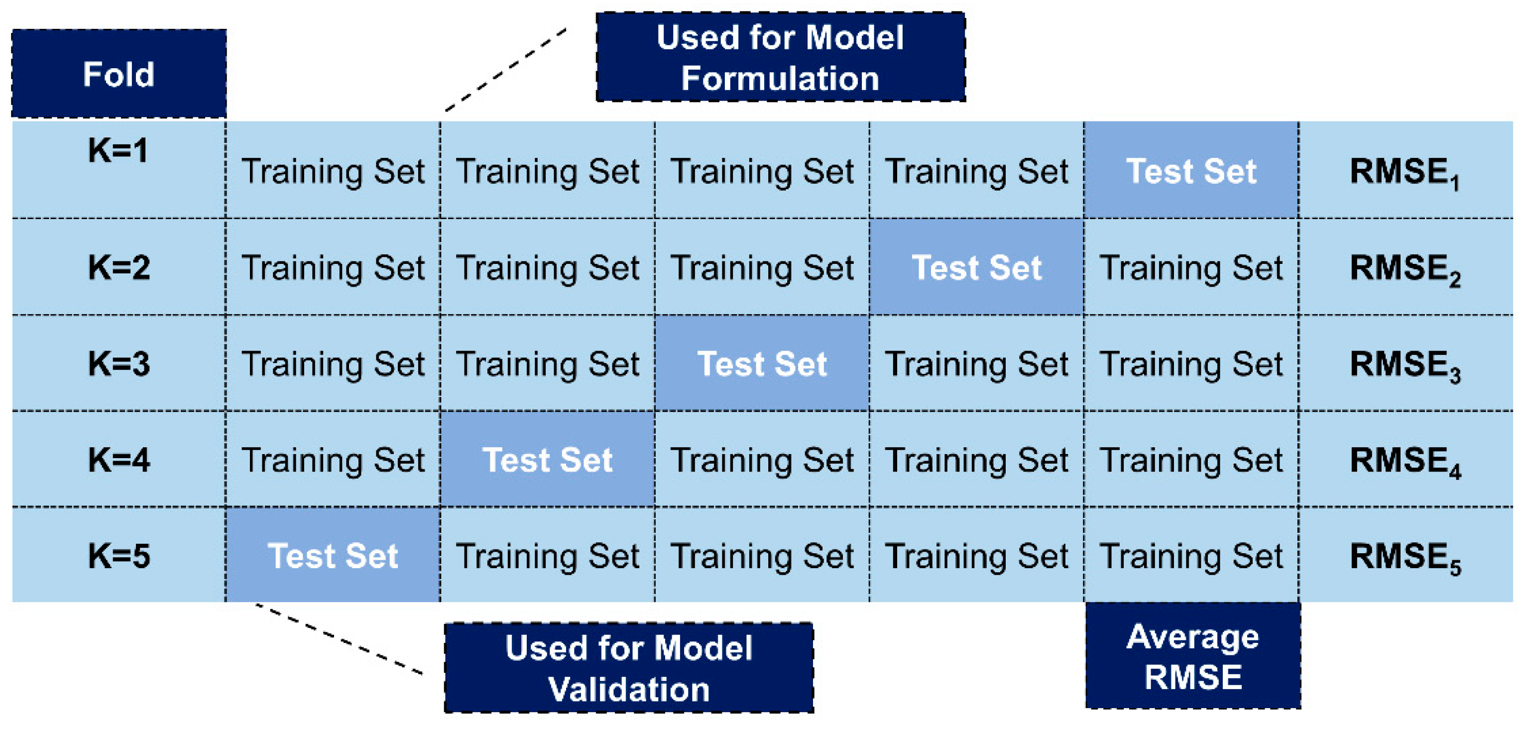
2.4. Model Validation

The K-fold cross validation technique was adopted to check how well the model performed, in general, on test data [22]. The steps used in this work are as follows:

Step 1: The available data set was divided into K-parts with equal or unequal numbers of observations in each. Let these parts be denoted by $P_1,P_2,\dots ,P_{\mathrm{K}}$ and the entire data by $D=\left\{P_1,P_2,\dots ,P_{\mathrm{K}}\right\}.$

Step 2: For any specific $j$, model M was fitted to the part $D\backslash P_j$ (part of $D$ by removing $P_j$) and

$$E_j={\displaystyle \sum }_i{(l_{p,ij}-{\widehat{l}}_{p,ij})}^2$$

(3)

was calculated, where $l_{p,ij}$ is the $i$-th observed value of $l_p$ and ${\widehat{l}}_{p,ij}$ was the $i$-th fitted or predicted value of $l_p$ for the $j$-th iteration.

Step 3: Step 2 was repeated for $j=1,2,\dots ,\mathrm{K}$ and the values of $E_1,E_2,\dots ,E_{\mathrm{K}}$ were calculated.

Step 4: The quantity $E=\sqrt{\frac{1}{\mathrm{K}}{\displaystyle \sum }_{j=1}^{\mathrm{K}}{E}_j}$ was computed which is the root mean squared error (RMSE) over K-folds. Small values of $E$ indicate that the model M has performed reasonably well on other data of similar type.

A flowchart is presented in Figure 1 to summarize steps 1 to 4, as mentioned above.

3. Results

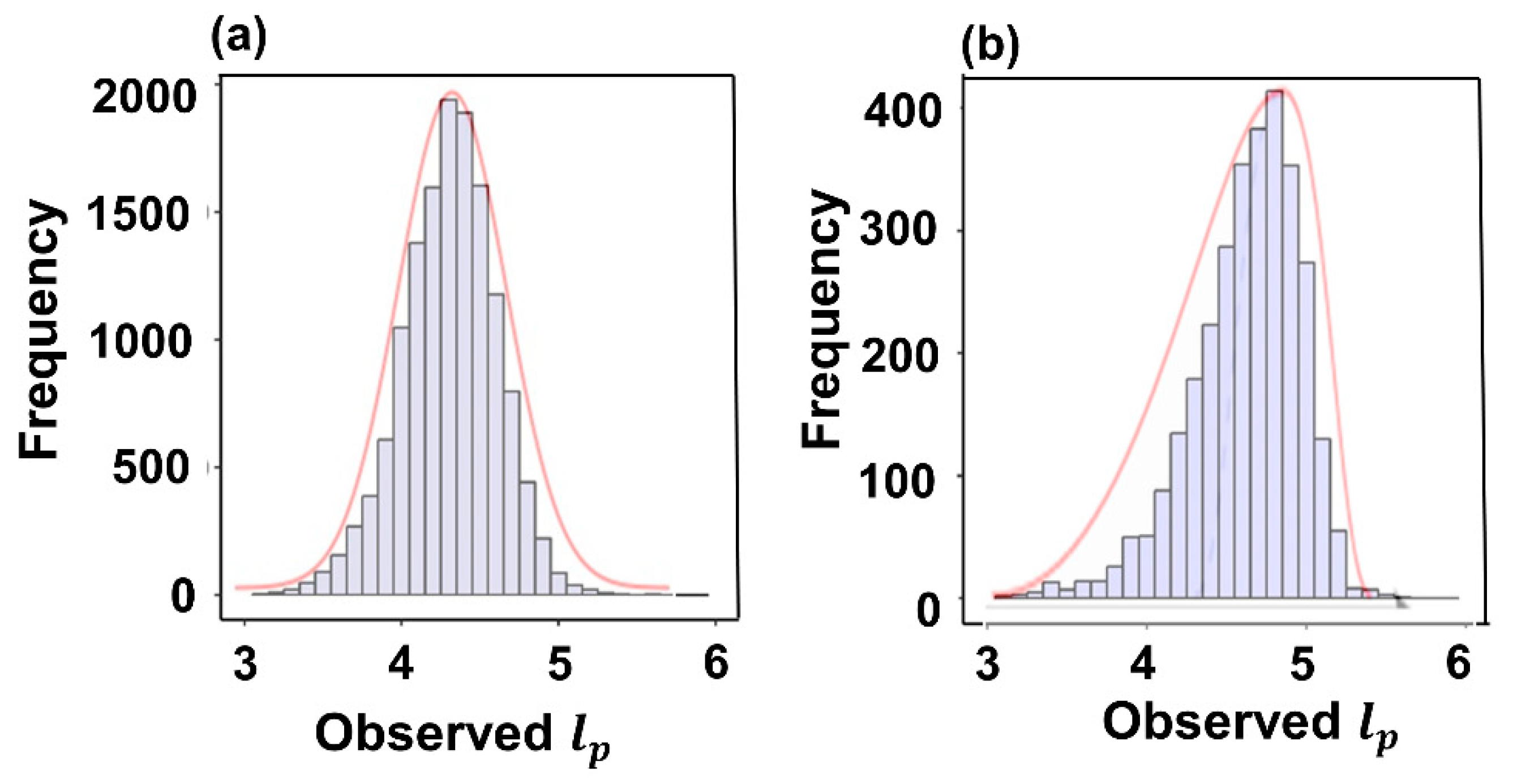
3.1. Descriptive Statistics

Table 1 presents sample size (n), mean (Mean), standard deviation (SD), minimum (Min), first quartile (Q1), median (Median), third quartile (Q3), and maximum (Max) for all variables, both predictors and response. From Table 1, a striking difference in the mean compositions of CaO, MgO and MnO was observed. $l_p$ values were found to have a mean of 4.31 for plant I while for plant II it was 4.73. This indicates that the phosphorus partitioning was more effective in plant II than plant I. Histograms of $l_p$ values were also plotted and they are presented in Figure 2. It can be seen that for plant I, the figure approximately follows a bell-shaped symmetric curve, therefore, indicates the potential normality of errors. However, $l_p$ values for plant II are slightly left skewed, suggesting that there might be an apparent departure from normality. Moreover, the tail probabilities in the histogram seem large, which also indicate evidence against normality.

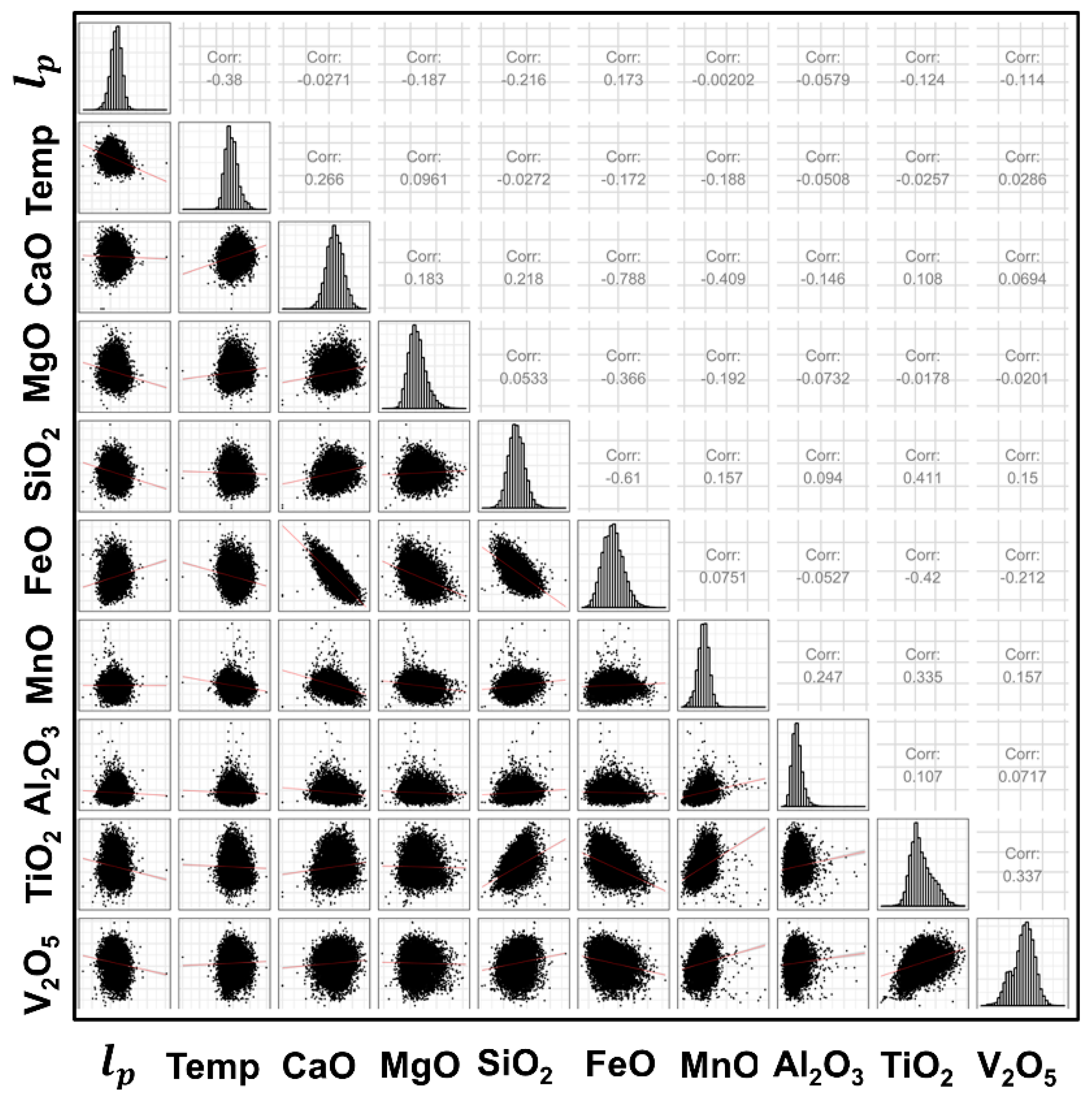
3.2. Individual Predictor Analysis

Simple Linear Regressions (SLRs) were fitted for $l_p$ as the response variable and only one predictor variable at a time. It was found that all predictors except MnO for plant I and Al₂O₃ for plant II were significant individually at 5% level (

Table 2. Parameter Estimates, Standard Errors, T-values, and p-values of the regression parameter estimates.

Plant I	Estimate	Standard Error	T	p
Intercept	15.3238	0.2542	60.28	<0.0001
CaO	0.0209	0.0018	11.64	<0.0001
MgO	−0.0363	0.0022	−16.29	<0.0001
SiO2	−0.0434	0.0022	−19.96	<0.0001
FeO	0.0049	0.0023	2.10	0.0360
MnO	0.0273	0.0042	6.52	<0.0003
Al2O3	−0.0294	0.005	−5.85	<0.0002
TiO2	−0.0573	0.0102	−5.62	<0.0001
V2O5	−0.0299	0.0047	−6.35	<0.0000
Temp	−0.0067	0.0001	−56.71	<0.0001
Plant II	Estimate	Standard Error	T	p
Intercept	19.0145	0.7214	26.40	<0.0001
CaO	0.0019	0.0072	0.26	0.7920
MgO	−0.0382	0.0181	−2.10	0.0350
SiO2	−0.0399	0.0078	−5.10	<0.0001
FeO	−0.0173	0.0097	−1.77	0.0780
MnO	−0.1654	0.0315	−5.24	<0.0001
Temp	−0.0080	0.0001	−44.50	<0.0001

). This indicates that all the predictors or factors effect phosphorus partitioning linearly and individually. The 5% level of significance illustrates the fact that our inference may be wrong 5% of the times on average. A Scatter Plot Matrix is presented in Figure 3 to shed light on the nature and degree of linear relationship between any two variables for plant I.

A similar Scatter Plot Matrix for plant II is not provided in the paper to maintain brevity. Some of the predictors, e.g., Temp, CaO and MgO, were found to have high correlations with $l_p$, which suggests these could potentially be most important factors to predict $l_p$. The adequacy of regression models is generally measured while using a quantity known as $R^2$, which is defined as

$$R^2=1-\frac{SSE}{SST}$$

(4)

where $SSE={\displaystyle \sum }_{i=1}^n{(l_{p,i}-{\widehat{l}}_{p,i})}^2$, $SST={\displaystyle \sum }_{i=1}^n{(l_{p,i}-{\overline{l}}_p)}^2$, and $l_{p,i}$, ${\widehat{l}}_{p,i}$, and ${\overline{l}}_p$ are $i$-th observed value, $i$-th predicted value and sample mean of $l_p$, respectively.

The $R^2$ value does not seem to be too high for any predictor individually, signifying none of them alone can explain the variability in $l_p$ satisfactorily. Furthermore, there does not seem to be a non-linear (polynomial, exponential, or logarithmic) relationship amongst $l_p$ and any other predictor individually.

3.3. Multiple Linear Regression Model Fit

A full MLR model was fit to the data with $l_p$ as the response variable for both plant I and II considering all available predictors. However, this model is not the final one that we would be used for prediction. To come up with the best MLR model, the following steps were carried out.

Identification of influential observations and Outliers: For plant I, 387 influential observations were removed from the analysis data set whose DFFITS values were greater than the cut-off value $2\sqrt{\left(p+1\right)/\left(n-p-1\right)}=0.0537$ [17]. For plant II, cut-off value was taken as $0.1140$ for DFFITS and 22 influential observations were removed from the analysis data set.

Validation of error assumptions: As discussed in Section 2.3, the QQ plot was used to check for normality of errors [17]. QQ plot is a scatter plot between theoretical normal distribution quantiles (percentiles) and quantiles obtained from the observed errors [15]. If the errors are truly normal, then this plot would show points lying on a straight line. QQ plots (Figure 4) of the $l_p$ values did not show adherence to normality for both plant I and II, as the graphs show significant departure from linearity. The Standardized Residual Plots (Figure 5) for plant I and plant II data show almost randomly scattered points without any recognizable pattern, which implies linearity and homoscedasticity assumptions of errors [15]. Index Plot of Standardized Residuals (Figure 6) indicate independence among errors, since the lines joining points frequently crosses the line $x=0$ at regular intervals.

Check for multicollinearity:

Table 3. Variance Inflation Factor (VIF) values corresponding to Predictors used to model data from plant I and plant II.

Plant	Temperature	CaO	MgO	SiO2	FeO	MnO	Al2O3	TiO2	V2O5
Plant I	1.09	8.91	1.97	3.03	14.4	1.83	1.2	1.73	1.16
Plant II	1.06	13.14	1.64	5.7	19.51	1.36	1.52	-	-

presents the VIF values for the predictors considered in plant I and plant II. While using a threshold value of 10, it was observed that the predictor FeO (% of iron oxide in slag) has a strong correlation with other factors for both plant I and II, and CaO has a strong correlation with other factors only for plant II [17]. Generally, multicollinearity generally creates problems of unstable parameter estimates and large standard errors when VIFs are significantly large (in hundreds). Since none of the VIFs were significantly large, and FeO had a huge practical significance in prediction of the phosphorus partition, all of the predictors were kept in the model. On applying stepwise regression, it was observed that none of the features in the model for plant I were redundant. For the data from plant II, the stepwise regression algorithm eliminated CaO and Al₂O₃ based on AIC, as discussed in Section 3. Removing CaO and Al₂O₃ did not significantly change AIC. However, since CaO is practically significant in eliminating phosphorus content from slag, it was kept in the model.

Table 4. Residual Deviances and Akaike Information Criterion (AIC) values corresponding to the redundant Predictors for plant II.

Predictor	Residual Deviance	AIC
Full Model	210.9133	−8176.002
Except CaO	210.9137	−8177.997
Except Al2O3	211.0168	−8178.501

presents Residual Deviances and AIC values for the redundant predictors. It can be seen that the AIC values did not change significantly on removing CaO or Al₂O₃ from the model.

3.4. Final Predictive Models

After removing the influential observations, outliers, and redundant variables, the respective final predictive multiple linear regression models for the plant I and plant II were found to be,

$$\begin{array}{c}\widehat{l_p}=15.324+0.021\left(\%\mathrm{CaO}\right)-0.036\left(\%\mathrm{MgO}\right)-0.043\left({\%\mathrm{SiO}}_2\right)+0.004\left(\%\mathrm{FeO}\right)\\ +0.027\left(\%\mathrm{MnO}\right)-0.029\left(\%{\mathrm{Al}}_2{\mathrm{O}}_3\right)-0.057\left(\%{\mathrm{TiO}}_2\right)\\ -0.029\left(\%{\mathrm{V}}_2{\mathrm{O}}_5\right)-0.006\left(\mathrm{Temp}\right)\end{array}$$

(5)

$$\begin{array}{c}\widehat{l_p}=19.014+0.002\left(\%\mathrm{CaO}\right)-0.038\left(\%\mathrm{MgO}\right)-0.039\left({\%\mathrm{SiO}}_2\right)-0.017\left(\%\mathrm{FeO}\right)\\ -0.165\left(\%\mathrm{MnO}\right)-0.008\left(\mathrm{Temp}\right)\end{array}$$

(6)

The estimates of the least squared regression coefficients, their standard errors, and corresponding t-values for testing if the predictors are significant and the corresponding p-values are presented in Table 2. From the output of plant I, it can be observed that each predictor individually is significant at the 5% level in predicting $l_p.$ The full models are also significant in prediction of $l_p.$ However, the results for plant II show CaO and FeO are not individually significant at the 5% level. The coefficients corresponding to these non-significant predictors should not be used for interpretations.

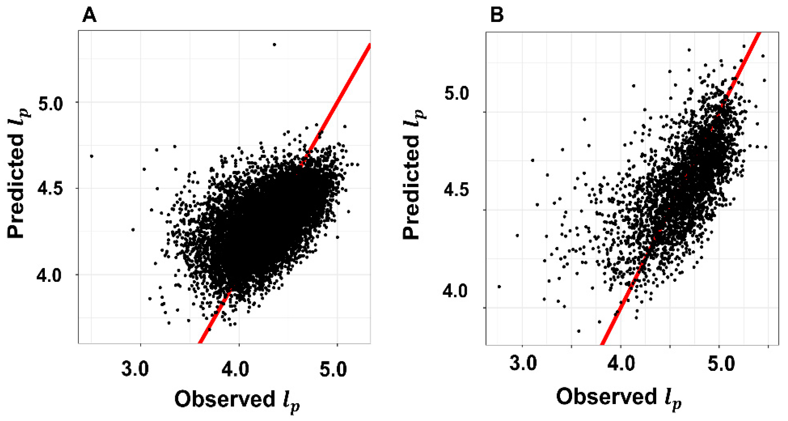
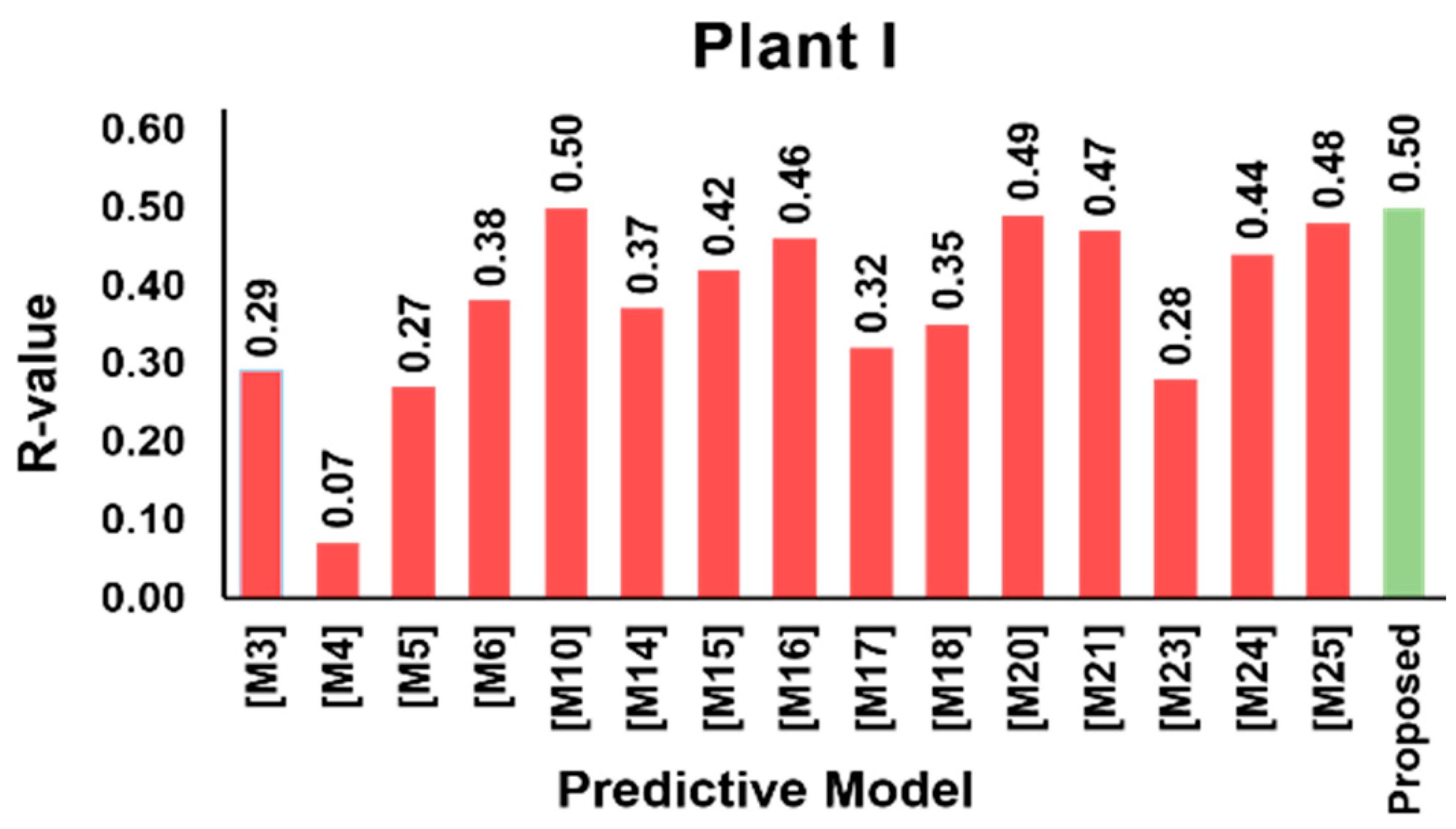
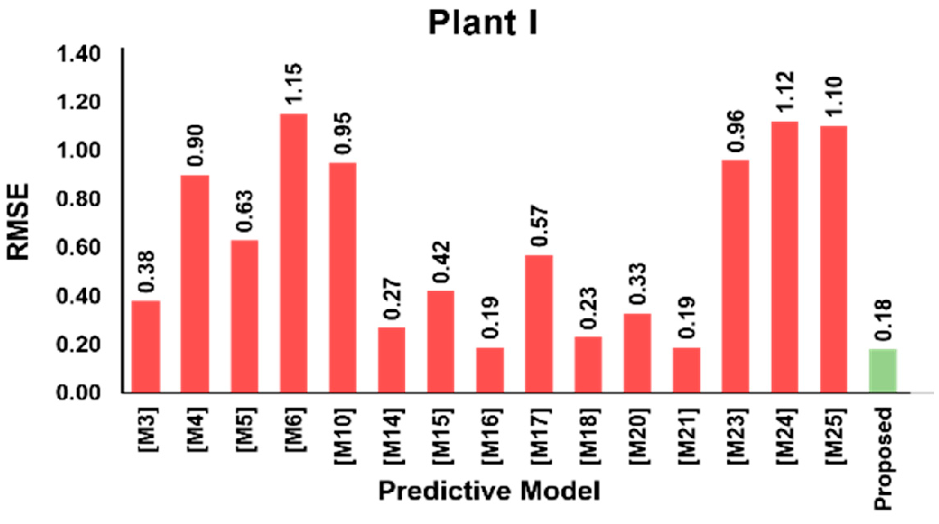
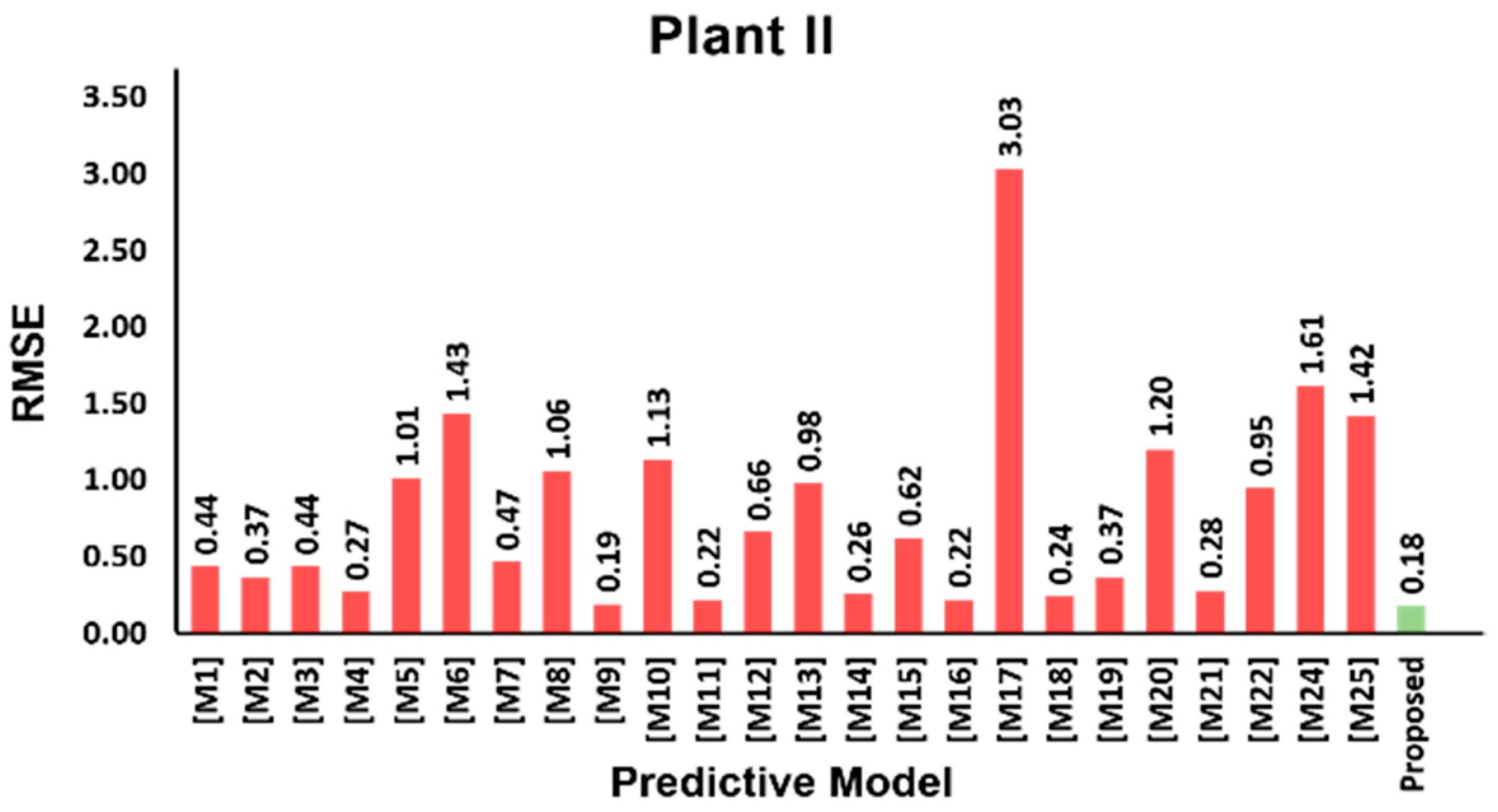
3.5. Model Validation Results

Applying K-fold cross validations with K=10 on the data revealed the root mean squared error ($E$) as 0.262 for plant I and 0.264 for plant II. These relatively small values of $E$ imply that these predictive models perform reasonably well on independent data sets. Figure 7 presents plots of observed or measured values of $l_p$ versus the predicted values of $l_p$. The proximity to the line $y=x$ represents the adequacy of our models in predicting or explaining $l_p$ values.

3.6. Exploratory Analysis

Generalized Linear Model (GLM): When the normality or homoscedasticity (constant variance) of error assumptions get violated in MLR model, we may resort to GLM [21] Although GLM is similar to MLR, the errors are not considered to be normally distributed or may have variances varying with the feature set. Mathematically, we define GLM as $\text{µ}=g^{-1}(X^T\beta ),$ where µ is the theoretical mean of the distribution of the response variable, X is the feature matrix, β is the parameter vector that we want to estimate and $g(.)$ is known as the link function that linearly connects the mean of $Y$ to $X$. Since the response variable $l_p$ here is continuous, we have fewer choices for the family of distributions for the error and the link functions for linking the mean of $Y$ to the feature set X.

Table 5. AIC values for candidate models.

Data	Family of Distribution of Errors	Link Function	AIC
Plant I	Gaussian	“Identity”	2228.1
	Gamma	“Inverse”	2485.7
	Inverse Gaussian	“$1/{\mu }^2$”	2693.5
Plant II	Gaussian	“Identity”	608.6
	Gamma	“Inverse”	893.8
	Inverse Gaussian	“$1/{\mu }^2$”	1067.1

presents details of fitting GLM to the data with the family of error distributions as Gaussian, Gamma, and Inverse Gaussian. The selection criterion for appropriate model is AIC. Note that, the link function as “Identity” for Gaussian error distribution is equivalent to MLR model, as defined in (2). The model with the minimum values of AIC should be selected for prediction. Consequently, for both plants, Gaussian model with “Identity” link provides the minimum AIC values. This further illustrates that an MLR model is more adequate in explaining the variability in $l_p$ than any other candidate linear models and no interaction.

4. Discussion

The predictive models in Equations (5) and (6) provide insights into the nature of the dephosphorization process. Figure 8 and Figure 9 graphically represent the positives and negatives of slag chemistry on P-partitioning in the form of a waterfall plot. The plots suggest that, by tweaking the percentages of the slag components by certain specified degree, it is possible to widen the partition of phosphorus content in slag and steel by a significant amount, which signifies that a lesser amount of phosphorus would be present in steel. For plant I, it was observed that, by increasing the contents of CaO and MnO by 1%, the respective values of $l_p$ can be increased by 0.021%, 0.027% when all other components are kept at fixed levels. These results are in excellent agreement with the findings of Suito et al. [12], wherein it was reported that reducing %MnO in the slag increases $l_p$ value. Furthermore, in slag, Fe resides as FeO and serves two purposes: (a) provides an oxidizing environment (for P to convert to P₂O₅), which promotes dephosphorization, and (b) reduces the basicity of slag by replacing %CaO leading to a deterioration in $l_p$. A rule of thumb for the optimum value of FeO in slag is 15–20 wt%. We observe both effects in Figure 8 and Figure 9. For example, in plant I, where %FeO is smaller than plant II (Table 1), a 1% increase in %FeO improves $l_p$ by 0.005%, probably by promoting the following reaction:${2\mathrm{P}+5\mathrm{FeO}=\mathrm{P}}_2{\mathrm{O}}_5+5\mathrm{Fe}$. However, in plant II, wherein %FeO is larger (i.e., 19.34%) a 1% decrease in %FeO results in a 0.017% increase in $l_p$, which was probably due to a reduction in slag basicity, as discussed above.

On the other hand, a decrease in the contents of MgO, SiO₂, Al₂O₃, TiO₂, V₂O₅, and tapping temperature of the slag by 1%, the respective values of $l_p$ would increase by 0.036%, 0.043%, 0.029%, 0.057%, 0.029%, and 0.006%. A reduction in SiO₂ content of the slag leads to an increase in slag basicity that can improve $l_p$ by promoting the conversion of P to P₂O₅. Similarly, an increase in the MgO content of slag causes an elevation in its viscosity and melting point, deteriorating P-partitioning due to less dynamic interactions. G. Chen et al. [23] reported that, for slags with %FeO more than 24%, $l_p$ reduces with increasing MgO content. Drain et al. [14] had observed that there exists a negative correlation between these metal oxides and $l_p$, which agrees well with the predictions for Al₂O₃, TiO₂, and V₂O₅, as shown in Figure 8.

While using the predictive formulae in (5) and (6), one can determine the extent of dephosphorization on basis of slag chemistry and tapping temperature. Hence, the performance in a plant can be tuned for a new heat by controlling both the slag chemistry and tapping temperature. %FeO in slag needs to be optimized for maximum dephosphorization. This is also related to the yield of steel in a BOF. FeO content beyond the optimum value can lead to a reduction in dephosphorization as well as hot metal to liquid steel yield. Therefore, one can decide on the optimized value of %FeO while using Equations (5) and (6). Furthermore, it was found that SiO₂ and Al₂O₃ have a negative impact on dephosphorization as these compounds reduce the basicity of slag. Basicity can be increased while using CaO, but the effect of CaO on $l_p$ is comparatively less. The marginal effect of adding CaO on $l_p$ is lower than the marginal effect of reducing SiO₂ and Al₂O₃. Hence, the reduction in amount of SiO₂ and Al₂O₃ is more beneficial for dephosphorization and one can decide on the beneficiation technique for reducing these oxides in iron ore. V₂O₅ and TiO₂ contents can also be controlled by proper scrap and iron ore selection. Low V and Ti scrap will be useful for high $l_p$ values.

As discussed in Section 1, there have been few well-established data driven regression models that attempted to predict phosphorus partition measure $l_p$. Depending on the availability of data on the features, 25 existing working models were selected to compare our models with, as described by Equations (5) and (6). These 25 models are given in

Table 6. List of existing candidate model to predict dephosphorization in steel.

Model	Equation
[M1] [24,25]	$\begin{array}{c}\widehat{l_p}=0.06\left[\left(\%\mathrm{CaO}\right)+0.37\left(\%\mathrm{MgO}\right)+4.65\left({\%\mathrm{P}}_2{\mathrm{O}}_5\right)-0.05\left({\%\mathrm{Al}}_2{\mathrm{O}}_3\right)-0.2\left({\%\mathrm{SiO}}_2\right)\right]\\ -10.52+2.5\log \left(\%\mathrm{Fe}.\mathrm{total}\right)+\frac{11570}{\mathrm{Temp}}\end{array}$
[M2] [24,25]	$\begin{array}{c}\widehat{l_p}=0.0680\left[\left(\%\mathrm{CaO}\right)+0.42\left(\%\mathrm{MgO}\right)+1.16\left({\%\mathrm{P}}_2{\mathrm{O}}_5\right)+0.2\left(\%\mathrm{MnO}\right)\right]+\frac{11570}{\mathrm{Temp}}-10.52\\ +2.5\log \left(\%\mathrm{Fe}.\mathrm{total}\right)\end{array}$
[M3] [16]	$\begin{array}{c}\widehat{l_p}=0.07\left(\%\mathrm{CaO}\right)+0.031\left(\%\mathrm{MgO}\right)+0.31\left({\%\mathrm{Al}}_2{\mathrm{O}}_3\right)+0.02\left(\%\mathrm{MnO}\right)+\frac{10911}{\mathrm{Temp}}-11.4\\ +2.84\log \left(\%\mathrm{Fe}.\mathrm{total}\right)\end{array}$
[M4] [16]	$\begin{array}{c}\widehat{l_p}=0.026\left(\%\mathrm{CaO}\right)+0.092\left(\%\mathrm{MgO}\right)+0.08\left({\%\mathrm{Al}}_2{\mathrm{O}}_3\right)+0.04\left(\%\mathrm{MnO}\right)+\frac{12217}{\mathrm{Temp}}-6.29\\ +0.35\log \left(\%\mathrm{Fe}.\mathrm{total}\right)\end{array}$
[M5] [16]	$\begin{array}{c}\widehat{l_p}=0.075\left(\%\mathrm{CaO}\right)+0.025\left(\%\mathrm{MgO}\right)+0.3\left({\%\mathrm{Al}}_2{\mathrm{O}}_3\right)+0.14\left(\%\mathrm{MnO}\right)+\frac{6042}{\mathrm{Temp}}-10.27\\ +3.5\log \left(\%\mathrm{Fe}.\mathrm{total}\right)\end{array}$
[M6] [4]	$\begin{array}{c}\widehat{l_p}=0.431\left[\left(\%\mathrm{CaO}\right)/\left({\%\mathrm{SiO}}_2\right)\right]-0.361\log \left(\%\mathrm{MgO}\right)+\frac{13590}{\mathrm{Temp}}-5.71\\ +0.384\log \left(\%\mathrm{Fe}.\mathrm{total}\right)\end{array}$
[M7] [26]	$\begin{array}{c}\widehat{l_p}=0.072\left[\left(\%\mathrm{CaO}\right)+0.15\left(\%\mathrm{MgO}\right)+0.6\left({\%\mathrm{P}}_2{\mathrm{O}}_5\right)+0.6\left(\%\mathrm{MnO}\right)\right]+\frac{11570}{\mathrm{Temp}}-10.50\\ +2.5\log \left(\%\mathrm{Fe}.\mathrm{total}\right)\end{array}$
[M8] [27]	$\begin{array}{c}\widehat{l_p}=5.89\log \left(\%\mathrm{CaO}\right)+0.5\log \left({\%\mathrm{P}}_2{\mathrm{O}}_5\right)+0.6\left(\%\mathrm{MnO}\right)+\frac{15340}{\mathrm{Temp}}-18.542\\ +2.5\log \left(\%\mathrm{Fe}.\mathrm{total}\right)\end{array}$
[M9] [28]	$\widehat{l_p}=0.056\log \left(\%\mathrm{CaO}\right)+0.5\log \left({\%\mathrm{P}}_2{\mathrm{O}}_5\right)+\frac{12000}{\mathrm{Temp}}-10.42+2.5\log \left(\%\mathrm{Fe}.\mathrm{total}\right)$
[M10] [29]	$\widehat{l_p}=5.6\log \left(\%\mathrm{CaO}\right)+\frac{22350}{\mathrm{Temp}}-21.876+2.5\log \left(\%\mathrm{Fe}.\mathrm{total}\right)$
[M11] [9,30]	$\widehat{l_p}=0.5\log \left({\%\mathrm{P}}_2{\mathrm{O}}_5\right)+\frac{12625}{\mathrm{Temp}}-7.787+2.5\log \left(\%\mathrm{Fe}.\mathrm{total}\right)$
[M12] [8,31,32]	$\widehat{l_p}=5.9\log \left(\%\mathrm{CaO}\right)+0.5\log \left({\%\mathrm{P}}_2{\mathrm{O}}_5\right)-0.00461\mathrm{Temp}-2.0845+2.5\log \left(\%\mathrm{Fe}.\mathrm{total}\right)$
[M13] [8,31,32]	$\widehat{l_p}=5.39\log \left(\%\mathrm{CaO}\right)+0.5\log \left({\%\mathrm{P}}_2{\mathrm{O}}_5\right)-0.00447\mathrm{Temp}-3.0355+2.5\log \left(\%\mathrm{Fe}.\mathrm{total}\right)$
[M14] [4]	$\begin{array}{c}\widehat{l_p}=0.346\left[\left(\%\mathrm{CaO}\right)/\left({\%\mathrm{SiO}}_2\right)\right]-0.144\log \left(\%\mathrm{MgO}\right)+\frac{10173}{\mathrm{Temp}}-5.41\\ +0.855\log \left(\%\mathrm{Fe}.\mathrm{total}\right)+0.0088\log \left(\%\mathrm{C}\right)\end{array}$
[M15] [33]	$\begin{array}{c}\widehat{l_p}=0.0023\left(\%\mathrm{CaO}\right)-0.0094\left(\%\mathrm{MgO}\right)-0.1910\left(\%\mathrm{C}\right)+\frac{9736}{\mathrm{Temp}}-3.297\\ +0.00053\left({\%\mathrm{Fe}}_{\mathrm{t}}\mathrm{O}\right)\end{array}$
[M16] [33]	$\begin{array}{c}\widehat{l_p}=0.0066\left(\%\mathrm{CaO}\right)-0.0123\left(\%\mathrm{MgO}\right)-1.2270\left(\%\mathrm{C}\right)+\frac{11913}{\mathrm{Temp}}-4.384\\ +0.00426\left({\%\mathrm{Fe}}_{\mathrm{t}}\mathrm{O}\right)\end{array}$
[M17] [34]	$\begin{array}{c}\widehat{l_p}=0.13\left(\%\mathrm{C}\right)+\frac{20000}{\mathrm{Temp}}-12.24+2.5\log \left({\%\mathrm{Fe}}_{\mathrm{t}}\mathrm{O}\right)\\ +6.65\log \left(\frac{\left(\%\mathrm{CaO}\right)+0.8\left(\%\mathrm{MgO}\right)}{\left({\%\mathrm{SiO}}_2\right)+\left({\%\mathrm{Al}}_2{\mathrm{O}}_3\right)+0.8\left({\%\mathrm{P}}_2{\mathrm{O}}_5\right)}\right)\end{array}$
[M18] [35,36]	$\begin{array}{c}\widehat{l_p}=0.0715\left[\left(\%\mathrm{CaO}\right)+0.25\left(\%\mathrm{MgO}\right)\right]+\frac{7710.2}{\mathrm{Temp}}-8.55+2.5\log \left(\%\mathrm{Fe}.\mathrm{total}\right)\\ +\left(\frac{105.1}{\mathrm{Temp}}+.0723\right)\left(\%\mathrm{C}\right)\end{array}$
[M19] [4]	$\widehat{l_p}=\frac{13958}{\mathrm{Temp}}-7.9517+2.5\log \left({\%\mathrm{Fe}}_{\mathrm{t}}\mathrm{O}\right)-\left({\%\mathrm{Fe}}_{\mathrm{t}}\mathrm{O}\right)\left(0.0143+0.0001032\left({\%\mathrm{Fe}}_{\mathrm{t}}\mathrm{O}\right)\right)-0.36$
[M20] [2]	$\widehat{l_p}=3.52\log \left(\%\mathrm{CaO}\right)+2.5\log \left(\%\mathrm{FeO}\right)+0.5\log \left({\%\mathrm{P}}_2{\mathrm{O}}_5\right)+\frac{4977}{\mathrm{Temp}+17.8}-10.46$
[M21] [37,38]	$\begin{array}{c}\widehat{l_p}=1.53126\log \left(\%\mathrm{FeO}\right)-6.909+\frac{12940}{\mathrm{Temp}}\\ +33.23369\log \left(\%\mathrm{CaO}\right)-5.3505\\ +\log \left(\frac{1.6+\sqrt{1.28+\left(\%\mathrm{P}\right)-1.6{\left(0.64+\left(\%\mathrm{P}\right)\right)}^{0.5}}}{1.82}\right)\\ -\left(\frac{0.00129\left({\%\mathrm{Al}}_2{\mathrm{O}}_3\right)+0.00098\left({\%\mathrm{TiO}}_2\right)+0.00026\left({\%\mathrm{V}}_2{\mathrm{O}}_5\right)}{\left({\%\mathrm{SiO}}_2\right)+\left({\%\mathrm{Al}}_2{\mathrm{O}}_3\right)+\left({\%\mathrm{V}}_2{\mathrm{O}}_5\right)+\left({\%\mathrm{TiO}}_2\right)}\right)\end{array}$
[M22] [4]	$\begin{array}{c}\widehat{l_p}=0.6639\left[\left(\%\mathrm{CaO}\right)/\left({\%\mathrm{SiO}}_2\right)\right]+\frac{8198.1}{\mathrm{Temp}}-3.113+0.3956\log \left(\%\mathrm{Fe}.\mathrm{total}\right)\\ +0.2075\log \left(\%\mathrm{C}\right)\end{array}$
[M23] [39]	$\begin{array}{c}\widehat{l_p}=0.5\left[162\left(\%\mathrm{CaO}\right)+127.5\left(\%\mathrm{MgO}\right)+28.5\left(\%\mathrm{MnO}\right)\right]+\frac{11000}{\mathrm{Temp}}-0.000628{\left({\mathrm{SiO}}_2\right)}^2\\ +2.5\log \left(\%\mathrm{FeO}\right)-10.76\end{array}$
[M24] [11]	$\widehat{l_p}=0.08\left(\%\mathrm{CaO}\right)+2.5\log \left({\%\mathrm{Fe}}_{\mathrm{t}}\mathrm{O}\right)+\frac{22350}{\mathrm{Temp}}-16.0$
[M25] [11]	$\widehat{l_p}=7\log \left(\%\mathrm{CaO}\right)+2.5\log \left({\%\mathrm{Fe}}_{\mathrm{t}}\mathrm{O}\right)+\frac{22350}{\mathrm{Temp}}-24.0$

, where all existing models are denoted using [M1]–[M25] and they were compared with (5) or (6) based on Pearson’s correlation coefficient (R) between $l_p$ and $\widehat{l_p}$ and root mean squared error (RMSE), which is defined in Section 2. 26 candidate models, including the ones given in (5) or (6), depending on whether the data is from plant I or II, were fitted and the values of $l_p$ were predicted. For each observation, residual $l_p-\widehat{l_p}$ was calculated. RMSE is the root mean squared value of these residuals. Higher positive value of R and lower value of RMSE suggest better model adequacy and higher predictive power. The results of this comparison are presented in Figure 10, Figure 11, Figure 12 and Figure 13. It can be observed that our model provides highest R and least RMSE values as compared to other models for both plant I and plant II.

5. Conclusion and Future Work

The present study was undertaken to analyze dephosphorization in BOF steelmaking while using data-driven models with specific emphasis on reducing phosphorus content in steel. The focus of the analysis was the prediction of phosphorus partition (given by $l_p$) between slag and liquid steel, which characterizes the extent of dephosphorization during steelmaking. Multiple linear regression-based models were developed to predict for $l_p$ based on several predictors. The application of MLR models to any data requires rigorous validation of the underlying assumptions, which could otherwise make the prediction inconsistent and unreliable. This study attempts to incorporate all these steps for validating the implementation of MLR model to two steel plant data, and hence provide corrective measures in case some assumptions do not hold true.

All of the predictors were found to be significant for plant I, while Al₂O₃ data was removed from the model for plant II due to statistical redundancy. Several model adequacy and model validation techniques were executed to ensure higher predictive power of the model, previously unaccounted for. The data was found to be marred with numerous outliers that were systematically removed from the dataset to make the predictive models more reliable. None of the predictors possessed significantly high correlation with other predictors, which was verified by multicollinearity analysis. Furthermore, a stepwise method to select variables was incorporated depending on their impact on the predictive models. Qualitatively, the graphical representations of observed versus predicted plot for $l_p$ values suggested that the models fit the data adequately. The standard errors of the estimates indicated that the predictions were reasonably accurate. Our MLR models mentioned in Equations (5) and (6) consistently provided minimum average RMSE values s compared to previous works. By strategically manipulating the percentages of the slag constituents, it was possible to achieve higher phosphorus partitions. Furthermore, it was observed that an increase of CaO, MnO and total iron content is likely to enhance the process of dephosphorization, while reducing the contents of MgO, SiO₂, Al₂O₃, TiO₂, and V₂O₅ proved to be beneficial for the partitioning process. These results corroborate with the findings of existing empirical model-based analyses [14,16]. Therefore, our predictive regression models can be applied to control and maintain desired level of flux and assist operators in establishing new fluxing or blowing procedure. An elaborate comparative study that was carried out with 25 existing models that attempted to predict dephosphorization based on linear models, demonstrated that our suggested models in (5) and (6) provided the most accurate prediction in terms of R and RMSE.

As a part of future work, the variants of more evolved machine learning algorithms, viz., artificial neural networks, support vector machines, decision trees, and non-linear regressions could be applied on plant I and II data to unravel intrinsic and implicit underlying mechanisms of BOF steelmaking.

References

1. Iron Ore Monthly Price-US Dollars per Dry Metric Ton. Available online: https://www.indexmundi.com/commodities/?commodity=iron-ore (accessed on 10 July 2019).
2. Bloom, T. The Influence of Phosphorus on the Properties of Sheet Steel Products and Methods Used to Control Steel Phosphorus Level in Steel Product Manufacturing. Iron Steelmak. 1990, 17, 35–41. [Google Scholar]
3. Chukwulebe, B.O.; Klimushkin, A.N.; Kuznetsov, G.V. The utilization of high-phosphorous hot metal in BOF steelmaking. Iron Steel Technol. 2006, 3, 45–53. [Google Scholar]
4. Urban, D.I.W.; Weinberg, I.M.; Cappel, I.J. De-Phosphorization Strategies and Modelling in Oxygen Steelmaking. Iron Steel Technol. 2014, 134, 27–39. [Google Scholar]
5. He, F.; Zhang, L. Prediction model of end-point phosphorus content in BOF steelmaking process based on PCA and BP neural network. J. Process Control 2018, 66, 51–58. [Google Scholar] [CrossRef]
6. Wang, H.B.; Xu, A.J.; Ai, L.X.; Tian, N.Y. Prediction of endpoint phosphorus content of molten steel in BOF using weighted K-means and GMDH neural network. J. Iron Steel Res. Int. 2012, 19, 11–16. [Google Scholar] [CrossRef]
7. Wang, Z.; Xie, F.; Wang, B.; Liu, Q.; Lu, X.; Hu, L.; Cai, F. The Control and Prediction of End-Point Phosphorus Content during BOF Steelmaking Process. Steel Res. Int. 2014, 85, 599–606. [Google Scholar] [CrossRef]
8. Balajiva, K.; Quarrell, A.; Vajragupta, P. A laboratory investigation of the phosphorus reaction in the basic steelmaking process. J. Iron Steel Inst. 1946, 153, 115. [Google Scholar]
9. Turkdogan, E.; Pearson, J. Activities of constituents of iron and steelmaking slags. JISI 1953, 175, 398–401. [Google Scholar]
10. Turkdogan, T.; Pearson, J. Part III Phosphorus Pentoxide. J. Iron Steel Inst. Lond. 1953, 175, 398–401. [Google Scholar]
11. Healy, G. New look at phosphorus distribution. J. Iron Steel Inst. 1970, 208, 664–668. [Google Scholar]
12. Suito, H.; Inoue, R. Thermodynamic assessment of hot metal and steel dephosphorization with MnO-containing BOF slags. ISIJ Int. 1995, 35, 258–265. [Google Scholar] [CrossRef]
13. Turkdogan, E. Slag composition variations causing variations in steel dephosphorisation and desulphurisation in oxygen steelmaking. ISIJ Int. 2000, 40, 827–832. [Google Scholar] [CrossRef]
14. Drain, P.B.; Monaghan, B.J.; Zhang, G.; Longbottom, R.J.; Chapman, M.W.; Chew, S.J. A review of phosphorus partition relations for use in basic oxygen steelmaking. Ironmak. Steelmak. 2017, 44, 721–731. [Google Scholar] [CrossRef] [Green Version]
15. Montgomery, D.C.; Peck, E.A.; Vining, G.G. Introduction to Linear Regression Analysis; John Wiley & Sons: New York, NY, USA, 2012; Volume 821. [Google Scholar]
16. Chattopadhyay, K.; Kumar, S. Application of thermodynamic analysis for developing strategies to improve BOF steelmaking process capability. In Proceedings of the AISTech 2013 Iron and Steel Technology Conference, Pittsburgh, PA, USA, 6 May 2013; pp. 809–819. [Google Scholar]
17. Chatterjee, S.; Hadi, A.S. Regression Analysis by Example; John Wiley & Sons: New York, NY, USA, 2015. [Google Scholar]
18. Shapiro, S.S.; Francia, R. An approximate analysis of variance test for normality. J. Am. Stat. Assoc. 1972, 67, 215–216. [Google Scholar] [CrossRef]
19. Cook, R.D. Detection of influential observation in linear regression. Technometrics 1977, 19, 15–18. [Google Scholar]
20. Akaike, H. A new look at the statistical model identification. In Selected Papers of Hirotugu Akaike; Springer: New York, NY, USA, 1974; pp. 215–222. [Google Scholar]
21. Nelder, J.A.; Wedderburn, R.W. Generalized linear models. J. R. Stat. Soc. Ser. A (Gen.) 1972, 135, 370–384. [Google Scholar] [CrossRef]
22. Stone, M. Cross-validatory choice and assessment of statistical predictions. J. R. Stat. Soc. Ser. B (Methodol.) 1974, 36, 111–133. [Google Scholar] [CrossRef]
23. Chen, G.; He, S. Effect of MgO content in slag on dephosphorisation in converter steelmaking. Ironmak. Steelmak. 2015, 42, 433–438. [Google Scholar] [CrossRef]
24. Assis, A.; Fruehan, R.; Sridhar, S. In Phosphorus Equilibrium between Liquid Iron and CaOSiO2-MgO-FeO Slags. In Proceedings of the AISTech 2012 Iron and Steel Technology Conference and Exposition, Georgia, Ga, USA, 7 May 2012; pp. 861–870. [Google Scholar]
25. Assis, A.N.; Fruehan, R. In Phosphorus Removal in Oxygen Steelmaking: A Comparison between Plant and Laboratory Data. In Proceedings of the AISTech 2013 Iron and Steel Technology Conference, Pittsburgh, PA, USA, 6 May 2013; pp. 889–895. [Google Scholar]
26. Ide, K.; Fruehan, R. Evaluation of phosphorus reaction equilibrium in steelmaking. Iron Steelmak. 2000, 27, 65–70. [Google Scholar]
27. IKEDA, T.; MATSUO, T. The dephosphorization of hot metal outside the steelmaking furnace. Trans. Iron Steel Inst. Jpn. 1982, 22, 495–503. [Google Scholar] [CrossRef]
28. Ito, Y.; Sato, S.; Kawachi, Y.; Tezuka, H. Dephosphorization in LD converter with low Si hot metal-develop of minimum slag practice. Tetsu-Hagane 1979, 65, S737. [Google Scholar]
29. Kawai, Y.; Takahashi, I.; Miyashita, Y.; Tachibana, K. For dephosphorization equilibrium between slag and molten steel in the converter furnace. Tetsu-Hagane 1977, 63, S156. [Google Scholar]
30. Turkdogan, E.; Pearson, J. Reaction equilibria between metal and slag in acid and basic open-hearth steelmaking. J. Iron Steel Inst. 1954, 176, 59–63. [Google Scholar]
31. Balajiva, K.; Vajragupta, P. The effect of temperature on the phosphorus reaction in the basic steelmaking process. J. Iron Steel Inst. 1947, 155, 563–567. [Google Scholar]
32. Vajragupta, P. Note on further work on the phosphorus reaction in basic steelmaking. J. Iron Steel Inst. 1948, 158, 494–496. [Google Scholar]
33. Sipos, K.; Alvez, E. Dephosphorization in BOF Steelmaking. In Proceedings of the Molten 2009: VIII International Conference on Molten Slags, Fluxes and Salts, Santiago, Chile, 18–21 January 2009; GECAMIN: Santiago, Chile, 2009; pp. 1023–1030. [Google Scholar]
34. Lee, C.; Fruehan, R. Phosphorus equilibrium between hot metal and slag. Ironmak. Steelmak. 2005, 32, 503–508. [Google Scholar] [CrossRef]
35. Ogawa, Y.; Yano, M.; Kitamura, S.; Hirata, H. Development of the continuous dephosphorization and decarburization process using BOF. Tetsu-Hagané 2001, 87, 21–28. [Google Scholar] [CrossRef]
36. Ogawa, Y.; Yano, M.; Kitamura, S.Y.; Hirata, H. Development of the continuous dephosphorization and decarburization process using BOF. Steel Res. Int. 2003, 74, 70–76. [Google Scholar] [CrossRef]
37. Selin, R. Studies on MgO Solubility in Complex Steelmaking Slags in Equilibrium with Liquid Iron and Distribution of Phosphorus and Vanadium Between Slag and Metal at MgO Saturation. I. Reference System CaO–FeO–MgO sub sat–SiO sub 2. Scand. J. Metall. (Den.) 1991, 20, 279–299. [Google Scholar]
38. Selin, R. The Role of Phosphorus, Vanadium and Slag Forming Oxides in Direct Reduction Based Steelmaking; Royal Institute of Technology: Stockholm, Sweden, 1990. [Google Scholar]
39. Zhang, X.; Sommerville, I.; Toguri, J. An equation for the equilibrium distribution of phosphorus between basic slags and steel. J. Met. 1983, 35, 93. [Google Scholar]
Figure 1. Flowchart representing K-fold model validation.
Metals 09 00955 g001
Figure 2. Histogram of l p   for (a) plant I, and (b) plant II.
Metals 09 00955 g002
Figure 3. Scatter Plot Matrix representing linear relationships between variables from plant I.
Metals 09 00955 g003
Figure 4. Normal-Quantile (QQ) plots of observed errors for (a) plant I and (b) plant II.
Metals 09 00955 g004
Figure 5. Standardized Residual Plots for (a) plant I and (b) plant II.
Metals 09 00955 g005
Figure 6. Observation vs. Index Plot for (a) plant I and (b) plant II.
Metals 09 00955 g006
Figure 7. Predicted l p   vs. Observed l p for (A) plant I and (B) plant II.
Metals 09 00955 g007
Figure 8. A waterfall analysis of the components in predicting phosphorus partition for plant I.
Metals 09 00955 g008
Figure 9. A waterfall analysis of the components in predicting phosphorus partition for plant II.
Metals 09 00955 g009
Figure 10. Comparison of R values for existing and proposed models for predicting dephosphorization in steel for Plant I.
Metals 09 00955 g010
Figure 11. Comparison of root mean squared error (RMSE) values for existing and proposed models for predicting dephosphorization in steel for Plant I.
Metals 09 00955 g011
Figure 12. Comparison of R values for existing and proposed models for predicting dephosphorization in steel for Plant II.
Metals 09 00955 g012
Figure 13. Comparison of RMSE values for existing and proposed models for predicting dephosphorization in steel for Plant II.
Metals 09 00955 g013