Article

The Impact of the Gas Inlet Position, Flow Rate, and Strip Velocity on the Temperature Distribution of a Stainless-Steel Strips during the Hardening Process

by
Pouyan Pirouznia
1,2,3,
Nils Å. I. Andersson
1,*,
Anders Tilliander
1 and
Pär G. Jönsson
1
1
Division of Processes, Department of Material Science and Engineering, KTH Royal Institute of Technology, SE-100 44 Stockholm, Sweden
2
Department of Material Science and Engineering, Dalarna University, SE-791 88 Falun, Sweden
3
Research & Development Department, voestalpine Precision Strip AB, SE-684 28 Munkfors, Sweden
*
Author to whom correspondence should be addressed.
Metals 2019, 9(9), 928; https://doi.org/10.3390/met9090928
Submission received: 24 July 2019 / Revised: 18 August 2019 / Accepted: 22 August 2019 / Published: 24 August 2019
(This article belongs to the Special Issue Forming and Heat Treatment of Modern Metallic Materials)

Abstract

:
A non-uniform temperature across the width of martensitic stainless-steel strips is considered to be one of the main reasons why the strip exhibits un-flatness defects during the hardening process. Therefore, the effect of the gas inlet position in this process, on the temperature distribution of the steel strip was investigated numerically. Furthermore, an infrared thermal imaging camera was used to compare the model predictions and the actual process data. The results showed that the temperature difference across the width of the strip decreased by 9% and 14% relative to the calculated temperature and measured values, respectively, when the gas inlet position was changed. This temperature investigation was performed at a position about 63 mm from the bath interface. Moreover, a more symmetrical temperature distribution was observed across the width of the strip. In addition, this study showed that by increasing the amount of the hydrogen flow rate by 2 Nm3/h, a 20% reduction of temperature difference across the width of strip was predicted. Meanwhile, the results show that the effect of the strip velocity on the strip temperature is very small.

1. Introduction

A continuous martempering process, or a hardening and tempering line is employed for the production of thin strips of martensitic stainless steels. The hardening process involves three steps; First a protective atmosphere hardening furnace. Thereafter, a martempering quenching media where the strip is stabilized just above the temperature where the initialization of a martensitic transformation occurs. Finally, in the last step the strip is cooled to room temperature in order to achieve a martensite structure.
Webster et al. [1] mentioned a hot oil (up to 205 °C) and a molten salt (160 to 400 °C) as a common martempering quenching media for conventional component hardening. This hardening process needs to be carried out so that consistent flatness is maintained in the finished products. Ebner [2] described that a proper flatness can be obtained by using a LBE quenching media (molten lead-bismuth eutectic). Moreover, Lochner [3,4] compared three different quenching techniques with regard to flatness, specifically LBE bath, oil, and hydrogen jet. The usage of the LBE bath is emphasized by summarizing its benefits respecting the dimensional precision. Despite of advantages of using LBE bath a flatness defects can’t be completely disappeared. Some researchers have reported that an uneven temperature difference is one of the main reasons for the presence of a less-satisfactorily flatness of strips. Thelning [5] described the thermal stresses during cooling of case hardening as the main cause of non-flatness. In 1984, Yoshida [6] analyzed the edge waviness of the hot rolled strip after cooling based on predictions of the temperatures and thermal stresses. Yoshida [6] emphasized that a uniform cooling of the strip in the transverse direction will minimize the edge defects. In 1996, Wang et al. [7] illustrated and analyzed different types of flatness defects caused by an uneven cooling in the: thickness, transverse and longitudinal directions. Moreover, in 2008, Wang et al. [8] referred to the non-uniformity of the temperature in the transverse direction of a strip as the main reason for a bad flatness within the cooling process of the hot rolled flat strip. They measured the temperature by using an infrared camera and they established a finite element (FE) model to analyze the thermal stresses in strips. Furthermore, in 2013, Wang et al. [9] numerically predicted the flatness change of a steel strip during the run-out cooling table. They referred to the transverse temperature difference as the main source of flatness defects. Furthermore, as an alternative thermal treatment for surface-hardening, laser hardening was considered very attractive [10,11]. In addition, the thermomechanical behavior of the solid parts during the continuous casting of steel were studied numerically by some researches [12,13,14]. Also, based on personal communication [15], the temperature distribution of the strip in the sealed metal box beyond the hardening furnace was considered as the critical stage, which had a distinguishable effect on the flatness of the finished product. The temperature distribution of the steel strip in the hardening line beyond the furnace and before the martensitic phase transformation have previously been investigated by the present research group [16]. These results showed that a non-uniform temperature profile in the transverse direction exists. The temperature differences were found to be influenced by the location of the hydrogen gas inlet in the sealed box. These results were also verified by infrared thermal imaging measurements [16].
Based on the results from the previous study [16], an alternative inlet location was considered and the impact of this location on the temperature distribution of the strip was assessed. Moreover, the current paper discusses the impact of the hydrogen flow rate and the velocity of the strip on the temperature distribution in the strip. The majority of the work has been carried out by using a previously-developed mathematical model to predict the temperature distribution of the steel strip beyond the hardening furnace in the sealed metal box [16]. In addition to the modelling work, an infrared camera was used to determine temperatures of the strip surface to validate the model predictions. The overall goal of the study was to provide a better understanding of the parameters, which effect the temperature distributions of the strip during the hardening process.

2. Experimental Work

2.1. Plant Trials

Plant trials were carried out at voestalpine Precision Strip AB, in Munkfors, Sweden. The company applied a continuous hardening process for production of thin strip for springs, blades for the paper and printing industry, as well as for valve steels. The stainless steel strip was transported within the muffle of the hardening furnace into the molten metal bath through a sealed metal box, continued by final quenching to the room temperature to achieve a martensite structure. This process, in turn, included a lead-bismuth eutectic (LBE) bath and a hardening furnace with a hydrogen atmosphere. The temperature measurements were done immediately before the strip entered in to the LBE bath.

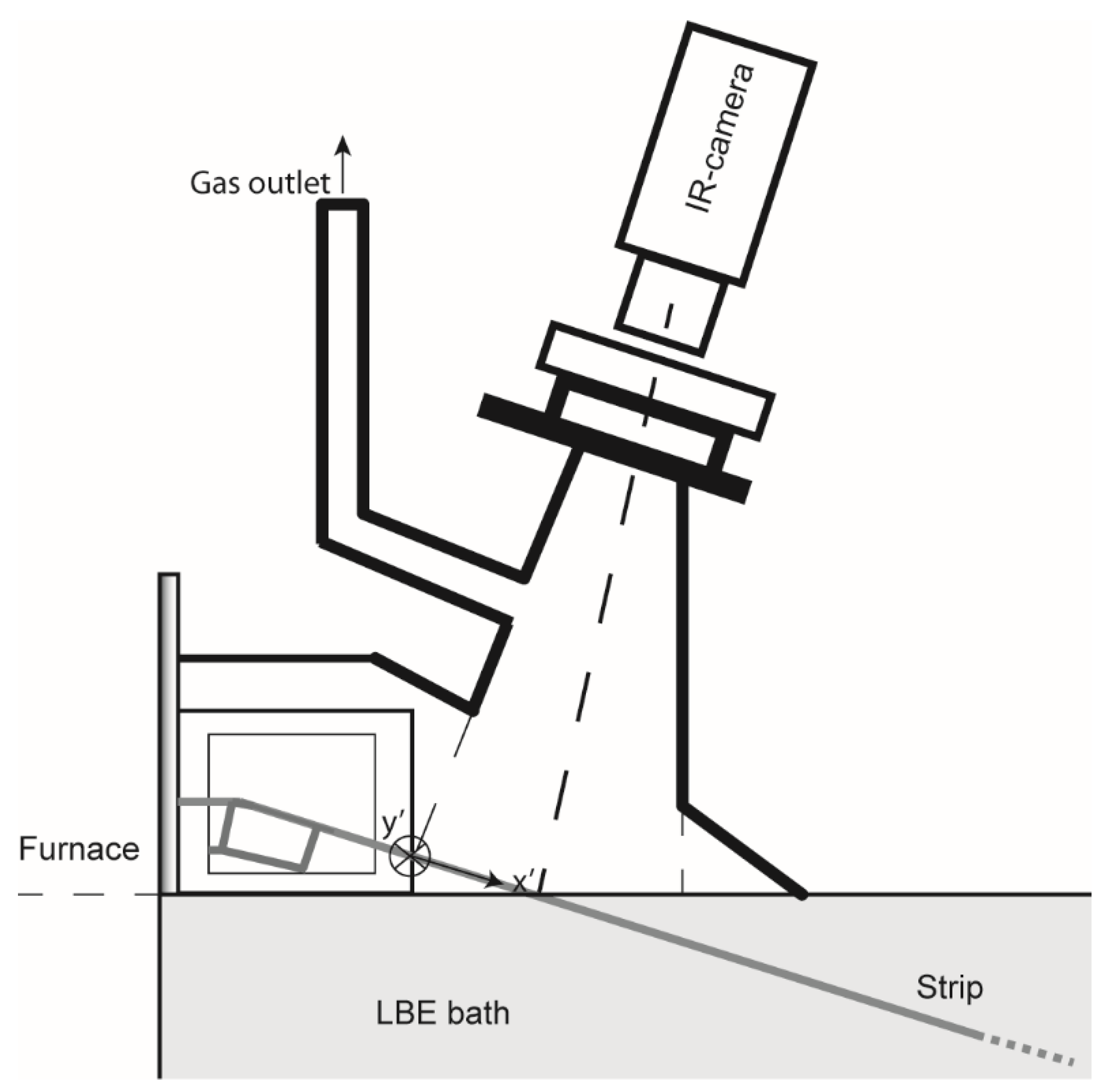
2.2. Temperature Measurements

The effect of a change in the gas inlet location was investigated by measuring the temperature distribution of a chromium stainless steel. For two locations the temperature was measured precisely before the strip entered to the LBE bath during a continuous hardening process. A schematic view of the temporary installation design for the thermal imaging camera is shown in Figure 1. The PYROVIEW 320 thermal imaging camera (DIAS Infrared GmbH, Dresden, Germany) with 320 × 256 pixels and a measuring range of 300 to 1200 °C was mounted on the top of the ceiling of the chamber where the outlet of the furnace gas flow is also located. The dimensions of the stainless steel strip are 0.2 mm thickness and 310 mm width. As can be seen in Figure 1, the strip quenches at x′ direction by the LBE bath. Furthremore, the measured temperature data was achieved during steady state condition of the continuous hardening process. The camera installations and settings were considered in compliance to the previous measurements done by the current research group [16], which included an emissivity value of 0.4. According to the manufacturer [17] the measurement uncertainty is ±2% of the measured value.

3. Mathematical Model

3.1. Mathematical Formulation

The numerical model of this study was conducted in three-dimensional (3D). Moreover, the stainless steel strip, sealed metal bath including the hydrogen gas flow, gliding material, and LBE bath were accounted for in the mathematical model. In addition, the computational model was based on the following statements and assumptions:
(a)
A laminar non-isothermal hydrogen flow was considered in the study (because of Reynolds number, calculated based on the inlet).
(b)
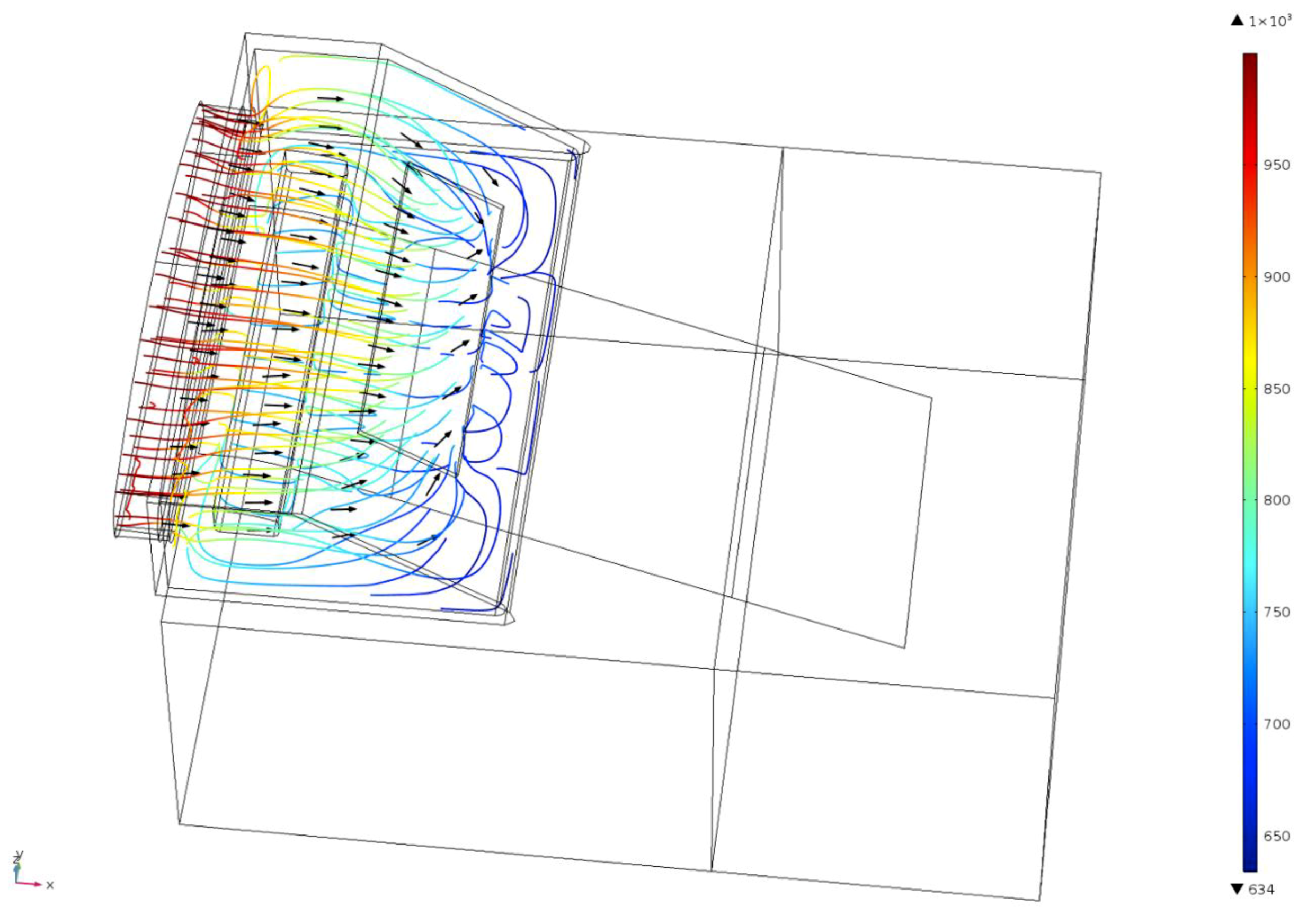
Within the hydrogen filled sealed box domain, the laminar Navier–Stokes equation was solved numerically in combination with the energy balance and continuity equation. Thus, within the sealed box a thermal interaction between the hydrogen flow and the strip takes place.
(c)
The thermal interaction between the strip and the molten metal bath was investigated by only considering heat conduction.
(d)
Steady state was assumed and therefore the transient effects (time dependency) were neglected.
(e)
The gravitational force was neglected.
Based on these assumptions the following governing equations were solved numerically:
  • Continuity equation:
    · ( ρ u ) = 0
    where ρ is the mass density (kg/m3) and u is the velocity vector (m/s).
  • Momentum equation:
    ρ u · u = p + · ( μ ( u + ( u ) T ) 2 3 μ ( · u ) I )
    where T is the transpose matrix, p is the pressure (Pa), μ are the dynamic viscosity of the fluid [Pa·s] and I stands for the identity matrix.
  • Energy balance equation:
    ρ c p u · T = · ( k T )
    where, c p defines the heat capacity at a constant pressure (J/kg·K), k represents the thermal conductivity (W/ (m·K)) and T is the temperature (K).

3.2. Boundary Conditions and the Initial Values

The computational domain solved in this study is shown in Figure 2. In this research, the surface A was considered as an alternative position of the gas inlet. Surface B stands for the outlet of the numerical model. As it can be seen in Figure 2, a 0.2 mm stainless steel strip is located at the top part of the gliding material within two domains, namely the sealed metal box and the LBE bath. Details of the size of LBE bath, stainless steel strip and the gliding material together with the physical properties of the hydrogen, wall of the sealed metal box, LBE, stainless steel strip and the gliding material used for the model are described in details in reference [16]. The dimensions of the sealed metal box are given in Table 1.
Different boundary conditions were set for solving the numerical 3D model, which were chosen to describe the thermal interaction at the various domains. Specifically, the following statements and assumptions define the boundary conditions of the model:
  • A no–slip boundary condition for the inner side of the ceiling of the metal box. u = 0
  • A moving wall for the strip parts located inside the sealed metal box. The value is the same as the velocity of the strip in the process. u u , d = v S t r i p   m / s   ( < 0.17   m / s ) where u , d is u p ,   d o w n .
The effect of the strip velocity was studied numerically and the following strip velocities were used in this investigation: v S t r i p 1 30 m/s, v S t r i p 1 60 m/s, v S t r i p + 1 60   m / s , v S t r i p + 1 30 m/s.
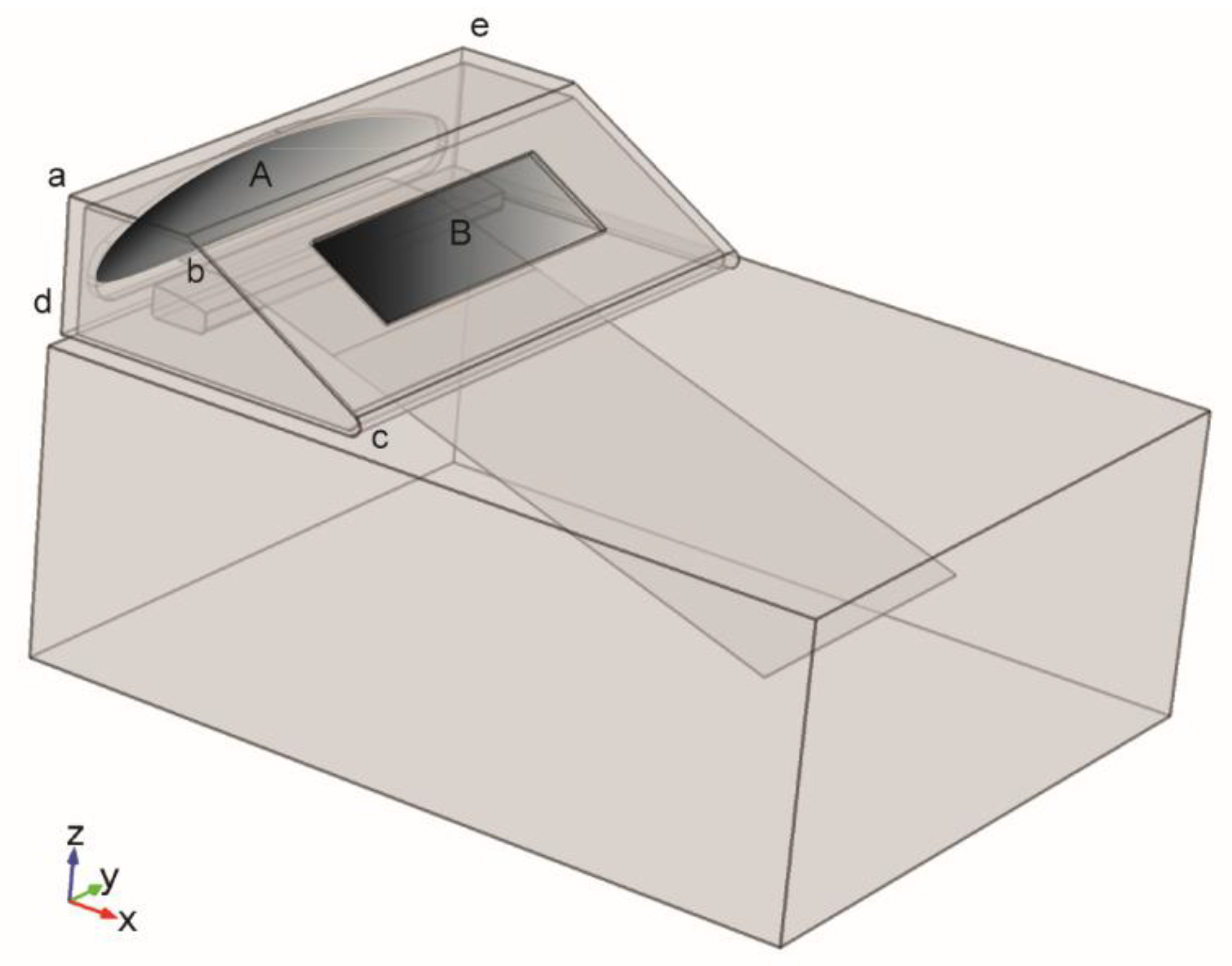
  • A velocity gas inlet for the surface A in Figure 2 = v g a s , Q = 2.66 Nm3/h, v = Q g a s   ( a t   1000   )   A r e a = 0.108 m/s, Moreover, different flow rates for hydrogen gas were investigated numerically in order to determine the impact of this parameter on the predictions. The values 1.66 Nm3/h, 3.66 Nm3/h and 4.66 Nm3/h were assumed in the parametric study.
  • A typical furnace temperature for the Surface A and its connected surface. T A = 1000   °C.
  • A pressure outlet at the Surface B in Figure 2 where a backflow is allowed.
  • A convective heat flux for the outside the ceiling part of the sealed box.
    k T = h . ( T e x t e r n a l T ) , T e x t e r n a l = 20 °C assumed heat transfer coefficient h = 0.5 W·m–2·K–1.
  • A surface to surface radiation for the inner side of the ceiling of the gas box, surface of the strip, and the surface of the LBE bath in the sealed metal box. k T = ε . ( G σ T 4 ) [18].
    ε : surface emissivity, G : incoming radiative heat flux W·m–2, σ : Stefan–Boltzmann W·m–2·K–4.
  • A typical set point temperature for the bath. T b a t h = 300 °C. Details of the choosing the proper bath boundary condition is described in details in reference [16].
  • A convective heat flux for the top surface of the bath, outside area of the sealed metal box.
    T e x t e r n a l = 20 °C, a low value of h due to oxidation, h = 0.1 W·m–2·K–1 is assumed.

3.3. Numerical Conditions

The mathematical model was solved numerically by using the three dimensional (3D) Comsol Multiphysics software [19]. The predictions were made using three different numbers of grid elements, i.e., 79, 570, 341,133, and 561,391. This was carried out in order to improve the calculation time and to obtain mesh independent results. In addition, an unstructured grid was used for this model, which included various element shapes such as tetrahedral, pyramid, triangular, edge, prism, and vertex. A typical calculation took 1.5 h on a custom built Win7 PC from various parts, equipped with a 3.40 GHz Intel Core i7 CPU and a 32 GB RAM.

4. Results and Discussion

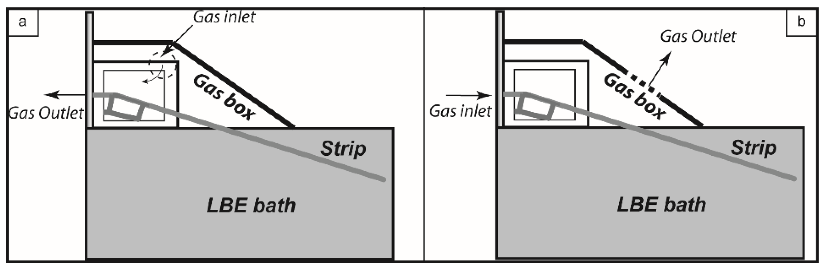
4.1. The Impact of the Alternative Placement of the Gas Inlet

The impact of the change in the gas inlet location was our focus of this study. The results of the predicted model with an alternative gas inlet location together with the model validation are presented in this section. The boundary conditions used for the investigation were described briefly in chapter 3.2. The following parameters were considered for the numerical model and the temperature measurement results represented in the current chapter:
  • Gas inlet position: Surface A in Figure 2.
  • Gas outlet position: Surface B in Figure 2.
  • Strip velocity: v S t r i p (m/s) ( < 0.17   m / s ) .
  • Hydrogen flow rate: Q = 2.66 Nm3/h

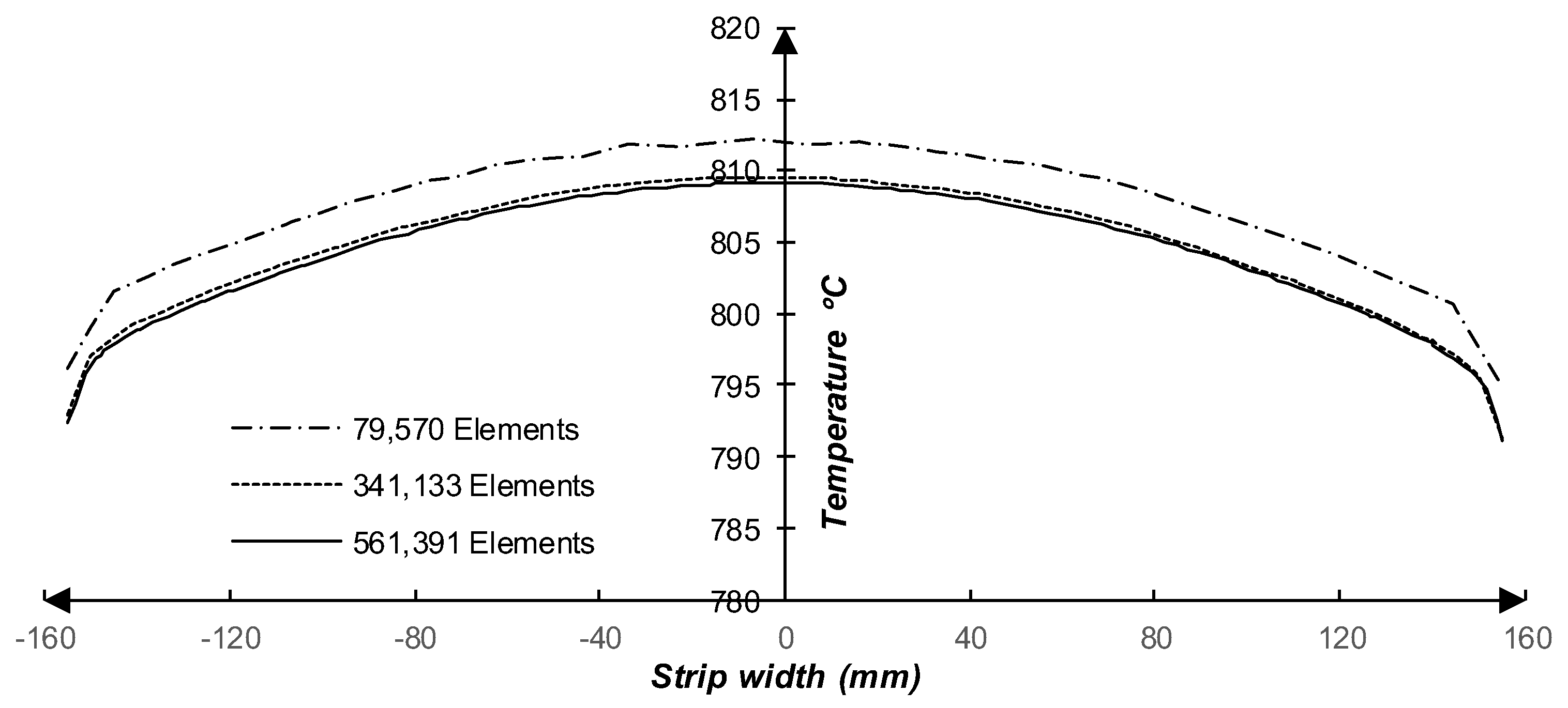
4.1.1. Grid Sensitivity Study

In order to achieve mesh independent results and to improve the convergence time, three different number of grid elements were applied in the model. Moreover, a mesh analysis was conducted by comparing the strip temperatures along a line through the y-direction (strip width) located 70 mm before the entrance to the LBE bath. The result is shown in Figure 3. By comparing the maximum temperature values, it can be seen that there is about a 0.39% deviation between the meshes containing 79,570 and 561,391 elements, while a 0.05% deviation is found between the meshes containing 341,133 and 561,391 elements. Furthermore, the computational time is 3 times smaller for a 341,133 mesh than the time needed for solving a 561,391 mesh. Therefore, an unstructured grid with 341,133 elements was selected as the proper mesh for the remaining part of the study.

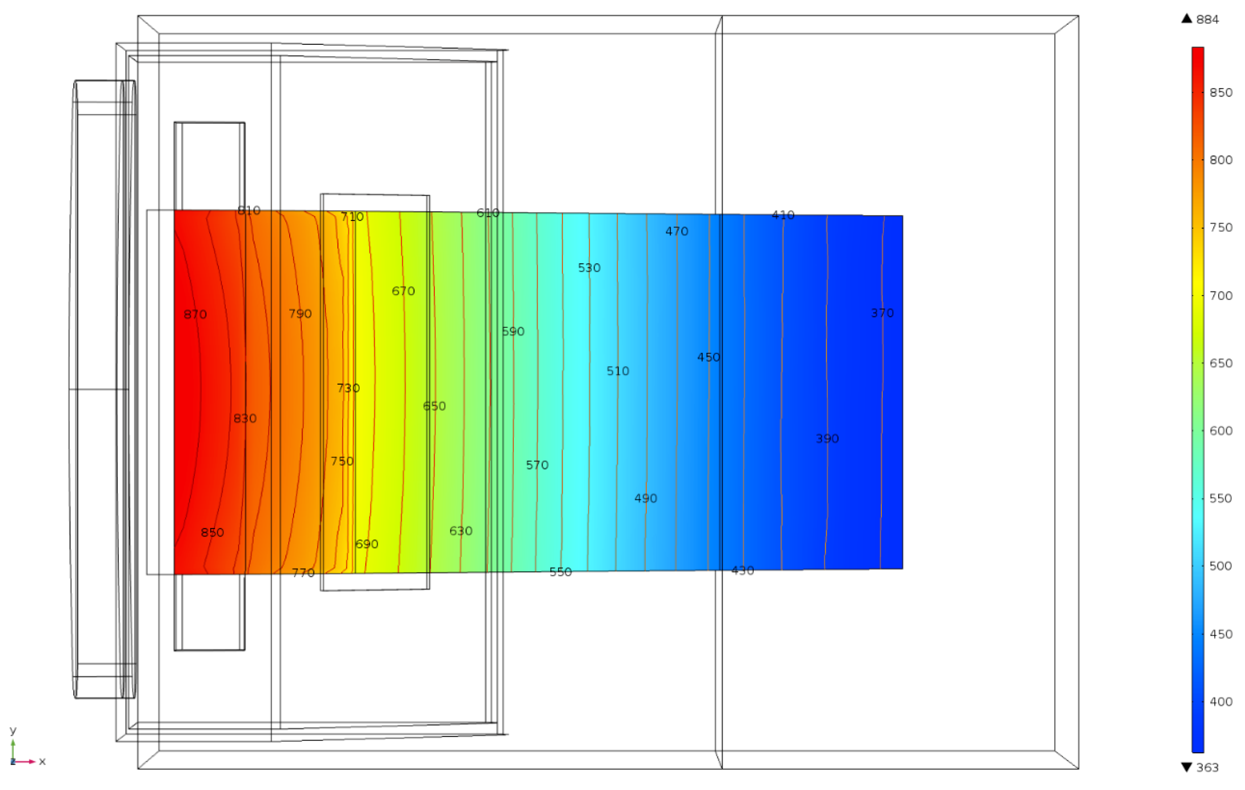
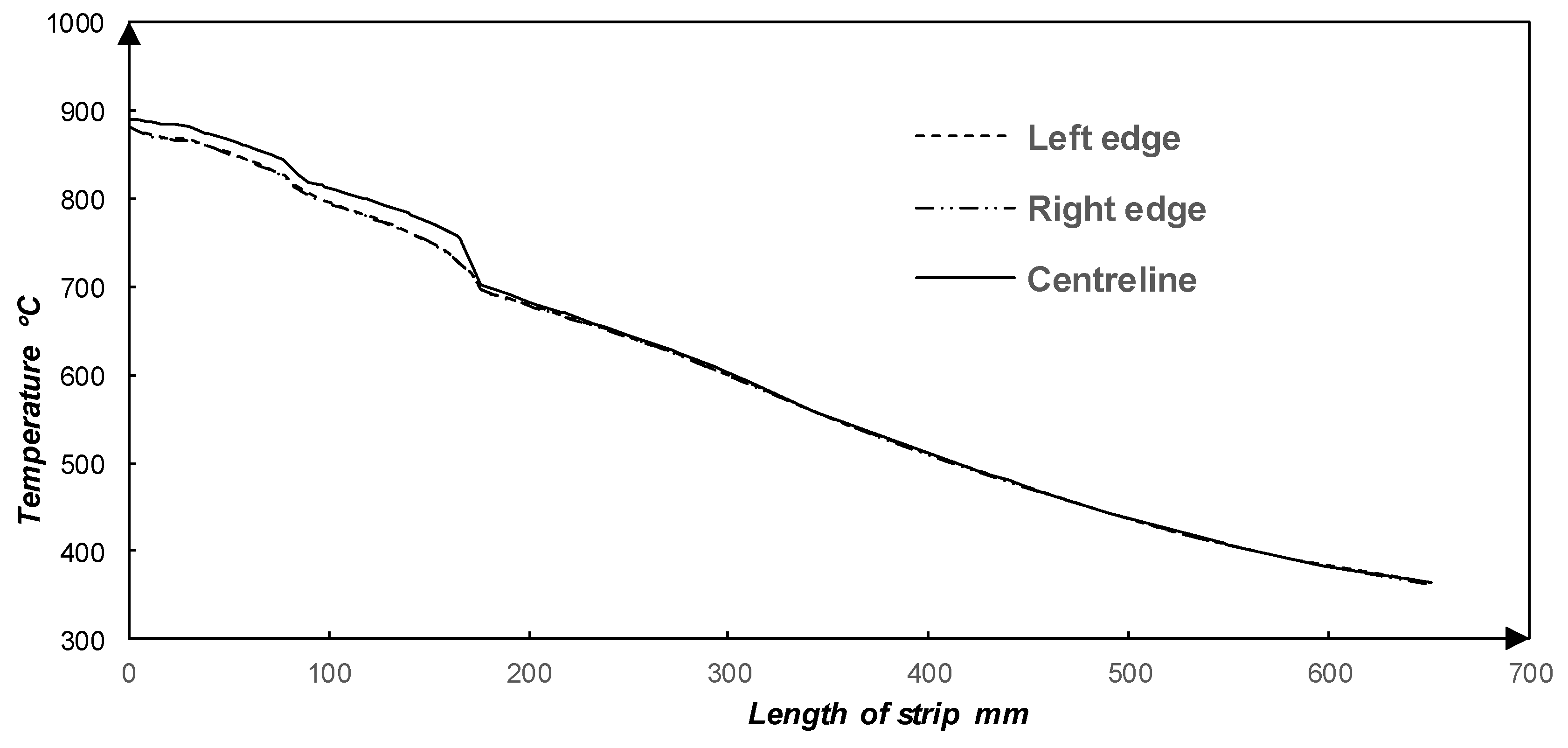
4.1.2. Numerical Model Predictions

The predicted hydrogen flow patterns from the numerical model simulations are illustrated in Figure 4. The color of the lines represents their corresponding temperatures. Overall, symmetric flow trajectories can be seen. Meanwhile, the temperature of the gas decreases dramatically within the sealed metal box. One reason is the thermal interaction of the flow with the surface of the LBE bath. In addition, a convective heat flux from the ceiling of the box to the surroundings causes a decrease in the temperature of the flow.
Figure 5 illustrates the predicted temperature patterns together with the temperature contour plots for a stainless steel strip.
In addition, Figure 6 presents the temperature trajectories of the strip at its edges and the center, along the length of the strip. A symmetrical temperature distribution appears in the strip. Meanwhile, a noticeable transverse temperature differences (y-direction) can be observed in the strip before a further cooling takes place by the LBE. Specifically, the temperature differences can be up to about 42 °C in the length position of 171 mm, where the strip hits the LBE bath at the length position of 175 mm. In addition, a significant decrease of the temperature of strip can be noticed. Particularly, the temperature of the center of the strip decreases from 1000 °C (a typical furnace temperature) to about 755 °C at a distance 10 mm before the strip enters to the molten metal bath. Furthermore, a uniform temperature distribution can be found in the strip parts, which are immersed in the bath.

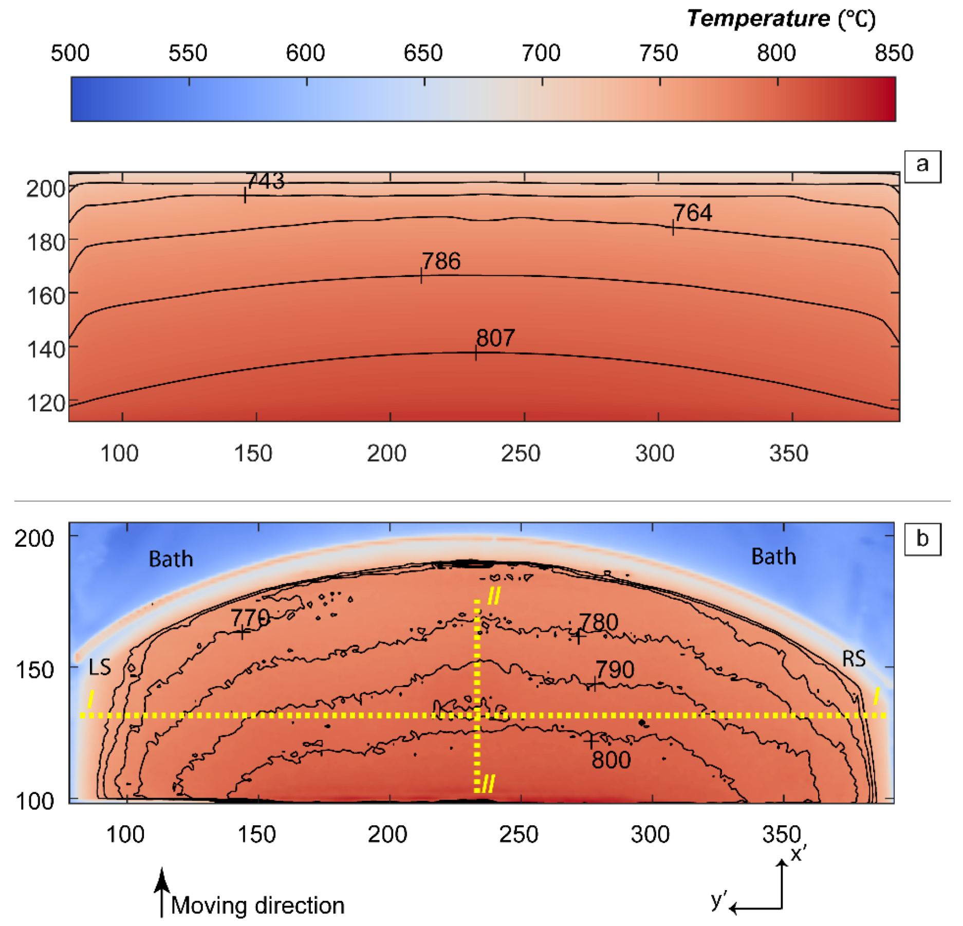
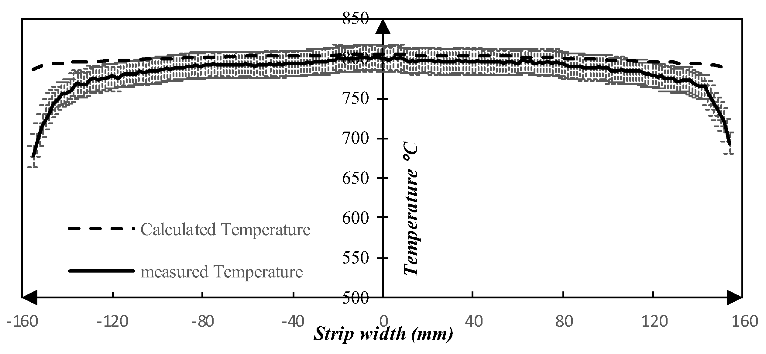
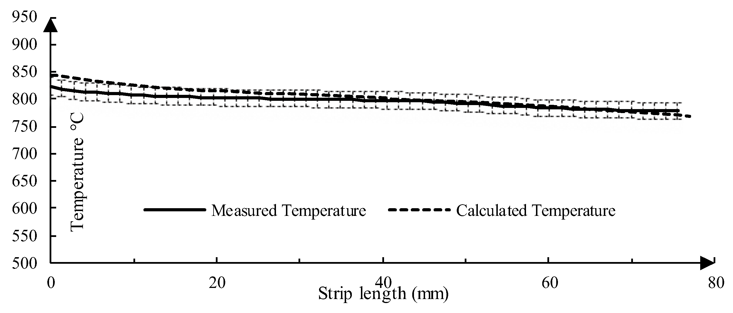
4.1.3. Validation of the Model

In order to validate the model, infrared thermal imaging was employed. A direct comparison of the results of the predicted model and the real process temperature measurements with their temperature contours are represented in Figure 7. The predicted temperature resulted from the numerical model is shown in Figure 7a. These results are limited to the area where the temperature measurements had been performed. Furthermore, Figure 7b shows the result of the measured temperature in the real process. The abbreviations LS and RS stand for the left-hand side and right-hand side of the strip, based on its moving direction respectively. Two lines, shown as I–I and II–II in Figure 7b were used for the comparison between the calculated and measured temperature values across the transverse direction (the width of strip) and longitudinal direction (along the length of strip), respectively. The curved shape of the strip at the entry to the bath implies that a buckling of the strip had occurred. The results show that the temperature of the strip decreases dramatically within the sealed metal box. As it can be seen in Figure 7b, the temperature of the strip decreases to about 770 °C from the furnace temperature, i.e., 1000 °C, within the metal box and beyond the cooling in the LBE bath. In addition, a symmetrical temperature distribution can also be observed. The warmest area of the strip is found to be located at the center of the strip.
Figure 8 expresses the temperature distribution along the I–I line resulting from both the predicted model and the measured values. This line is located at a position of about 63 mm from the bath interface. Furthermore, the measurement uncertainty, ±2% of measured value, is shown as an error bar. It can be seen that the maximum temperatures are very similar, namely 804 °C and 802 °C for the predicted and measured values respectively. The maximum deviation of the calculated values to the measured temperature is 16.0% located at the edges of the strip.
Despite of the same temperature pattern, different values for the temperature were observed specifically at the edges by comparing the calculated results with measured data. This can be explained by the available uncertainty and errors in the IR-camera temperature measurements. Dias [17] introduced ±2% of the measured value as the uncertainty of the measurement. This level of uncertainty should be considered as a minimum value, as it was determined for an operation of the camera under specified laboratory conditions. More specifically, Dias [17] measurements were done at an ambient temperature of 25 °C and for a black body radiator. Thus, for practical measurements this error maybe significantly higher. This issue and other errors in connection with infrared temperature measurements were discussed by Minkina and Dudzik [20]. More details regarding the errors of the measurements are available and briefly discussed in the previous work done by the same research group [16]. It has to be mentioned that finding the same line for the comparison between the calculated results and the measured value is extremely difficult. Also, a higher cooling at the very edges may resulted from a possible localized turbulence.
Due to the limitations of performing temperature measurements by using an IR camera specifically at the edges, the comparison of the temperature between the measured and model values were conducted by excluding the data from a position at around 20 mm from each edge in Figure 8. The minimum values were 796 °C and 767 °C for the calculated temperatures and measured values, respectively. Therefore, the maximum deviation between the calculated temperatures and the measured values decreases from 16.0% to 3.7%. Therefore, the agreement between the predictions and measurements is deemed to be acceptable.
Figure 9 shows the temperature of the strip along the longitudinal direction. Line II–II with the length of 77, ended at 21 mm before the bath entry. At this specific line, the temperature of the strip decreases from 845 °C to 769 °C, based on the numerical calculations. Meanwhile, due to the empirical measurements, the temperature declines from 823 °C to 777 °C. Therefore, a proper agreement is visible for the temperature values resulting from the numerical model and the measured data. In addition, the same tendency can clearly be seen from the results from both methods.

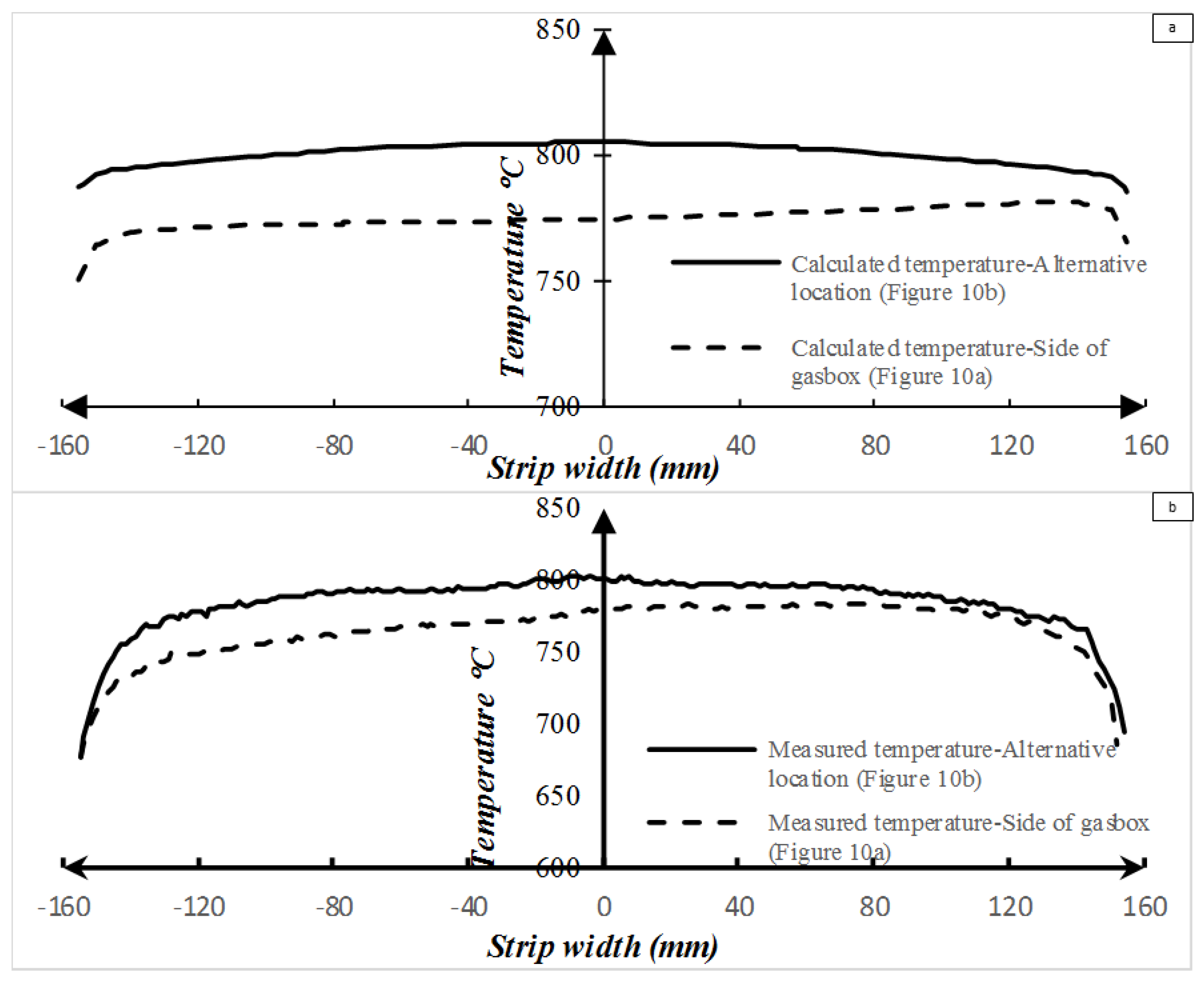
4.1.4. Comparison between Two Gas Inlet Positions

The schematic view of two gas inlet and outlet locations in the process are shown in Figure 10. Figure 10a represents a schematic view of the location of the gas inlet, where it is located in the side of sealed metal box or namely in the gas box. This case was investigated previously by the current research group [16] both numerically and empirically. Furthermore, the schematic view of using the alternative gas inlet position i.e., Surface A in Figure 2 in the process is shown in Figure 10b. The current case was studied in this research and the results were shown in chapter 4.1.2 and 4.1.3. Hence, the results between two cases are compared and shown in Figure 11. This was done by measuring the temperatures of the strip along the vertical line, the I–I line in Figure 7b, at a position 63 mm before the entrance to the LBE bath.
It can be seen in Figure 11 that a more symmetrical and uniform temperature distribution can be seen in the strip by considering surface A in Figure 2 as the inlet (Figure 10b case) instead of at the side of the sealed metal box (Figure 10a case). The details regarding the temperature values shown in Figure 11 are given in Table 2, where the data at 20 mm from each edge was ignored due to the limitation of IR temperature measurements. By using an alternatively located hydrogen gas inlet (Figure 10b case), the maximum temperature of the strip at the I-I line was increased by 3.1% and 2.3% based on the predicted results and the measured values, respectively. Therefore, by considering a specific furnace temperature, i.e., 1000 °C, as the initial temperature of the strip, a higher amount of lost heat can be seen by using a metal box gas inlet method (Figure 10a case). Furthermore, by placing a hydrogen inlet of in the alternative location (Figure 10b case), a smaller temperature difference across the transverse direction (width of strip) together with a symmetrical temperature pattern can be achieved. Specifically, the temperature difference was decreased by 9% and 14% due to the calculated temperature and measured values respectively. Therefore, a new placement of the hydrogen gas inlet is more desirable.

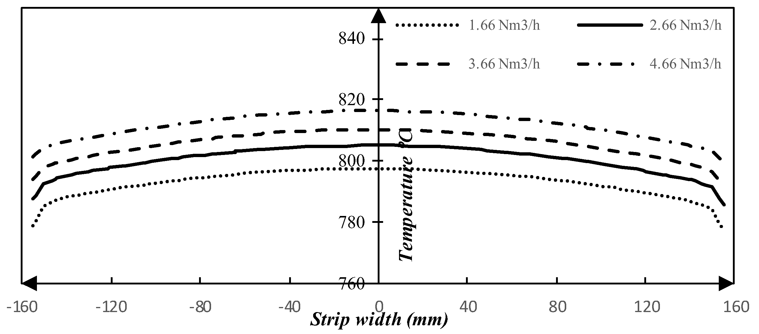
4.2. The Impact of the Different Hydrogen Flow Rate

The effect of the different flow rates of hydrogen gas on the strip temperature was investigated numerically. To determine the effect, the temperature across the width of strip at a position 63 mm from the bath interface are shown in Figure 12 and explained in Table 3.
It can be seen that the temperature of the strip increases by 11 °C or 1.4% by increasing the hydrogen flow rate by 2 Nm3/h. In addition, a lower temperature differences across the width of strip is predicted by the mathematical model. More specifically, the difference is 4 °C or 20% lower. This is due to that a higher amount of warm hydrogen gas is created in the metal box, which contributes to a heating of the strip.

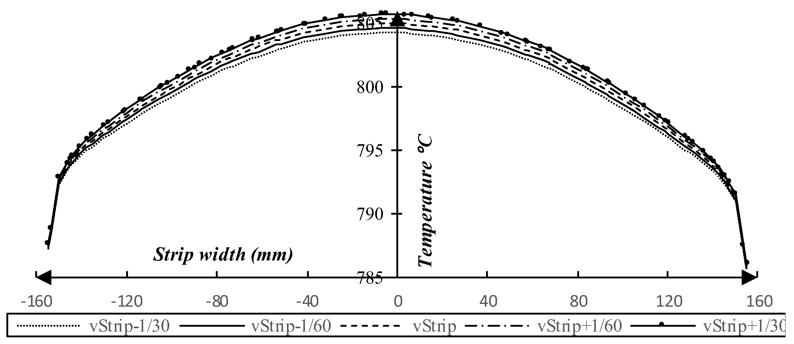
4.3. The Impact of the Different Strip Velocity

Different values for the strip velocity were assumed to study the effect of this variable on the temperature distribution. The temperatures across the width of the strip at a position 63 mm from the LBE bath interface are shown by Figure 13 and explained in Table 4. It can be seen that the effect of the strip velocity on the strip temperature is very little. Furthermore, it has been observed by the predicted model that by increasing 0.03 m/s or 2 m/min to the process velocity ( v S t r i p < 0.17   m / s ) , the maximum temperature increases by 0.8 °C or 0.1%. Meanwhile, the temperature differences across the width of strip increases very slightly by up to 0.3 °C or 0.03%. This tiny increase in the maximum temperature is due to the existence of shorter cooling time in the sealed metal box, because of a higher velocity of the strip.

5. Conclusions

A model of the heat treatment process was made to study the effect of an alternative position of the gas inlet on the temperature distribution of the steel strip. This was done based on mathematical modelling. In addition, thermal imaging was used in order to compare the predicted results to the real process measurements. Moreover, the influence of the variation of the hydrogen flow rate on the strip temperature as well as the strip velocity were studied based on a numerical parameter study. Furthermore, the results of this study were compared to the results from a previous study. The main conclusions are the following:
  • By using an alternate gas inlet and position, where the main gas flow is in the same direction as the strip as opposed to a crossflow scenario, a significant higher degree of symmetry with respect to temperature is achieved along the transverse direction (width of strip). Specifically, the difference of the temperature in the transverse direction (width of strip) decreased by 9% and 14% based on the calculated temperature and measured values, respectively.
  • Increasing the hydrogen flow rate, a reduction of the temperature difference across the transversal direction, close to the bath interface is observed. Specifically, by increasing the flow rate by 2 Nm3/h, the transverse temperature difference decreased by approximately 20%. Thus, a higher gas flow rate promotes a smaller temperature difference along the width of the strip.
  • A parametric study of the strip velocity showed that by increasing the velocity of the strip in the process by 2 m/min, the maximum temperature at close to the bath interface increases marginally. Thus, the effect of the strip velocity on the strip temperature is quite small.

Author Contributions

Conceptualization: N.Å.I.A. and A.T.; methodology: P.P., N.Å.I.A. and A.T.; validation: P.P., N.Å.I.A. and A.T.; formal analysis: P.P., N.Å.I.A. and A.T.; investigation: P.P.; resources: A.T., P.G.J.; data curation: P.P.; writing–original draft preparation: P.P.; writing—review and editing: P.P., N.Å.I.A., A.T. and P.G.J.; visualization: P.P. and N.Å.I.A.; supervision: N.Å.I.A. and A.T.; project administration: A.T.; funding acquisition: A.T.

Acknowledgments

The authors would like to thank Chris Millward and Stellan Ericsson of voestalpine Precision Strip AB, for fruitful discussions and a great support to carry out the temperature measurements as well as Nihat Palanci of Sensotest, Sweden for providing the possibility to use the Infrared camera for the industrial measurements. This study was carried out with a financial support from the Regional Development Council of Dalarna, The Regional Development Council of Gävleborg, The County Administrative Board of Gävleborg, the Swedish Steel Producers’ Association, Dalarna University, Sandviken Municipality, and voestalpine Precision Strip AB.

Conflicts of Interest

The authors declare no conflict of interest.

References

  1. Webster, H.; Laird, W.J. Martempering of Steel, Heat Treating. In ASM Handbook; ASM International: Materials Park, OH, USA, 1991; Volume 4, pp. 137–151. [Google Scholar]
  2. Ebner, J. Bright Heat Treating of Carbon Steel Strip Using a Lead Quench. Mach. Steel Austria 1983, 4, 83–90. [Google Scholar]
  3. Lochner, H. Hardening of strip in a molten-metal bath or hydrogen jet cooler. Steel Times 1994, 222, 350. [Google Scholar]
  4. Lochner, H. Steel strip hardening and tempering lines for medium and high carbon steels and alloyed grades part I: Production lines with liquid metal quenching. In Proceedings of the IFHTSE—International Federation for Heat Treatment and Surface Engineering, Vienna, Austria, 25–29 September 2006; p. 43. [Google Scholar]
  5. Thelning, K.-E. 7-Dimensional changes during hardening and tempering. In Steel and its Heat Treatment, 2nd ed.; Butterworth-Heinemann: Oxford, UK, 1984; p. 581. [Google Scholar]
  6. Yoshida, H. Analysis of Flatness of Hot Rolled Steel Strip after Cooling. Trans. Iron Steel Inst. Jpn. 1984, 24, 212–220. [Google Scholar] [CrossRef]
  7. Wang, S.-C.; Chiu, F.-J.; Ho, T.-Y. Characteristics and prevention of thermomechanical controlled process plate deflection resulting from uneven cooling. Mater. Sci. and Technol. 1996, 12, 64–71. [Google Scholar] [CrossRef]
  8. Wang, X.; Yang, Q.; He, A. Calculation of thermal stress affecting strip flatness change during run-out table cooling in hot steel strip rolling. J. Mater. Proc. Technol. 2008, 207, 130–146. [Google Scholar] [CrossRef]
  9. Wang, X.; Li, F.; Yang, Q.; He, A. FEM analysis for residual stress prediction in hot rolled steel strip during the run-out table cooling. App. Math. Model. 2013, 37, 586. [Google Scholar] [CrossRef]
  10. Guarino, S.; Barletta, M.; Afilal, A. High Power Diode Laser (HPDL) surface hardening of low carbon steel: Fatigue life improvement analysis. J. Manufac. Proc. 2017, 28, 266–271. [Google Scholar] [CrossRef]
  11. Idan, A.F.І.; Akimov, O.; Golovko, L.; Goncharuk, O.; Kostyk, K. The study of the influence of laser hardening conditions on the change in properties of steels. East Eur. J. Adv. Technol. 2016, 2, 5. [Google Scholar] [CrossRef]
  12. Rappaz, M. Modelling of microstructure formation in solidification processes. Int. Mater. Rev. 1989, 34, 93–124. [Google Scholar] [CrossRef]
  13. Choudhary, S.K.; Mazumdar, D.; Ghosh, A. Mathematical Modelling of Heat Transfer Phenomena in Continuous Casting of Steel. ISIJ International 1993, 33, 764–774. [Google Scholar] [CrossRef]
  14. Koric, S.; Hibbeler, L.C.; Liu, R.; Thomas, B.G. Multiphysics Model of Metal Solidification on the Continuum Level. Numer. Heat Transf. Part B Fundam. 2010, 58, 371–392. [Google Scholar] [CrossRef]
  15. Eriksson, S. (R&D Process Technology, Voestalpine Precision Strip AB, Munkfors, Sweden). Personal communication, 2012. [Google Scholar]
  16. Pirouznia, P.; Andersson, N.Å.I.; Tilliander, A.; Jönsson, P.G. An investigation of the Temperature Distribution of a Thin Steel Strip during the Quenching Step of a Hardening Process. Metals 2019, 9, 675. [Google Scholar] [CrossRef]
  17. DIAS Infrared Systems. Available online: http://www.webcitation.org/785ncpRm6 (accessed on 3 May 2019).
  18. Multiphysics, C. Heat Transfer Module User’s Guide; Version 5.1; COMSOL AB: Stockholm, Sweden, 2015. [Google Scholar]
  19. COMSOL. COMSOL Multiphysics v.5.1. Available online: https://www.comsol.se/release/5.1 (accessed on 3 May 2019).
  20. Minkina, W.; Dudzik, S. Errors of Measurements in Infrared Thermography. In Infrared Thermography; John Wiley & Sons, Ltd.: Hoboken, NJ, USA, 2009; p. 61. [Google Scholar]
Figure 1. Schematic view of the setup for the temperature measurements at the hardening process. LBE: lead-bismuth eutectic.
Metals 09 00928 g001
Figure 2. View of domain shapes.
Metals 09 00928 g002
Figure 3. Mesh analysis of the numerical model based on a comparison of the strip temperatures along a line through the y-direction (strip width) located 70 mm before the entrance to the LBE bath.
Metals 09 00928 g003
Figure 4. Numerical results of the hydrogen gas flow with its temperature (°C). Gas inlet position: surface A in Figure 2, Q = 2.66   Nm 3 / h , Strip velocity = v S t r i p ( < 0.17   m / s ) .
Metals 09 00928 g004
Figure 5. A contour plot of the temperature of the strip (°C). Gas inlet position: surface A in Figure 2, Q = 2.66   Nm 3 / h , Strip velocity = v S t r i p ( < 0.17   m / s ) .
Metals 09 00928 g005
Figure 6. Temperature distribution along the edges and the centre of the strip (°C). Gas inlet position: surface A in Figure 2, Q = 2.66   Nm 3 / h , Strip velocity = v S t r i p ( <   0.17   m / s ) .
Metals 09 00928 g006
Figure 7. Temperature results (a) predicted result from the model and (b) measured temperature by the IR-camera in °C, ε = 0.4. Gas inlet position: surface A in Figure 2, Q = 2.66   Nm 3 / h , strip velocity = v S t r i p ( < 0.17   m / s ) .
Metals 09 00928 g007
Figure 8. Comparison between the model and measured values in the transverse direction, line I–I in Figure 7b. Gas inlet position: surface A in Figure 2, Q = 2.66   Nm 3 / h , Strip velocity = v S t r i p ( < 0.17   m / s ) .
Metals 09 00928 g008
Figure 9. Comparison between the model and measured values in the longitudinal direction, line II–II in Figure 7b. Gas inlet position: surface A in Figure 2, Q = 2.66   Nm 3 / h , Strip velocity = v S t r i p ( < 0.17   m / s ) .
Metals 09 00928 g009
Figure 10. Schematic view of different positions of the gas inlet and outlet. (a) Gas inlet from side of the gas box [16] (b) An alternative location of the gas inlet focused in the current study.
Metals 09 00928 g010
Figure 11. Comparison between the different position of the hydrogen gas inlet, (a) calculated temperatures, and (b) measured temperatures by using the IR-camera, ε = 0.4. Strip velocity = v S t r i p ( < 0.17   m / s ) .
Metals 09 00928 g011
Figure 12. The effect of different hydrogen flow rates on the temperature of strip. Gas inlet and outlet position: Figure 10b, Strip velocity = v S t r i p ( < 0.17   m / s ) .
Metals 09 00928 g012
Figure 13. The effect of different strip velocities on the strip temperature. Gas inlet and outlet position: Figure 10b.
Metals 09 00928 g013
Table 1. Geometry specifications of the sealed metal box (mm). The distances are defined in Figure 2.
a b ¯ . b c ¯ c d ¯ a d ¯ a e ¯ A (mm2)B (mm2) 1 R c ¯
129.8222.6317.6130.0585.031,780334 × 10210
1 R: radius.
Table 2. Temperature comparison between different locations of hydrogen gas inlet by neglecting 20 mm from each sides.
Location of Gas Inlet T m a x ( ° C ) T m i n ( ° C ) Δ T   ( ° C )
Calculated Temperature
Figure 11a
Alternative location (Figure 10b)80579510
Side of gas box [16]
(Figure 10a)
78177011
Measured Temperature
Figure 11b
Alternative location (Figure 10b)80276735
Side of gas box [16]
(Figure 10a)
78474341
Table 3. Temperature values resulted from the different volumetric hydrogen flow rates at the specific position.
Volumetric Flow Rate (Nm3/h) T m a x
°C
T m i n   ( ° C ) Δ T   ( ° C )
1.6679877721
2.6680578520
3.6681079218
4.6681680016
Table 4. Temperature values resulting from the different strip velocities at the specific position.
The Velocity of the Strip (m/s) T m a x   ( ° C ) T m i n   ( ° C ) Δ T   ( ° C )
v S t r i p 1 30 804.3785.618.7
v S t r i p 1 60 804.7785.718.9
v S t r i p 805.0785.819.2
v S t r i p + 1 60 805.4785.919.4
v S t r i p + 1 30 805.8786.119.7

