Quantitative Assessment of the Time to End Bainitic Transformation

Abstract

Low temperature bainite consists of an intimate mixture of bainitic ferrite and retained austenite, usually obtained by isothermal treatments at temperatures close to the martensite start temperature and below the bainite start temperature. There is widespread belief regarding the extremely long heat treatments necessary to achieve such a microstructure, but still there are no unified and objective criteria to determine the end of the bainitic transformation that allow for meaningful results and its comparison. A very common way to track such a transformation is by means of a high-resolution dilatometer. The relative change in length associated with the bainitic transformation has a very characteristic sigmoidal shape, with low transformation rates at the beginning and at end of the transformation but rapid in between. The determination of the end of transformation is normally subjected to the ability and experience of the “operator” and is therefore subjective. What is more, in the case of very long heat treatments, like those needed for low temperature bainite (from hours to days), differences in the criteria used to determine the end of transformation might lead to differences that might not be assumable from an industrial point of view. This work reviews some of the most common procedures and attempts to establish a general criterion to determine the end of bainitic transformation, based on the differential change in length (transformation rate) derived from a single experiment. The proposed method has been validated by means of the complementary use of hardness measurements, X-ray diffraction and in situ high energy X-ray diffraction.

1. Introduction

Bainite implies a displacive transformation involving a sudden, ordered movement of Fe atoms, also accompanied by a crystal correspondence between the parent austenite and the ferrite lattices, and a macroscopic shape strain of the transformed structure [1]. The process is also known to be diffusionless, and therefore, any excess in C present in a bainitic ferrite plate is partially and immediately released to the parent austenite once the plate stops growing [2]. In addition, the precipitation of cementite precipitates from the austenite, inherent to the bainitic transformation, can be retarded or even halted by the use of proper quantities of silicon, i.e., above 1.5 wt.% [3,4]. Thus, finally the microstructure will consist of partially carbon-supersaturated plates of bainitic ferrite, α_b, and C enriched austenite (γ⁺), the latter as thin films between ferrite plates and submicron blocks between sheaves of bainite [5,6]. This microstructure has a high hardness and strength, owing to the combined influence of several types of obstacles to dislocation motion, such as interfaces and dislocations, and also to solid solution strengthening and to the interaction between carbon and defects [3,7,8,9,10,11,12,13,14,15,16,17].

A common way to obtain such a microstructure is by intermediate or low temperature isothermal treatments, above the martensite start temperature (Ms), after full austenitization. In the last decade or so, such treatments have been successfully applied to Si bearing medium–high C steels (0.5–1 wt.%C) in order to obtain the so-called nanostructured bainite [18]. The counterpart in such chemical compositions is the fact that transformation at low temperatures can last from few hours to days [19,20]. Thus, when envisioning the transfer of this novel metallurgical concept to industrial practices, it is important to know and adjust the time of the heat treatments to those strictly necessary—first, because in that type of time-scales, it can imply an important shorten of the whole process, and second, because overextended treatments can lead to further changes in the microstructure, i.e., autotempering and decomposition of the bainitic microstructure [21,22,23].

Through the literature, it is possible to find different methods used to determine the end of the bainite transformation (EBT) [7,24,25], the moment from which there are no more microstructural changes. However, as becomes clear through the text, the process of stablishing an EBT is not free from difficulties and uncertainties and therefore is not trivial.

In this work, the most common approaches are reviewed, for example, determination of the EBT by interrupted isothermal tests, or graphical and simulation methods based on the dilatometric curves obtained during the isothermal treatments. Finally, a method is proposed whose solidity lies in the lack of operator decisions (subjectivity) and in the fact that it does not require “ideal” dilatometric curves.

The scientific community can also gain from the establishment of a standardized method of these characteristics, when discussing and comparing the benefits that certain types of actions, such as chemical composition or prior austenite grain size modifications, the effect of plastic deformation, etc., have in the transformation kinetics of bainite. The described procedure can also be used to get to know, using the dilatometry curve of a single isothermal test, if the bainitic transformation is finished or more time is required.

2. Materials and Methods

For the purpose of this work, and to take into account any possible differences related to the carbon content and, in turn, transformation temperatures and kinetics of bainitic transformation, two steels with different carbon contents were selected. Their chemical compositions are given in

Table 1. Chemical composition of the steels in wt.%, with Fe to balance, and experimental martensite start temperature, Ms in °C.

Alloy	C	Si	Mn	Cr	Mo	Ni	Cu	Ms
Steel 1	0.43	3.05	0.71	0.98	0.21	0.09	0.14	280
Steel 2	0.99	2.47	0.74	0.98	0.02	0.12	0.19	173
Steel 3	0.31	1.52	2.44					320

. Steel 1 corresponds to a commercial steel (SCM40), while Steel 2 was developed in the frame of an R & D project [26]. Although their carbon contents are rather different, both of them have a similar base composition, with differences in the Si content, but in any case sufficient to prevent cementite formation [3,4].

All heat treatments were performed in a Bahr DIL 805D high-resolution dilatometer using cylindrical samples 4 mm in diameter and 10 mm in length. During dilatometry measurements, the specimen is held between two quartz rods, one fixed and the other connected to a LVDT (linear variable displacement transducer). Thus, during the whole heat treatment, it was possible to measure the relative change in length (RCL) of the sample. Figure 1a shows the sketch of the isothermal heat treatments performed, where T_γ, T_Iso and t_γ, t_Iso are the austenitization and isothermal temperatures and times, respectively. Heating was applied by an induction coil and the temperature controlled by a type K thermocouple spot welded in the center of the specimen. All experiments were carried out in vacuum (10⁻⁴ mbar). All the heat treatment parameters were carefully selected and adapted to the chemical composition of the steels in order to obtain a bainitic structure; the details have been profusely discussed in [20,26,27]. Suffice it to say that in order to study the temporal advance of the bainitic transformation, different times t_Iso were selected, the longest one being enough for the transformation to reach its completion.

The typical sigmoidal curve obtained by dilatometry during isothermal bainitic transformation can be divided into different regions, see Figure 1b [28]:

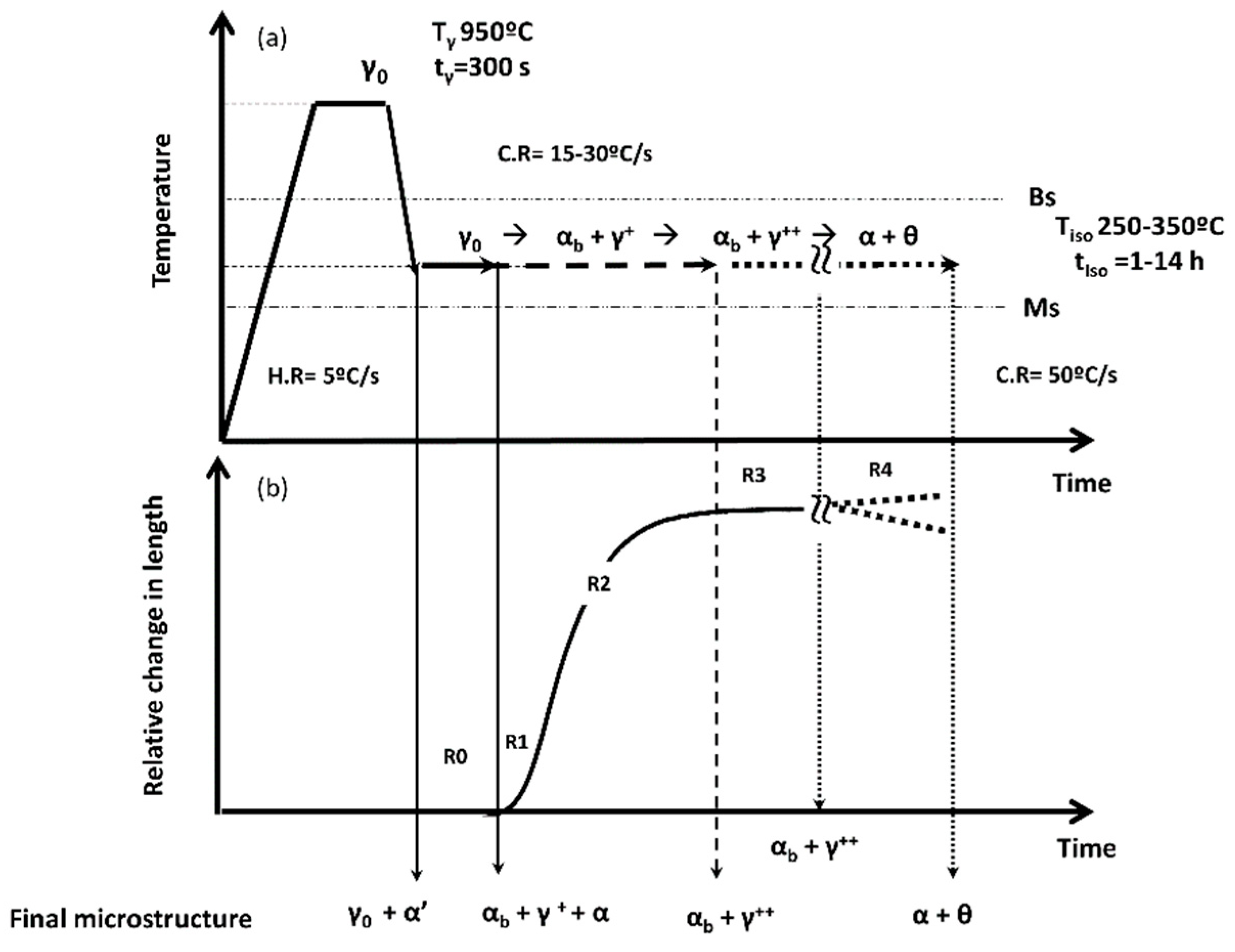
• A first stage, R0, called the incubation period, during which the transformation has not yet started, or it is not yet detectable, and the microstructure remains fully austenitic;
• The transformation period, where nucleation and growth occur, and the microstructure tends to evolve from γ to α_b + γ⁺ (R1 & R2). Differences between R1 and R2 become clear later in the text;
• The last stage in which the signal reaches a steady-state, and transformation does not proceed any further, R3. This region is not always easily identifiable, because in some cases, the RCL signal does not achieve a clear steady-state, but it remains increasing or decreasing with a low but constant slope;
• If treatments are performed for much longer times than necessary, R4, further changes in the microstructure can take place, e.g., autotempering and decomposition of the bainitic microstructure [21,22,23], and discontinuous lines in Figure 1b intend to highlight the fact that the occurrence of those can lead to different outcomes in the dilatometric curve. For example, decomposition of residual austenite into a mixture of ferrite and cementite can lead to a net contraction or expansion depending on the amount of C in solid solution [29], whereas carbon partitioning i.e., further C enrichment of austenite, due to autotempering of bainitic ferrite, will introduce a contraction, and the precipitation of carbides from austenite and bainitic ferrite will induce an expansion and a contraction, respectively.

Thus, somewhere in the third stage (R3), there should be a point where the transformation clearly ends, or at least, from that point on, an increase in the α_b fraction is not detectable by different microstructural characterization techniques.

The evolution of the bainitic microstructure was here evaluated by means of X-ray diffraction and hardness measurements. To this end, samples were prepared following standard metallographic procedures finishing with 1 μm diamond paste. To remove the surface deformed layer due to the metallographic preparation, where austenite may have transformed to martensite under mechanical loading, several etching and polishing cycles were applied before finally polishing with colloidal silica suspension.

X-ray diffraction measurements were carried out with a Bruker AXS D8 diffractometer equipped with a Co X-ray tube, Goebel mirror optics, and a LynxEye linear position sensitive detector for ultra-fast XRD measurements. A current of 30 mA and a voltage of 40 kV were employed as tube settings. XRD data were collected over a 2θ range of 35–135° with a step size of 0.01°.

In this study, version 4.2 of Rietveld analysis program TOPAS (Bruker AXS) was used for phase quantification, as well as for the determination of the lattice parameters. The structural model used in the refinement was a combination of ferrite and austenite. To eliminate the instrumental contribution to peak broadening, instrument functions were empirically parameterized from the profile shape analysis of a corundum sample measured under the same conditions. Further details concerned with the XRD data analysis leading to the determination of the different phase fractions, their corresponding lattice parameters, and the chemical compositions derived are reported elsewhere [6,30,31,32,33,34,35].

Microstructural observation was also performed after etching with Nital 2% using a JEOL J8M-6500 FEG-SEM (JEOL Ltd., Tokyo, Japan) operating at 10 kV.

Vickers hardness measurements, HV, were performed according to the ASTM E92-17 standard using a 10 kg load, the results corresponding to an average of at least three measurements.

For Steel 3, Table 1, an in situ high energy X-ray diffraction (HEXRD) facility, DESY PETRA P07 beamline (Hamburg, Germany), fitted with a dilatometer, which permits following at the same time the metallurgical evolutions in the studied steel and the dilatometer signal with a very good time resolution, was used to validate the proposed method. The in situ experiments were carried out in transmission at high energy (100 keV–400 × 400 µm) using a 2D Perkin-Elmer detector about 1 m behind the sample. The acquisition rate was set to 10 Hz at the beginning of the isothermal step and at 0.3 Hz at maximum. The sample was heated in a commercial Bahr DIL 805D available on the line, and the experimental set up was identical to that already described. The 2D diffraction patterns (Debye-Scherrer rings) were then circularly integrated, and each corresponding 1D diffractogram underwent a Rietveld analysis to determine the respective fraction of phases in the sample (bainite and austenite) all along the isothermal treatment. Steel 3 is a model alloy developed in the frame of an ongoing research, and further details of its development and characteristics can be found elsewhere [36,37].

3. Methods for the Estimation of the End of the Bainite Transformation (EBT). Results and Discussion

3.1. Method 0. Interrupted Isothermal Tests

The method consists in performing a set of isothermal experiments at different times, and then, in each of the generated microstructures, a microstructural characterization consisting of microscopy examination, HV and X-ray diffraction analysis, to determine the evolution of the present phases, bainitic ferrite α_b and retained austenite γ⁺. The end of the transformation would be reached once α_b fraction (${\mathrm{f}}_{{\mathsf{\alpha }}_{\mathrm{b}}}$) and hardness measurement did not change any further [19,38]. As anticipated, for the purpose of this work, this region of interest is named “Region 3” (R3), and it should consider the typical error associated with phase fraction determination in standard X-ray diffraction analysis, which is, in the best scenario, ±3% [31].

There is no doubt that this is the method to make a close estimation of the EBT time. The accuracy of the method obviously depends on several factors, as for example the dispersion of the hardness measurements, associated error of XRD experiments, and, finally, number (interval) of interrupted tests performed to stablish the EBT, beginning of R3. Nevertheless, the method is not without drawbacks, since it requires many samples/materials and consumes a lot of time, not only for the associated microstructural characterization, but also in terms of the time consumed to perform the heat treatments.

Having set the ground for this method, we used it to establish the beginning of the so-called Region 3, dotted lines delimiting it in Figure 2 and Figure 3, and to determine if other methods provide reliable results, i.e., EBT times within this region.

Figure 2 and Figure 3 gather the results obtained for Steel 1 and Steel 2, respectively, in terms of ferritic phase (${\mathrm{f}}_{\alpha }$) fraction and hardness of the microstructure. The plots also include the relative change in length (RCL) signal of the longest test performed, and also indicated are the positions of the interrupted tests.

In those same figures, the mentioned regions are delimited, but attending to the microstructure obtained after cooling to room temperature, see also Figure 1b.

Region 1 (R1). Bainitic transformation has started but the amount of bainitic ferrite formed is such that the associated C enrichment in the parent austenite is not sufficient to allow for its stabilization when cooling down to room temperature. The final microstructure is then composed of bainitic ferrite (${\mathsf{\alpha }}_{\mathrm{b}}$), martensite ($\mathsf{\alpha }\prime$) and retained austenite (γ⁺). In this region, ${\mathrm{f}}_{\mathsf{\alpha }}$ accounts for the presence of both ferritic phases, ${\mathrm{f}}_{\mathsf{\alpha }}$ = ${\mathrm{f}}_{{\mathsf{\alpha }}_{\mathrm{b}}}+{\mathrm{f}}_{{\mathsf{\alpha }\prime }_{}}$, and it is also characterized by high HV values that decrease as the bainitic transformation proceeds and less austenite transforms into martensite (during cooling). Note that presence of martensite is detected as an expansion in the dilatometric signal on cooling to room temperature.

Region 2 (R2), only detected in Steel 2 at the lowest tested temperatures (250 and 300 °C), is entered once the austenite is sufficiently enriched in C, so it remains stable on cooling to room temperature, and no martensite is detected by dilatometry, Ms < RT. Thus, the final microstructure is solely composed of C enriched retained austenite and bainitic ferrite (${\mathsf{\alpha }}_{\mathrm{b}}$). In this case, HV tends to be similar to that obtained in the later stages of Region 1 (R1).

Note that Region 2 (R2) must exist in all steels, and under all tested conditions, the fact that is not detected, see for example Steel 1 in Figure 2, is related to the times chosen to perform the interrupted isothermal tests.

In Region 3 (R3), similarly to Region 2 (R2), the microstructure is composed of C enriched austenite and bainitic ferrite, and it is defined as that where no substantial differences (within the error margins) are found in HV and ${\mathrm{f}}_{\mathsf{\alpha }}$ (${\mathrm{f}}_{\mathsf{\alpha }}={\mathrm{f}}_{{\mathsf{\alpha }}_{\mathrm{b}}})$, indicative that the transformation has reached its completion. In the case of Steel 1 and Steel 2, at the highest transformation T, the HV tends to be similar to that obtained in the later stages of the previous region. However, for the lowest tested temperatures in Steel 2 (250 and 300 °C) the HV will increase by almost 100 HV, due to a high fraction of bainitic ferrite with thicknesses of a few tens of nm [7,39,40].

Examples of the microstructure obtained in that region after isothermal transformation at 300 °C are shown for Steel 1 and Steel 2 in Figure 4a,b, respectively, where the darker long slender features are the plates of bainitic ferrite (${\mathsf{\alpha }}_{\mathrm{b}}$), and the lighter phase found as films and more blocky type features correspond to retained austenite (γ).

3.2. Method I. Graphical Method

This method, due to its simplicity, tends to be one of the most widespread. Based on the RCL dilatometric curve obtained during the isothermal treatment, a horizontal line is drawn on the “plateau” (Region 3), and the point at which they both separate is then designated as the EBT time [41,42,43], see the 1st case in Figure 5. This method strongly depends on the dilatometry signal reaching a total horizontality in Region 3, which does not always happen. In this sense, Figure 5 shows the same experiment as that in the 1st case but leading to a very different scenario, the 2nd case, where the curve, after following the same trend as in the 1st case, and once it has reached the maximum, slowly decreases. Note that the presented data have not been smoothed or filtered and therefore correspond to the actual experiments, but, in any case, the microstructural characterization at the end of both tests lead to almost identical results, with HV of 508 ± 3 and 502 ± 1 and ${\mathrm{f}}_{{\mathsf{\alpha }}_{\mathrm{b}}}$ of 79% and 80%, respectively. Steel 1 at 325 °C in Figure 2b shows a similar, although less accentuated, decrease in RCL. Nor is it strange to find cases where the dilatometry curve seems to slowly and continuously increase in Region 3, see, for example, Steel 2 at 250 °C in Figure 3b, with no apparent microstructural changes taking place, see results in Figure 3a. Some of the technical explanations for such behaviors are found in the fact that there is an inherent dilatometer drift, associated with the thermal interaction at the contact point between the pushrod and the sample, especially during long isothermal treatments.

These being the main drawbacks of the method, we must also consider a subjectivity factor when deciding where and how to draw the horizontal line as well as the determination of the intersection with the dilatometric curve.

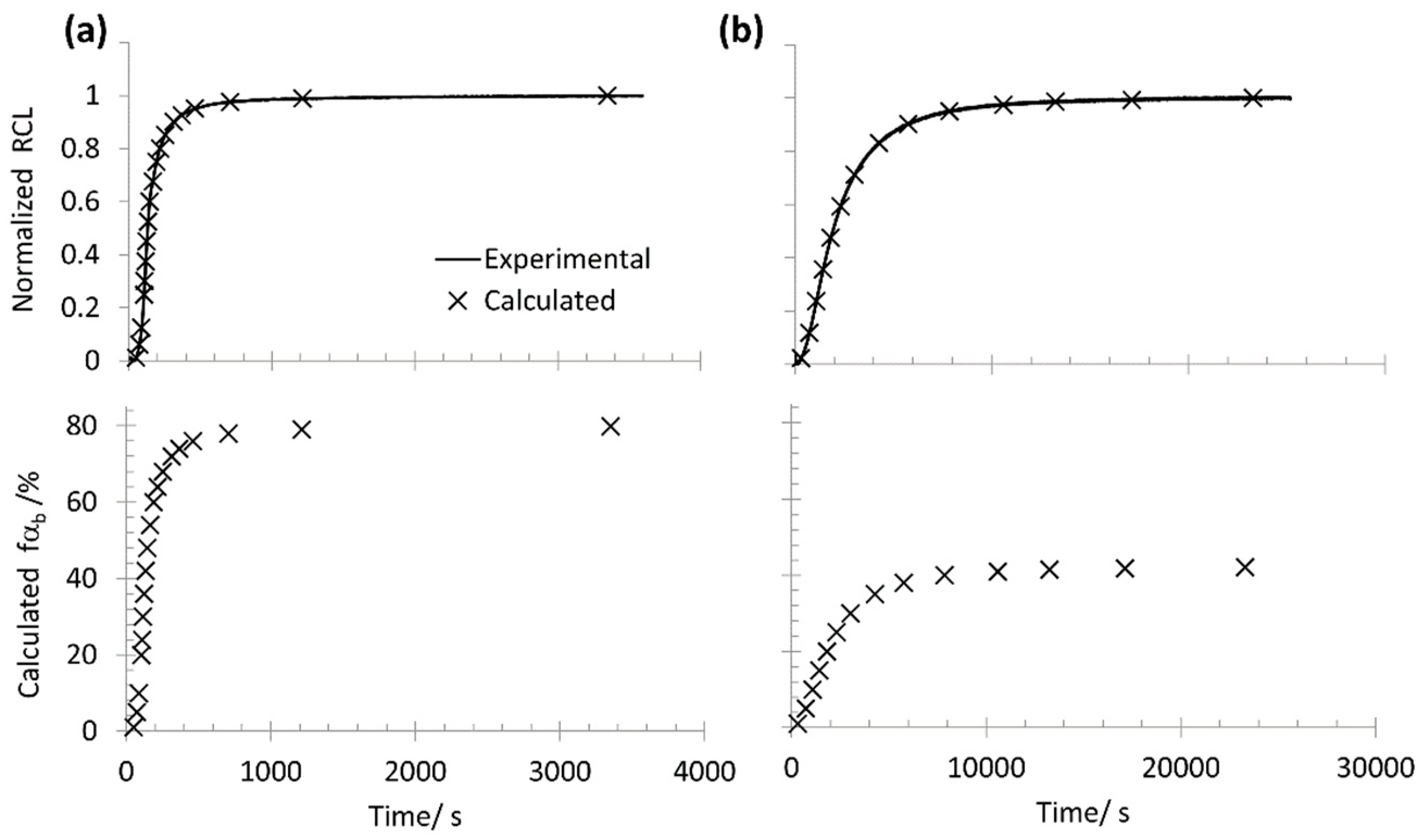
3.3. Method II. Dilatometric Curve Simulation by Atomic Volumes

In this method, a combination of some experimental data, dilatometry of the longest experiment in Region 3 and its XRD analysis, together with atomic volume calculations, are used in an attempt to simulate the RCL curve and, in turn, the ${\mathrm{f}}_{{\mathsf{\alpha }}_{\mathrm{b}}}$ vs. time, from where an estimation of the EBT can be made [44,45,46]. The principles of the method are as follows.

At constant temperature, any change in the RCL curve must be associated with a phase transformation. The density change resulting from the appearance of a new phase, with a different lattice parameter and unit cell, leads to a change in the total length of the sample. Considering bainitic transformation as isotropic, it is possible to calculate the dilatation associated to the transformation based on atomic volumes. Under such an assumption, the relative change in volume $\left(\Delta \mathrm{V}/{\mathrm{V}}_0\right)$ is related to the relative change in length $\left(\Delta \mathrm{L}/{\mathrm{L}}_0\right)$ as follows:

$$\frac{\Delta \mathrm{V}}{{\mathrm{V}}_0}=\frac{{\mathrm{V}}_{\mathrm{f}}-{\mathrm{V}}_0}{{\mathrm{V}}_0}=\frac{{\left({\mathrm{L}}_0+\Delta \mathrm{L}\right)}^3-{\mathrm{L}}_0^3}{{\mathrm{L}}_0^3}\cong 3\frac{\Delta \mathrm{L}}{{\mathrm{L}}_0}$$

(1)

where $\mathrm{L}$ and $\mathrm{V}$ stand for the length and volume of the sample and the subscript 0 and f for initial and final state, respectively.

The term $\Delta \mathrm{L}/{\mathrm{L}}_0$ is directly obtained from dilatometry curves, while the term $\Delta \mathrm{V}/{\mathrm{V}}_0$ can be obtained through the specific volumes and the amount of the different phases in the microstructure for the initial and final state. In this way, the initial and final volume for the bainite transformation can be obtained using the following expressions:

$${\mathrm{V}}_{\mathrm{f}}={\mathrm{f}}_{{\mathsf{\gamma }}^{+}}{\mathrm{V}}_{{\mathsf{\gamma }}^{+}}+{\mathrm{f}}_{{\mathsf{\alpha }}_{\mathrm{b}}}{\mathrm{V}}_{{\mathsf{\alpha }}_{\mathrm{b}}}$$

(2)

$${\mathrm{V}}_0={\mathrm{f}}_{\mathsf{\gamma }}{\mathrm{V}}_{\mathsf{\gamma }}$$

(3)

where fi is the fraction and ${\mathrm{V}}_{\mathrm{i}}$ is the specific volume of the corresponding phases, i.e., initial austenite ($\mathsf{\gamma }$), bainitic ferrite $({\mathsf{\alpha }}_b$), and C enriched retained austenite $({\mathsf{\gamma }}^{+})$. The corresponding atomic volumes (${\mathrm{V}}_{{\mathsf{\gamma }}^{+}}$,${\mathrm{V}}_{\mathsf{\alpha }}$, and ${\mathrm{V}}_{\mathsf{\gamma }}$), can be calculated from the different lattice parameters obtained from XRD experiments, see

Table 2. Lattice parameters for austenite (a_γ) and bainitic ferrite (a_α and c_α) obtained from XRD experiments.

Alloy	TIso/°C	aγ/Å	aα/Å	cα/Å
Steel 1	300	3.612	2.852	2.876
	325	3.614	2.853	2.875
	350	3.609	2.854	2.877
Steel 2	250	3.627	2.852	2.877
	300	3.626	2.850	2.876
	350	3.621	2.854	2.874

, following the expressions shown in

Table 3. Specific atomic volume, ${\mathrm{V}}_{\mathrm{i}}$, and thermal expansion coefficients, ${\mathrm{e}}_{\mathrm{i}}$, of the different unit cells used in this work, i. Their corresponding lattice parameters are denoted by a_i, and c_i. T stands for the temperature in °C.

Phase (i)	${\mathbf{V}}_{\mathbf{i}}$	${\mathbf{e}}_{\mathbf{i}}/°{\mathbf{C}}^{-1}$
fcc (γ)	$\frac{{\mathrm{a}}_{\mathrm{i}}^3}{4}$	2.065 × 10−5 [21]
bct (a)	$\frac{{\mathrm{a}}_{\mathrm{i}}^2\mathrm{c}}{2}$	1.490 × 10−5 [51]

[33,47]. The fractions ${\mathrm{f}}_{{\mathsf{\gamma }}^{+}}{\mathrm{and}\mathrm{f}}_{{\mathsf{\alpha }}_{\mathrm{b}}}$ are those also obtained by XRD, while ${\mathrm{f}}_{\mathsf{\gamma }}=100\%$, as bainitic ferrite will start to form from a fully austenitic microstructure. It is necessary to remark that in the context of low temperature bainite, the carbon that persists in solid solution within the bainitic ferrite, even after extended heat treatments, is sufficiently Zener ordered to cause the bainitic ferrite unit cell to be noncubic but tetragonal [30,48,49,50].

The lattice parameter of a certain phase at a given temperature, ${\mathrm{a}}_{\mathrm{i}}\left({\mathrm{T}}_{\mathrm{Iso}}\right)$, correlates with that obtained at room temperature from X-ray experiments, ${\mathrm{a}}_{\mathrm{i}}\left(25°\mathrm{C}\right)$, following expressions of the type:

$${\mathrm{a}}_{\mathrm{i}}\left({\mathrm{T}}_{\mathrm{Iso}}\right)={\mathrm{a}}_{\mathrm{i}}\left(25°\mathrm{C}\right)\left(1+{\mathrm{e}}_{\mathrm{i}}\left({\mathrm{T}}_{\mathrm{Iso}}-25\right)\right),$$

(4)

where ${\mathrm{e}}_{\mathrm{i}}$ is the thermal expansion coefficient, and the specific values used in this work are shown in Table 3 [21,51].

Therefore, the relative change in length at a certain isothermal temperature can be calculated using the lattice parameters and the equations above mentioned as:

$$\frac{\Delta \mathrm{L}}{{\mathrm{L}}_0}=\frac{1}{3}\left[\frac{\left(2{\mathrm{f}}_{{\mathsf{\alpha }}_{\mathrm{b}}}{\mathrm{a}}_{{\mathsf{\alpha }}_{\mathrm{b}}}{}^2{\mathrm{c}}_{{\mathsf{\alpha }}_{\mathrm{b}}}+{\mathrm{f}}_{{\mathsf{\gamma }}^{+}}{\mathrm{a}}_{{\mathsf{\gamma }}^{+}}^3\right)-{\mathrm{a}}_{\mathsf{\gamma }}^3}{{\mathrm{a}}_{\mathsf{\gamma }}^3}\right].$$

(5)

The following steps are described below:

• From XRD data, bainitic ferrite fraction $({\mathrm{f}}_{{\mathsf{\alpha }}_{\mathrm{b}}})$ and lattice parameters, ${\mathrm{a}}_{{\mathsf{\alpha }}_{\mathrm{b}}}$ and ${\mathrm{c}}_{{\mathsf{\alpha }}_{\mathrm{b}}}$, are calculated from the lattice parameters, and its C content (${\mathrm{C}}_{\mathsf{\alpha }}$) is derived using [52]. It has been proven that bainitic ferrite is fairly stable through the whole transformation regardless of the degree of transformation, and therefore, ${\mathrm{a}}_{{\mathsf{\alpha }}_{\mathrm{b}}}$ and ${\mathrm{c}}_{{\mathsf{\alpha }}_{\mathrm{b}}}$, i.e., ${\mathrm{C}}_{\mathsf{\alpha }}$, will remain constant from the beginning to the end of the transformation [24].
• For ${\mathrm{f}}_{{\mathsf{\alpha }}_{\mathrm{b}}}$ = 1%, the lever rule is applied ${\mathrm{C}}_{bulk}={\mathrm{f}}_{{\mathsf{\gamma }}^{+}}{\mathrm{C}}_{{\mathsf{\gamma }}^{+}}+{\mathrm{f}}_{{\mathsf{\alpha }}_{\mathrm{b}}}{C}_{{\alpha }_b}$ to calculate ${\mathrm{C}}_{{\mathsf{\gamma }}^{+}}$ for that amount of transformed bainitic ferrite.
• From the obtained ${\mathrm{C}}_{{\mathsf{\gamma }}^{+}},$ a value of the corresponding lattice parameter ${\mathrm{a}}_{{\mathsf{\gamma }}^{+}}^{}$ is derived using the expression given in [33,53].
• With all that information, and using Equation (4), the lattice parameters at the studied temperature are calculated. Then, Equation (5) is used to calculate ${\left(\Delta \mathrm{L}/{\mathrm{L}}_0\right)}_{1\%}$, associated with the formation of 1% of bainitic ferrite.
• The process is repeated for different values of ${\mathrm{f}}_{{\mathsf{\alpha }}_{\mathrm{b}}}$ up to the fraction provided by the XRD experiment, ${\mathrm{f}}_{{\mathsf{\alpha }}_{\mathrm{b}}}={\mathrm{f}}_{{\mathrm{XRD}}_{}}$.

Up to this point, we have managed to correlate a value of ${\mathrm{f}}_{{\mathsf{\alpha }}_{\mathrm{b}}}$ with its corresponding ${\left(\Delta \mathrm{L}/{\mathrm{L}}_0\right)}_{{\mathrm{f}}_{{\mathsf{\alpha }}_{\mathrm{b}}}}$, but it is necessary to establish at what time, on the experimental dilatometry curve, such events occur. However, there are certain drawbacks that must be considered.

First, as the time for a calculated ${\left(\Delta \mathrm{L}/{\mathrm{L}}_0\right)}_{{\mathrm{f}}_{{\mathsf{\alpha }}_{\mathrm{b}}}}$ has to be identified in the experimental curve, this method still depends to some extent on whether the dilatometric curve reaches horizontality or not. Second, by using the lever rule to calculate ${\mathrm{C}}_{{\mathsf{\gamma }}^{+}}$, a greater supersaturation in C is being assigned to austenite. In other words, all the C that is not in bainitic ferrite is assigned to the parent austenite (${\mathsf{\gamma }}^{+})$, but it is extensively reported that there is a large amount of that carbon distributed between dislocations as Cottrell atmospheres, in C clusters, and also as nanoprecipitates [54,55,56]. To illustrate the great differences between the estimated ${\mathrm{C}}_{{\mathsf{\gamma }}^{+}}$ from the lever rule and from XRD, serve as an example Steel 1 at 250 °C, according to the former ${\mathrm{C}}_{{\mathsf{\gamma }}^{+}}$ = 2.4 wt.%, which is much higher than that based on the lattice parameter obtained by XRD, ${\mathrm{C}}_{{\mathsf{\gamma }}^{+}}$ = 1.4 wt.%. Such a difference has an important effect in the ${\left(\Delta \mathrm{L}/{\mathrm{L}}_0\right)}_{{\mathrm{f}}_{{\mathsf{\alpha }}_{\mathrm{b}}}}$ calculations as they rely on estimated lattice parameters. Finally, the theoretical calculations take into account neither the influence of dislocation density, introduced during the transformation [45], nor the internal stresses introduced during cooling to room temperature in the microstructure, as a consequence of the different thermal expansion coefficients of austenite and bainitic ferrite [37].

For all those reasons, normalization, to the maximum of the experimental and calculated $\left(\Delta \mathrm{L}/{\mathrm{L}}_0\right)$ curves, has proven to minimize such disagreements. Therefore:

• The newly obtained results are then normalized, as it is also the experimental $\left(\Delta \mathrm{L}/{\mathrm{L}}_0 \right)$ curve.
• From the normalized ${\left(\Delta \mathrm{L}/{\mathrm{L}}_0\right)}_{{\mathrm{f}}_{{\mathsf{\alpha }}_{\mathrm{b}}}}$, a match is found in the—also normalized—dilatometric curve, and therefore, its corresponding experimental time is established.

A couple of examples illustrating the type of calculations just described are shown in Figure 6. For comparative purposes, the experimental and calculated normalized RCL are presented together with the evolution of the calculated ${\mathrm{f}}_{{\mathsf{\alpha }}_{\mathrm{b}}}$; note that the last values correspond to that also measured by XRD, ${\mathrm{f}}_{{\mathsf{\alpha }}_{\mathrm{b}}}= {\mathrm{f}}_{{\mathrm{XRD}}_{}}$.

• Finally, the EBT time would be that at which the calculated ${\mathrm{f}}_{{\mathsf{\alpha }}_{\mathrm{b}}}={\mathrm{f}}_{\mathrm{XRD}}$, but a less conservative value will be obtained allowing for the XRD uncertainty (±3%), so the EBT can also be calculated as that at which ${\mathrm{f}}_{{\mathsf{\alpha }}_{\mathrm{b}}}={\mathrm{f}}_{\mathrm{XRD}}$ − 1% or that when ${\mathrm{f}}_{{\mathsf{\alpha }}_{\mathrm{b}}}={\mathrm{f}}_{\mathrm{XRD}}$ − 2%.

In addition to those already mentioned, some other drawbacks of the method are the amount of time consuming calculations, the consequent assumptions, and other intermediate formulas and parameters whose expressions and values are not constant through the literature (as lattice parameter as a function of chemical composition or the values of thermal expansion coefficients), but also the need of performing XRD experiments.

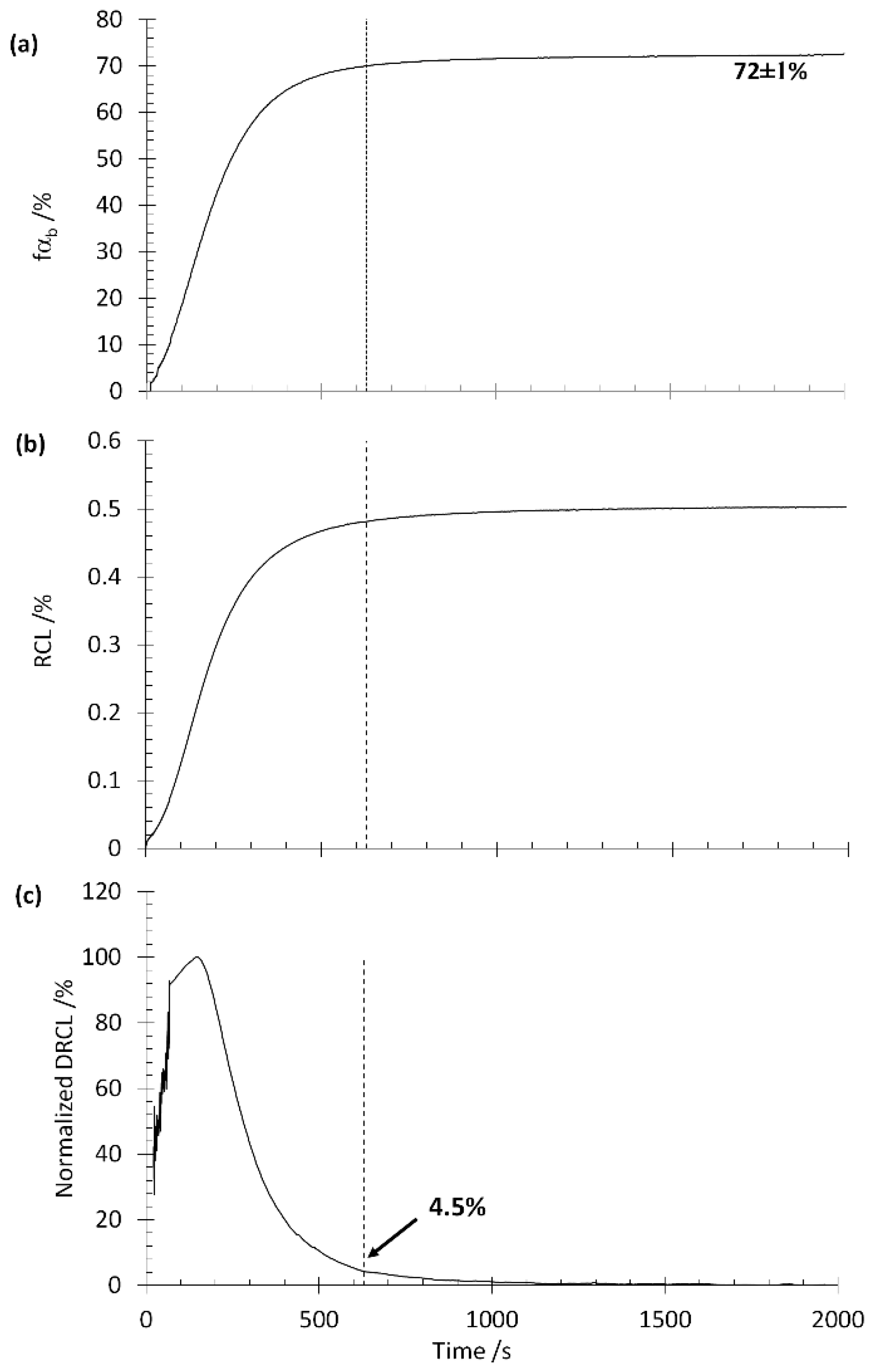
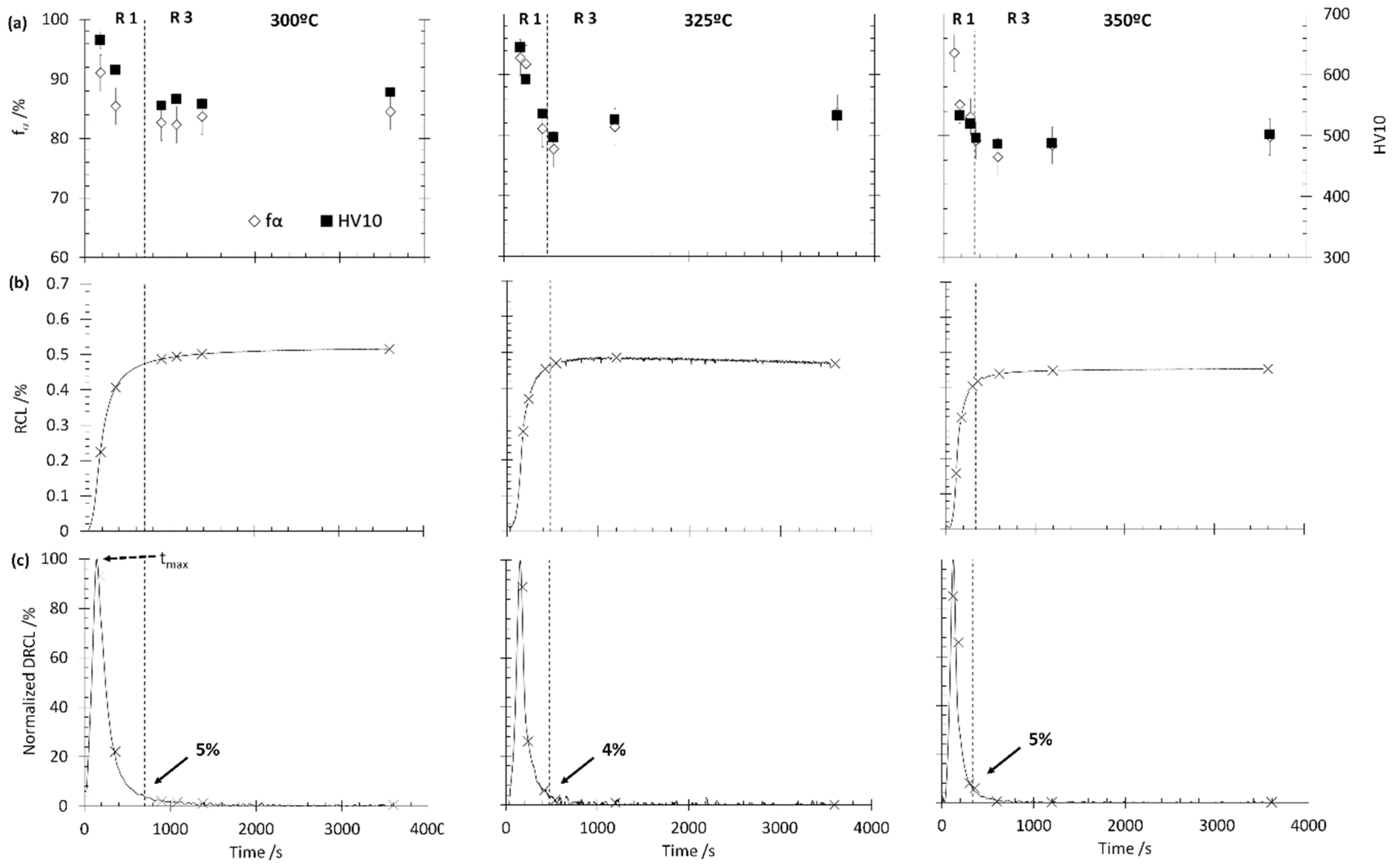
3.4. Method III. Rate of Transformation Approach

Method III only relies on high-resolution dilatometer data, which makes it simple and straightforward to apply.

From the sigmoidal curve obtained for any bainitic transformation, the transformation rate can be studied through the first derivative of the RCL (DRCL), see Figure 2c and Figure 3c. After the initial incubation period, the transformation rate increases dramatically, and after a maximum (at a time t_max), the transformation becomes slower and very sluggish for the latter stages of transformation. It is important to note that, as the maximum transformation rate occurs relatively early in the experiment, t_max is independent of both the exact duration of the test and also whether the asymptotic line at the end of the curve is actually reached or not.

In this method, the proposal for a simple, reproducible, and objective estimation of the EBT time is based on finding above which percentage of the maximum rate of transformation we are certainly operating in Region 3. Again, normalizing the DRCL, Figure 2c and Figure 3c, helps for a better comparison of the curves for both steels, as otherwise, the difference in the values of the DRCL, due to the differences in the transformation kinetics between Steel 1 and Steel 2, is of two orders of magnitude. For faster transformation kinetics, the DRCL shows a very steep increase and decrease after the maximum, narrow peak, while in slower transformations, the peak is much wider.

According to the adopted definition of Region 3, it is safe to assume that the EBT time can be defined above the percentage where the DRCL and Region 3 intersect, indicated by arrows in Figure 2c and Figure 3c. As can be seen in these same figures, for Steel 1, such a percentage is in all cases ≤4%, while for Steel 2, it is ≤11%. Therefore, what is for certain is that, being conservative, we can define 4% of the maximum of the transformation rate as a threshold to assume that the transformation is certainly finished. It has to be regarded that due to the data-noise created by the derivative in DRCL, if a very small % of the maximum is selected, a clear definition of the EBT might become difficult. This difficulty can be overcome by simply reducing the amount of data acquired during the isothermal step or by cleaning the post-experiment data, always respecting the shape of the first derivative.

A summary of the EBT time obtained by the different methods is shown in

Table 4. Summary of results of the EBT (in s) obtained by the different methods discussed in this paper. The results obtained according to Method 0 are an approximation for the shortest time from where there is no more bainitic transformation detectable by means of XRD and HV measurements, i.e., beginning of Region 3. DRCL stands for the derivative of the relative change in length.

Alloy	TIso (°C)	Method 0	Method I	EBT/s
				Method II $\mathbf{X}\%={\mathbf{f}}_{\mathbf{X}\mathbf{R}\mathbf{D}}-{\mathbf{f}}_{{\mathsf{\alpha }}_{\mathbf{b}}}$			Method III % of the Maximum DRCL
				0%	1%	2%	4%	3%	2%
Steel 1	300	700	1700	3600	1252	1123	694	777	932
	325	470	500	3596	3596	3596	480	490	530
	350	340	1100	3347	1213	705	378	406	475
Steel 2	250	21,000	42,014	50,274	37,050	27,581	25,458	-	-
	300	6500	12,500	28,764	15,004	11,455	8020	8690	-
	350	5200	11,000	23,284	10,599	7859	7503	8032	-
Steel 3	400	630	1264	1988	870	688	653	724	818

. Note that results obtained according to Method 0 are an approximation for the shortest time from where there is no more bainitic transformation detectable by means of XRD and HV measurements, i.e., beginning of Region 3. Therefore, in order to consider a result as viable, it has to be equal or greater than that value. Data have to be consistent also in reflecting that the transformation is slower as the isothermal transformation is lowered, or the C content increased.

From the obtained results, it is clear that Method I does not always provide a viable estimation of the EBT—see, for example, Steel 1 and the increase of the EBT calculated from 325 to 350 °C. Further, when it is possible to determine EBT, it is usually well into Region 3, which leads to overestimation. Keep in mind that the results might change if a different operator tries to estimate the time.

In the case of Method II, the EBT was calculated, as anticipated, for three different scenarios, X = 0%, 1% and 2%, where X = ${\mathrm{f}}_{\mathrm{XRD}}-{\mathrm{f}}_{{\mathsf{\alpha }}_{\mathrm{b}}}$. It was possible to obtain a coherent EBT in most of the cases, except for the Steel 1 at 325 °C where the continuous decrease of the dilatometric curve in Region 3 made the three calculated EBT identical and equal to the total duration of the experiment. In the other cases, note as well that for the variant X = 0%, the EBT values are also close to the duration of the isothermal heat treatment, again, a problem associated with deviation from a horizontal line in Region 3. On the other hand, results from the X = 1 and 2% provided much shorter EBT times and all within Region 3. The results of the method are also consistent in the sense that EBT tends to decrease as the percentage allowed to deviate from ${\mathrm{f}}_{\mathrm{XRD}}$ decreases.

As for Method III, several percentages of the maximum DRCL were tested, i.e., 4%, 3%, and 2%. In the case of the 4% it was possible the determination of the EBT for all steels and tested temperatures. As anticipated, when the percentage selected was smaller, as in the case of the 3% and 2%, the time increased, and its determination was not possible in all cases, for example, Steel 2, as there were several possible solutions due to data-noise introduced by the derivative.

Note that differences in the reported EBT times could lead to reductions of the treatment in the range of minutes to almost 7 h.

A final validation of the 4% criteria was done using data provided by an in situ high energy X-ray diffraction (HEXRD) facility fitted with a dilatometer, which allows for the simultaneous tracking of dilatation and the phase evolution during bainitic transformation. The experiment was performed in Steel 3, and the heat treatment parameters used to obtain a bainitic microstructure were T_γ = 900 °C, T_Iso = 400 °C and t_iso = 2000 s; note that the experimental Ms is 320 °C. The results obtained are summarized in Figure 7. Unlike the experiments conducted in Steel 1 and Steel 2, in this case, the evolution of the bainitic ferrite fraction was recorded during the whole extension of the isothermal test, reaching a maximum and steady value of ${\mathrm{f}}_{{\mathsf{\alpha }}_{\mathrm{b}}}$ = 72 ± 1%. The progressive increase of ${\mathrm{f}}_{{\mathsf{\alpha }}_{\mathrm{b}}}$ as a sigmoidal type curve has, as expected, its reflection in the dilatometry curve, both being identical curves, see Figure 7a,b. For Steel 3, only the beginning of Region 3 can be defined, which was set as the time when ${\mathrm{f}}_{{\mathsf{\alpha }}_{\mathrm{b}}}$= 70%, represented by the dotted line in Figure 7 and shown in Figure 7c to correspond to 4.5% of the maximum DRCL, Method 0 in Table 4. The other methods discussed in this work were also tested, and the results are listed in Table 3. These results, and their trends, are in line with those obtained for Steel 1 and Steel 2. The EBT time calculated by means of Method I was overestimated, whereas in the case of Method II, the EBT value was closer to that determined by Method 0 as the percentage X% ($={\mathrm{f}}_{\mathrm{XRD}}-{\mathrm{f}}_{{\mathsf{\alpha }}_{\mathrm{b}}})$ increases. Finally, in Method III, it is clear that EBT calculated using the 4% of the maximum DRLC is very similar to that of Method 0, thus validating the selection of this percentage as a threshold for the determination of the EBT.

In view of the results obtained in the three steels studied, of very different chemical compositions and bainitic transformation kinetics, it seems clear that 4% of the maximum of the DRCL, Method III, is well within Region 3 or delimiting its start. Therefore, when the determination of EBT is required either with purely scientific objectives or for the definition of an industrial process, and taking into account the limitations listed above, it should be done with percentages of the maximum DRCL ≤ 4%.

4. Conclusions

In this work, we revised some of the most common methods used to establish the end of bainitic transformation (EBT). The advantages and disadvantages of each have been analyzed, taking into account the number and type of added experiments required, time consumption, level of uncertainty and difficulty, operator intervention (subjectivity), etc.

After comparing and validating the results, it was concluded that the method based on the derivative of the relative change in length is, by far, the simplest, most operator-independent, most accurate and reliable of all of them.

If this method is adopted, the comparison of the results obtained between the different laboratories and those in which different measures are adopted to try to alter the kinetics of the bainitic transformation will have a greater meaning and be more objective. In the same way, we believe that the widespread belief regarding the need for excessively long treatments for the development of low temperature bainite will dissipate.

References

1. Christian, J.W.; Olson, G.B.; Cohen, M. Classification of displacive transformations: What is a martensitic transformation? J. Phys. IV Colloq. 1995, 05, C8-3–C8-10. [Google Scholar] [CrossRef]
2. Bhadeshia, H.K.D.H. Bainite in Steels: Transformations, Microstructure and Properties, 3rd ed.; Institute of Materials, Minerals and Mining: London, UK, 2015. [Google Scholar]
3. Bhadeshia, H.K.D.H. Bainite in Steels: Theory and Practice, 3rd ed.; Maney Publishing: Leeds, UK, 2015; p. 616. [Google Scholar]
4. Bhadeshia, H.K.D.H.; Honeycombe, R.W.K. Steels: Microstructure and Properties; Butterworths-Heinemann (Elsevier): Oxford, UK, 2006. [Google Scholar]
5. Caballero, F.G.; Morales-Rivas, L.; Garcia-Mateo, C. Retained austenite: Stability in a nanostructured bainitic steel. In Encyclopedia of Iron, Steel, and Their Alloys; Taylor & Francis: Abingdon-on-Thames, UK, 2016; pp. 3077–3087. [Google Scholar]
6. Garcia-Mateo, C.; Caballero, F.G.; Miller, M.K.; Jimenez, J.A. On measurement of carbon content in retained austenite in a nanostructured bainitic steel. J. Mater. Sci. 2012, 47, 1004–1010. [Google Scholar] [CrossRef]
7. Garcia-Mateo, C.; Caballero, F.G. Ultra-high-strength bainitic steels. ISIJ Int. 2005, 45, 1736–1740. [Google Scholar] [CrossRef]
8. Garcia-Mateo, C.; Caballero, F.G. Understanding the mechanical properties of nanostructured bainite. In Handbook of Mechanical Nanostructuring; Aliofkhazraei, M., Ed.; Wiley: Weinheim, Germany, 2015; Volume 1, pp. 35–65. [Google Scholar]
9. Rakha, K.; Beladi, H.; Timokhina, I.; Xiong, X.; Kabra, S.; Liss, K.D.; Hodgson, P. On low temperature bainite transformation characteristics using in-situ neutron diffraction and atom probe tomography. Mater. Sci. Eng. A 2014, 589, 303–309. [Google Scholar] [CrossRef]
10. Xing, X.L.; Yuan, X.M.; Zhou, Y.F.; Qi, X.W.; Lu, X.; Xing, T.H.; Ren, X.J.; Yang, Q.X. Effect of bainite layer by lsmcit on wear resistance of medium-carbon bainite steel at different temperatures. Surf. Coat. Technol. 2017, 325, 462–472. [Google Scholar] [CrossRef]
11. Zhang, M.; Wang, T.S.; Wang, Y.H.; Yang, J.; Zhang, F.C. Preparation of nanostructured bainite in medium-carbon alloysteel. Mater. Sci. Eng. A 2013, 568, 123–126. [Google Scholar] [CrossRef]
12. Hu, F.; Wu, K.M.; Wan, X.L.; Rodionova, I.; Shirzadi, A.A.; Zhang, F.C. Novel method for refinement of retained austenite in micro/nano-structured bainitic steels. Mater. Sci. Technol. 2017, 33, 1360–1365. [Google Scholar] [CrossRef] [Green Version]
13. Zhao, J.; Hou, C.S.; Zhao, G.; Zhao, T.; Zhang, F.C.; Wang, T.S. Microstructures and mechanical properties of bearing steels modified for preparing nanostructured bainite. J. Mater. Eng. Perform. 2016, 25, 4249–4255. [Google Scholar] [CrossRef]
14. Nishijima, H.; Tomota, Y.; Su, Y.; Gong, W.; Suzuki, J.I. Monitoring of bainite transformation using in situ neutron scattering. Metals 2016, 6, 16. [Google Scholar] [CrossRef]
15. Kabirmohammadi, M.; Avishan, B.; Yazdani, S. Transformation kinetics and microstructural features in low-temperature bainite after ausforming process. Mater. Chem. Phys. 2016, 184, 306–317. [Google Scholar] [CrossRef]
16. Jiang, T.; Liu, H.; Sun, J.; Guo, S.; Liu, Y. Effect of austenite grain size on transformation of nanobainite and its mechanical properties. Mater. Sci. Eng. A 2016, 666, 207–213. [Google Scholar] [CrossRef]
17. Yakubtsov, I.A.; Purdy, G.R. Analyses of transformation kinetics of carbide-free bainite above and below the athermal martensite-start temperature. Metall. Mater. Trans. A 2011, 43, 437–446. [Google Scholar] [CrossRef]
18. Garcia-Mateo, C.; Caballero, F.G. Nanocrystalline bainitic steels for industrial applications. In Nanotechnology for Energy Sustainability; Wiley-VCH Verlag GmbH & Co. KGaA: Weinheim, Germany, 2017; pp. 707–724. [Google Scholar]
19. Garcia-Mateo, C.; Caballero, F.G.; Bhadeshia, H.K.D.H. Acceleration of low-temperature bainite. ISIJ Int. 2003, 43, 1821–1825. [Google Scholar] [CrossRef]
20. Eres-Castellanos, A.; Morales-Rivas, L.; Latz, A.; Caballero, F.G.; Garcia-Mateo, C. Effect of ausforming on the anisotropy of low temperature bainitic transformation. Mater. Charact. 2018, 145, 371–380. [Google Scholar] [CrossRef]
21. Saha Podder, A.; Bhadeshia, H.K.D.H. Thermal stability of austenite retained in bainitic steels. Mater. Sci. Eng. A 2010, 527, 2121–2128. [Google Scholar] [CrossRef] [Green Version]
22. Morales-Rivas, L.; Yen, H.W.; Huang, B.M.; Kuntz, M.; Caballero, F.G.; Yang, J.R.; Garcia-Mateo, C. Tensile response of two nanoscale bainite composite-like structures. JOM 2015, 67, 2223–2235. [Google Scholar] [CrossRef]
23. Avishan, B.; Garcia-Mateo, C.; Yazdani, S.; Caballero, F.G. Retained austenite thermal stability in a nanostructured bainitic steel. Mater. Charact. 2013, 81, 105–110. [Google Scholar] [CrossRef] [Green Version]
24. Rementeria, R.; Jimenez, J.A.; Allain, S.Y.P.; Geandier, G.; Poplawsky, J.D.; Guo, W.; Urones-Garrote, E.; Garcia-Mateo, C.; Caballero, F.G. Quantitative assessment of carbon allocation anomalies in low temperature bainite. Acta Mater. 2017, 133, 333–345. [Google Scholar] [CrossRef]
25. Sourmail, T.; Smanio, V. Determination of ms temperature: Methods, meaning and influence of ‘slow start’ phenomenon. Mater. Sci. Technol. 2013, 29, 883–888. [Google Scholar] [CrossRef]
26. Sourmail, T.; Smanio, V.; Ziegler, C.; Heuer, V.; Kuntz, M.; Caballero, F.G.; Garcia-Mateo, C.; Cornide, J.; Elvira, R.; Leiro, A.; et al. Novel Nanostructured Bainitic Steel Grades to Answer the Need for High-Performance Steel Components (Nanobain); European Commission: Luxembourg, 2013; p. 129. [Google Scholar]
27. Garcia-Mateo, C.; Sourmail, T.; Caballero, F.G.; Smanio, V.; Kuntz, M.; Ziegler, C.; Leiro, A.; Vuorinen, E.; Elvira, R.; Teeri, T. Nanostructured steel industrialisation: Plausible reality. Mater. Sci. Technol. 2014, 30, 1071–1078. [Google Scholar] [CrossRef]
28. Bhadeshia, H.K.D.H. Thermodynamic analysis of isothermal transformation diagrams. Met. Sci. 1982, 16, 159–165. [Google Scholar] [CrossRef]
29. Caballero, F.G.; Garcia-Mateo, C.; de Andres, C.G. Dilatometric study of reaustenitisation of high silicon bainitic steels: Decomposition of retained austenite. Mater. Trans. JIM 2005, 46, 581–586. [Google Scholar] [CrossRef]
30. Garcia-Mateo, C.; Jimenez, J.A.; Yen, H.W.; Miller, M.K.; Morales-Rivas, L.; Kuntz, M.; Ringer, S.P.; Yang, J.R.; Caballero, F.G. Low temperature bainitic ferrite: Evidence of carbon super-saturation and tetragonality. Acta Mater. 2015, 91, 162–173. [Google Scholar] [CrossRef] [Green Version]
31. ASTM International. Standard Practice for X-Ray Determination of Retained Austenite in Steel with Near Random Crystallographic Orientation; ASTM International: West Conshohocken, PA, USA, 2013; Volume ASTM E975-13, p. 7. [Google Scholar]
32. Jarvinen, M. Texture effect in x-ray analysis of retained austenite in steels. Text. Microstruct. 1996, 26–27, 93–101. [Google Scholar] [CrossRef]
33. Dyson, D.J.; Holmes, B. Effect of alloying additions on lattice parameter of austenite. J. Iron Steel Inst. 1970, 208, 469–474. [Google Scholar]
34. Garcia-Mateo, C.; Caballero, F.G. The role of retained austenite on tensile properties of steels with bainitic microstructures. Mater. Trans. JIM 2005, 46, 1839–1846. [Google Scholar] [CrossRef]
35. Arnell, R.D.; Ridal, K.A.; Durnin, J. Determination of retained austenite in steel by x-ray diffraction. J. Iron Steel Inst. 1968, 206, 1035–1036. [Google Scholar]
36. Allain, S.Y.P.; Aoued, S.; Quintin-Poulon, A.; Goune, M.; Danoix, F.; Hell, J.C.; Bouzat, M.; Soler, M.; Geandier, G. In situ investigation of the iron carbide precipitation process in a Fe-C-Mn-Si Q&P steel. Materials 2018, 11, 1087. [Google Scholar]
37. Allain, S.Y.P.; Gaudez, S.; Geandier, G.; Hell, J.C.; Gouné, M.; Danoix, F.; Soler, M.; Aoued, S.; Poulon-Quintin, A. Internal stresses and carbon enrichment in austenite of quenching and partitioning steels from high energy x-ray diffraction experiments. Mater. Sci. Eng. A 2018, 710, 245–250. [Google Scholar] [CrossRef]
38. Garcia-Mateo, C.; Caballero, F.; Bhadeshia, H. Development of hard bainite. ISIJ Int. 2003, 43, 1238–1243. [Google Scholar] [CrossRef]
39. Garcia-Mateo, C.; Caballero, F.G.; Sourmail, T.; Kuntz, M.; Cornide, J.; Smanio, V.; Elvira, R. Tensile behaviour of a nanocrystalline bainitic steel containing 3 wt% silicon. Mater. Sci. Eng. A 2012, 549, 185–192. [Google Scholar] [CrossRef]
40. Cornide, J.; Garcia-Mateo, C.; Capdevila, C.; Caballero, F.G. An assessment of the contributing factors to the nanoscale structural refinement of advanced bainitic steels. J. Alloy. Compd. 2013, 577, S43–S47. [Google Scholar] [CrossRef]
41. Hehemann, R.F.; Troiano, A.R. Characteristics and Stabilization of the Bainite Reaction; Metal Hydrides Inc: Beverly, MA, USA, 1954. [Google Scholar]
42. Chong, S.H. Transformation and Toughness of Iron-9 Percent Nickel Alloy. Ph.D. Thesis, Sheffield Hallam University, Sheffield, UK, 1998. [Google Scholar]
43. Garcia-Mateo, C.; Caballero, F.G.; Sourmail, T.; Cornide, J.; Smanio, V.; Elvira, R. Composition design of nanocrystalline bainitic steels by diffusionless solid reaction. Met. Mater. Int. 2014, 20, 405–415. [Google Scholar] [CrossRef] [Green Version]
44. Xu, Y.; Xu, G.; Mao, X.; Zhao, G.; Bao, S. Method to evaluate the kinetics of bainite transformation in low-temperature nanobainitic steel using thermal dilatation curve analysis. Metals 2017, 7, 330. [Google Scholar] [CrossRef]
45. Garcia-Mateo, C.; Caballero, F.G.; Capdevila, C.; Garcia de Andres, C. Estimation of dislocation density in bainitic microstructures using high-resolution dilatometry. Scr. Mater. 2009, 61, 855–858. [Google Scholar] [CrossRef] [Green Version]
46. Santajuana, M.A.; Rementeria, R.; Kuntz, M.; Jimenez, J.A.; Caballero, F.G.; Garcia-Mateo, C. Low-temperature bainite: A thermal stability study. Metall. Mater. Trans. B 2018, 49, 2026–2036. [Google Scholar] [CrossRef]
47. Moyer, J.M.; Ansell, G.S. The volume expansion accompanying the martensite transformation in iron-carbon alloys. Metall. Trans. A 1975, 6, 1785. [Google Scholar] [CrossRef]
48. Hulme-Smith, C.N.; Peet, M.J.; Lonardelli, I.; Dippel, A.C.; Bhadeshia, H.K.D.H. Further evidence of tetragonality in bainitic ferrite. Mater. Sci. Technol. 2015, 31, 254–256. [Google Scholar] [CrossRef]
49. Bhadeshia, H.K.D.H. Carbon in cubic and tetragonal ferrite. Philos. Mag. 2013, 93, 3714–3725. [Google Scholar] [CrossRef]
50. Jang, J.H.; Bhadeshia, H.K.D.H.; Suh, D.W. Solubility of carbon in tetragonal ferrite in equilibrium with austenite. Scr. Mater. 2013, 68, 195–198. [Google Scholar] [CrossRef]
51. Lee, S.J.; Lusk, M.T.; Lee, Y.K. Conversional model of transformation strain to phase fraction in low alloy steels. Acta Mater. 2007, 55, 875–882. [Google Scholar] [CrossRef]
52. Cohen, M. The strengthening of steel. Trans. Metall. AIME 1962, 224, 638–657. [Google Scholar]
53. Garcia-Mateo, C.; Peet, M.; Caballero, F.G.; Bhadeshia, H.K.D.H. Tempering of hard mixture of bainitic ferrite and austenite. Mater. Sci. Technol. 2004, 20, 814–818. [Google Scholar] [CrossRef] [Green Version]
54. Rementeria, R.; Garcia-Mateo, C.; Caballero, F.G. New insights into carbon distribution in bainitic ferrite. HTM J. Heat Treat. Mater. 2018, 73, 68–79. [Google Scholar] [CrossRef]
55. Rementeria, R.; Capdevila, C.; Dominguez-Reyes, R.; Poplawsky, J.D.; Guo, W.; Urones-Garrote, E.; Garcia-Mateo, C.; Caballero, F.G. Carbon clustering in low-temperature bainite. Metall. Mater. Trans. A 2018, 49, 5277–5287. [Google Scholar] [CrossRef]
56. Rementeria, R.; Poplawsky, J.D.; Aranda, M.M.; Guo, W.; Jimenez, J.A.; Garcia-Mateo, C.; Caballero, F.G. Carbon concentration measurements by atom probe tomography in the ferritic phase of high-silicon steels. Acta Mater. 2017, 125, 359–368. [Google Scholar] [CrossRef] [Green Version]
Figure 1. (a) Scheme of the performed heat treatment, where H.R and C.R stand for heating and cooling rate, respectively, Bs and Ms for the bainite and martensite start temperatures, respectively, and α, γ, and θ for ferrite, austenite, and cementite, respectively. (b) Exemplified dilatometric signal, where the different stages and microstructures that can be obtained depending on the holding time can be seen. The regions delimited by R correspond to the four different regions that have been described in the main body of the text.
Metals 09 00925 g001
Figure 2. For Steel 1 treated at different isothermal temperatures and times, (a) experimental fraction of ferrite ( f α ) and Vickers hardness measurements (HV) as a function of time, (b) the relative change in length (RCL) from the dilatometry test, and (c) normalized derivative of the relative change in length (DRCL). The x symbols in (b,c) indicate the position of the interrupted tests whose f α and HV are also indicated in (a). Vertical dotted lines denote the limits of regions (R1 and R3) as described in the main body of the text and schematically shown in Figure 1. Note that region R2 is not detectable for Steel 1.
Metals 09 00925 g002
Figure 3. For Steel 2 treated at different isothermal temperatures and times, (a) experimental fraction of ferrite ( f α ) and HV as a function of time, (b) the relative change in length (RCL) from the dilatometry test, and (c) normalized derivative of the relative change in length (DRCL). The x symbols in (b,c) indicate the position of the interrupted tests whose f α and HV are also indicated in (a). Vertical dotted lines denote the limits of different regions (R1, R2 and R3) as described in the main body of the text and schematically shown in Figure 1. Note that region R2 is not detectable in all cases.
Metals 09 00925 g003
Figure 4. SEM images of the bainitic microstructure obtained after isothermal transformation at 300 °C in (a) Steel 1 and (b) Steel 2. The darker long slender features are the plates of bainitic ferrite ( α b ), and the lighter phase found as films and more blocky type features correspond to retained austenite (γ).
Metals 09 00925 g004
Figure 5. For Steel 1 treated at 350 °C, the relative change in length of two identical test leading to different dilatometric curves. Also marked is the end of the bainite transformation (EBT) obtained by means of Method I.
Metals 09 00925 g005
Figure 6. Illustrative example, for (a) Steel 1 and (b) Steel 2 treated at 350 °C, of the different outcomes of Method II, i.e., experimental normalized RCL compared to the calculated, and also the calculated fraction of bainitic ferrite ( f α b )   as a function of time.
Metals 09 00925 g006
Figure 7. For Steel 3, results from simultaneous in situ high energy X-ray diffraction (HEXRD) and dilatometry during isothermal bainitic transformation at 400 °C. (a) Experimental fraction of bainitic ferrite ( f α b )   as a function of time, (b) the relative change in length (RCL) from the dilatometry test, and (c) normalized derivative of the relative change in length (DRCL). The vertical dotted line denotes the limits of Region 3 as described in the main body of the text.
Metals 09 00925 g007