Effect of Grain Size and Density of Abrasive on Surface Roughness, Material Removal Rate and Acoustic Emission Signal in Rough Honing Processes

Abstract

Honing processes provide a special cross-hatch pattern to the internal surface of cylinders that favors oil flow. However, along honing operation the abrasive grains wear out and lose their ability to cut material. The honing chips mixed with oil fill the pores of the abrasives and they start cutting in an incorrect way, leading to clogging. In the present paper, honing experiments were carried out according to a 3² factorial design, with different grain size and density of abrasive grains. Roughness, material removal rate, and tool wear were determined. Acoustic emissions were also measured and the chirplet concept was applied in order to detect differences between correct and incorrect cutting operations. As a general trend roughness and material removal rate increase with grain size and with density of abrasive. However, when clogging occurs roughness and material removal rate decrease, because the abrasive grains tend to deform the material instead of cutting it. When the honing process is working appropriately, the chirplet diagram of the harmonic part of the signal shows constant marks. On the contrary, when it does not work properly, marks disappear with time and their frequencies decrease. The results of the present paper will allow monitoring the honing process in order to change the abrasives when they are not working properly.

1. Introduction

The honing process consists of removing material from the interior surfaces of cylinders by means of abrasive stones, with the aim of providing appropriate surface roughness. In the honing process, a honing head combines rotation movement with alternate linear movement in order to obtain a cross-hatch pattern with valleys that promote oil circulation for the lubrication of combustion engine cylinders during operation [1,2]. It is important to choose appropriate cutting conditions and abrasive features in order to ensure a correct cutting operation and the required surface topography [3]. The type of surface obtained is related to the tribological behavior of the cylinder liners [4].

As for surface finish, arithmetical mean height Ra is a common roughness parameter employed for the comparison of different machining processes [5]. Typical Ra values in honing processes range from 0.05 μm to 1.6 μm [6]. Parameters related to the Abbott–Firestone curve or bearing area curve (according to standard ISO 13565-2 [7]) are useful for assessing surfaces that will suffer wear during operation, such as cylinder internal surfaces. Parameter Rk or core roughness should be higher than parameters Rpk (reduced peak height) and Rvk (reduced valley depth), to assure the wear resistance of the internal surface. Rvk assures appropriate oil retention of valleys, heat dissipation, and space for the removed material. Mr1 monitors the part of the curve corresponding to small peaks and Mr2 monitors the part of the curve corresponding to valleys. After a running-in period, it is recommended that Rpk be lower than Rvk [8] to provide peakless surfaces with appropriate breaks in properties. This situation can also be achieved with the plateau honing operation, which removes peaks from previous honing operations. Typical values for parameters in combustion engines after plateau honing are Rpk ≤ 0.2 μm, Rk between 0.3 μm and 0.8 μm, and Rvk between 1.0 μm and 1.5 μm. Other requirements of the surface are that it must not show folded metal, cold working or must show uniformly cut grooves [9]. According to Davim, the most influential parameters on surface finish in honing operations are Rk and Mr2, with required values of 0.6–1.8 μm and 75–85% respectively. Rk ensures correct sliding between surfaces, while Mr2 provides the ability to retain lubrication oil [10]. After performing rough, semi- finish and plateau honing, el Mansori et al. reported higher Rk values up to 2.66 μm, Rpk values up to 0.82 μm, and Rvk values up to 2.21 μm. Mr1 values ranged between 3.61% and 7%, and Mr2 values between 82.8% and 86.3% [11].

Regarding material removal rate, Szabo reported values between 0.015 and 0.020 mm/s (0.090 and 0.120 cm/min) with cubic boron nitride (CBN) stones, and lower values between 0.012 and 0.015 mm/s (0.072 and 0.090 cm/min) with diamond stones [12]. Similar values were obtained by Vrac et al., between 0.015 and 0.021 mm/s (0.090 and 0.124 cm/min), in rough honing operations with diamond stones [13].

Analysis of the acoustic emission (AE) is a typical way to monitor proper operation in different machining processes, such as turning [14,15] or milling [16,17]. Analysis of the AE has the advantage that it provides underlying information that can help in making decisions in fault detection [18,19,20]. For example, grinding burn can be detected in grinding processes [21]. As for honing processes, Kanthababu et al. monitored AE for both fresh and worn out tools, and found that the main frequency of the signal depends on the cutting conditions [22]. Several methods are available for analyzing nonstationary or stationary signals with high non-deterministic components. Methods are based on time, frequency, or time-frequency domains [21]. However, the time domain does not provide the frequency description of the signals and vice versa. Thus, the time-frequency-scale (TFS) transform concept is needed in order to simultaneously and accurately solve the uncertain visualization of events, and their frequencies, occurring over time. Depending on the analysis approaches, time-frequency methods for feature extraction are classified into different groups [21]. The first group corresponds to time-frequency functions derived from translating, modulating and scaling a basis function. For example, the short-time Fourier transform (STFT) consists of gradually varying the window size used every time. It is a simple method to obtain a continuous volumetric representation of the signal as a function of time and frequency, and can be used in many applications [23,24]. Wavelet transform is another well-known TFS, in which a family of translates and dilates of one basic primitive mother wavelet is used as a piece of wave. As a result of this computational process it is possible to obtain smoothing of the Wigner distribution [25,26,27] from the spectrogram (time-frequency TF plane) to the scalogram (TS plane). The second group corresponds to Cohen’s class of bilinear time–frequency energy distributions: Wigner-Ville distribution, Margenau–Hill distribution and other [28]. The third group is based on rotation of the TF plane. It includes fractional Fourier transform, local polynomial Fourier transform, and Radon–Wigner distribution. The fourth group corresponds to signal dependent TFRs and includes concentration measures, reassignment methods, and signal optimized kernels/windows [21].

Chirplet transform is a more generalist method than wavelet because the mother pattern used is a single wave signal with a continuously variable frequency-amplitude between two limits as a piece of chirp, in concordance with a wavelet as a piece of wave [29]. Different authors have used chirplet for detecting failures, for example in gearboxes, on bearings [30,31], or gears [32]. Chirplet was also used for detecting weld defects [33]. Consequently, chirplet could be used in machining process monitoring. The honing process sound emissions are generated from a reciprocating tool movement and contain continuous frequency variations throughout. They have a similar shape to the chirp concept. For this reason, the sound analysis by means of the chirplet method could, in this case, be more advisable than other analysis methods.

The main aim of the present paper is to study and analyze the effect of grain size and density of abrasive grains on surface roughness, material removal rate, and tool wear in rough honing processes. For doing this, different rough honing experiments were carried out. In addition, AE signals of the experiments were measured. The signals were analyzed by means of chirplet transform and the observation of chirplet patterns. From the analysis, a methodology was developed to detect when the honing process is not performed correctly, for example because of clogging. The methodology will help to monitor honing and other machining processes in situ.

2. Materials and Methods

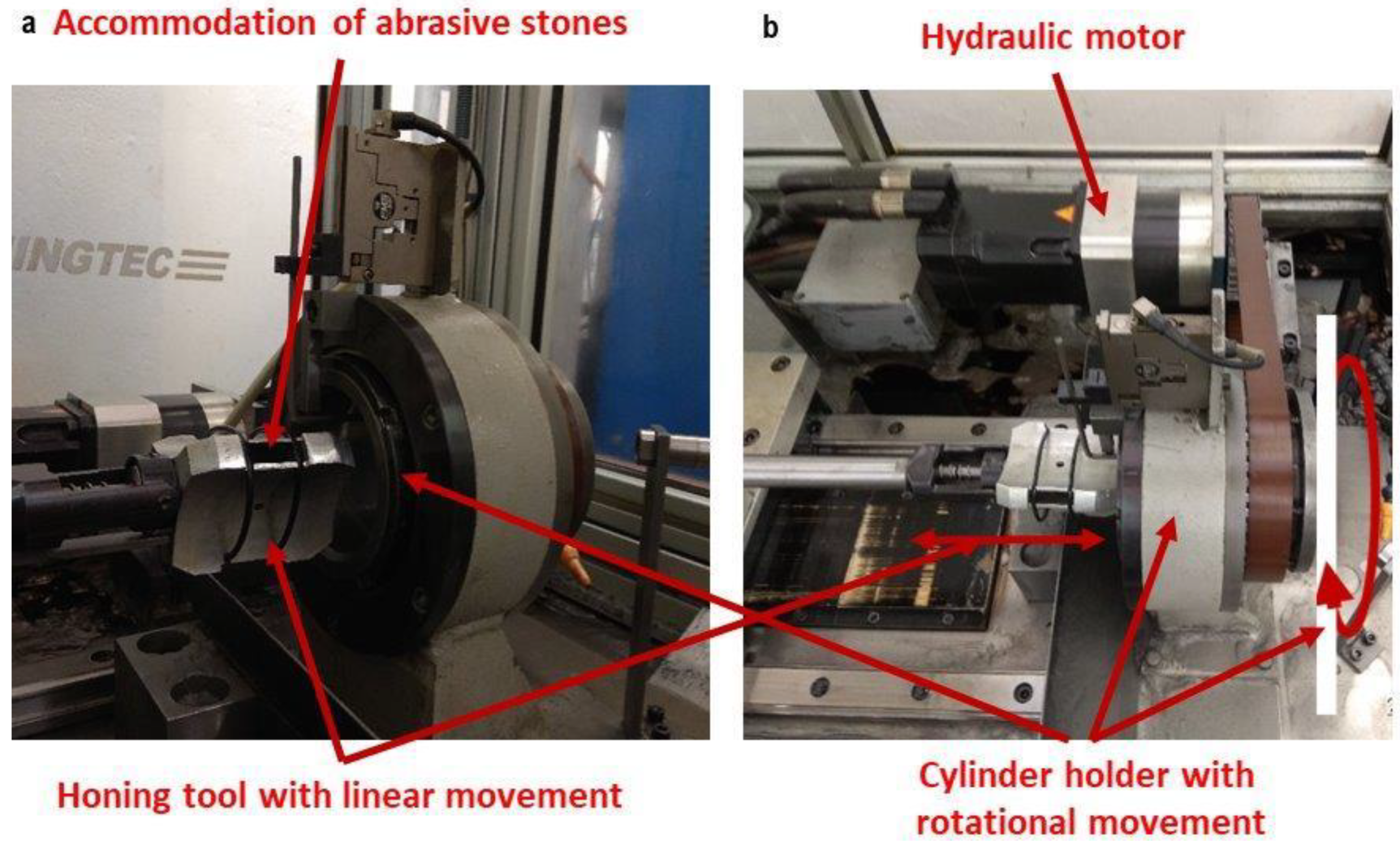
2.1. Honing Experiments

Steel St-52 (DIN 2391 [34]) cylinders of 80 mm internal diameter and 100 mm length were used. Pressure value (PR) employed from a hydraulic pump was 700 N/cm² in all cases, corresponding to a rough honing process. Linear speed (VL) and tangential speed (VT) were set to 30 m/min and 40 m/min, according to the results of preliminary tests. The abrasive material used was cubic boron nitride (CBN), with metallic bond. The dimensions of each one the three stones used 20 mm x 3 mm x 3 mm.

Experiments were carried out according to a three level, two factor 3² factorial design. Factors considered were grain size (GS), as defined by the FEPA (European Federation of Abrasive Producers) standards [35] and density of abrasive (DE), according to ISO 6104 [36]. Each experiment was performed twice. Honing time was 15 min in all cases. The different experiments are presented in

Table 1. Honing experiments performed.

Experiment	GS	DE
1	181	60
2	181	45
3	181	30
4	126	60
5	126	45
6	126	30
7	91	60
8	91	45
9	91	30

.

Figure 1 shows the Honingtec BVM 4C 130/1300 test honing machine that was used for the honing experimental tests. Oil was employed as a lubricant.

The honing head has reciprocating movement, while the workpiece turns.

2.2. Roughness Measurement

Roughness was measured in a Talysurf Series 2 Taylor-Hobson roughness meter. It allows obtaining 2D and 3D roughness measurements with a stylus of vertical resolution 16 nm.

First, 2D roughness was determined. Nine equidistant measurements were taken on the internal surface of the cylinders, according to previous research [34]. Evaluation length was 4 mm in the axial direction of the cylinder, in the central part of the cylinders, in order to avoid the effect of honing angle change due to acceleration/deceleration of the honing head. The machine takes height measurements every 0.25 µm in the axial direction. Parameters Ra, Rz, Rk, Rpk, Rvk, Mr1, and Mr2 were considered.

Second, 3D roughness was obtained from parallel roughness profiles. Distance between profiles was 0.01 mm. Parameters Sa (area arithmetical mean height) and Sz (area maximum height) were taken into account.

Pictures of the abrasive’s surfaces after the honing experiments were obtained with a Leyca (Wetzlar, Germany) S8AP0 magnifier (12.5x magnification).

2.3. Material Removal Rate and Tool Wear Measurement

The internal radius of pieces, as well as the length of cylinders, was measured before and after performing the honing experiments. Removed volume V in mm³ was calculated according to Equation (1).

$$V=\pi \left(R{f}^2-R{i}^2\right)·L$$

(1)

where Ri is the initial internal cylinder radius (mm), Rf is the final internal cylinder radius (mm), and L is the cylinder length (mm).

The material removal rate Qm in cm/min is calculated as follows (Equation (2)).

$$Qm=\frac{V}{S·t·10}$$

(2)

where V is the removed volume (mm³), S is the total area of abrasive stones (mm²), and t is the honing test time (min).

Tool wear was determined by means of tool weight before and after each experiment, with a laboratory weighing scale KERN 400 33N.

In order to check cylindricity of the workpieces before and after the honing experiments, a Taylor Hobson (Leicester, UK) Talyrond 252 roundness meter was employed.

2.4. Acoustic Signal Measurement

Acoustic emission (AE) was recorded during the machining process by means of a HTC (Taoyuan, Taiwan) RC E150 piezoelectric microphone for audio applications with a frequency range of 40 Hz–20 kHz.

For each test, AE was measured at the beginning, the middle, and the end of the test. Each register lasts 20 s, from which 4.3 s were selected.

2.5. Acoustic Signal Treatment

The first step of the analysis consists of resampling the acoustic emission signal to 5000 samples/s ad to remove high frequencies (higher than 2500 Hz). The purpose of this operation is to reduce the computational time and memory required to analyze the signal.

After this, a homomorphous filter is applied to break the signal down into harmonic and non-harmonic components. Harmonic components correspond to the honing machine operating in a stationary condition, with constant pressure between the piece and the abrasive tool, constant rotation speed of the piece, and alternate linear movement of the honing head. The sound signal contains harmonic components at all times studied.

Next, chirplet transform was applied in order to extract deeper signal information with the frequency–time features of the signal samples. In the present approach, the modulated linear frequency, the chirp signal, was used by operating (multiplying) as a vibration or machine emitted sound signal, obtained under operation conditions $s\left(t\right)$ (Equation (3)).

$$S\left(t\right)=s\left(t\right)\ast e^{j2\pi \left(\frac{c}{2}\right)t^2}$$

(3)

By computing the Short Time Fourier Transform (STFT) of S(t), continuously varying the chirp rate c and repeating the process many times, the volumetric representation time-frequency-chirp rate is obtained. It is also possible to perform a continuous 4D time-frequency-scale-chirp rate (TFSC) parameter space, using a chirplet in the same form as used in a wavelet transform.

Finally, the wave used over the vibration signal is a chirplet, derived from a single Gaussian window and it is used as an envelope in a chirp signal. A Gaussian wave packet can be expressed by Equation (4):

$$g_{t_c,f_c,\sigma }\left(t\right)=\frac{1}{\sqrt{2\pi }\sigma }{e}^{-\left(\frac{1}{2}\right){(t-t_c/\sigma )}^2}{e}^{j2\pi f_c\left(t-t_c\right)+j\phi }$$

(4)

where $j=\sqrt{-1}$, $t_c\in R$ is the center signal in time and $f_c\in R$ is the centre frequency, $\sigma \in R>0$ represents the spread of the pulse, and $\phi \in R$ is the phase shift of the wave [37].

Afterwards, time-frequency representation is obtained.

In case results showing an unsatisfactory visualization, a selective filter band can be applied to both signal parts, before repeating the chirplet analysis.

In Section 3, results regarding roughness, material removal rate, tool wear and acoustic signal analysis are presented.

3. Results

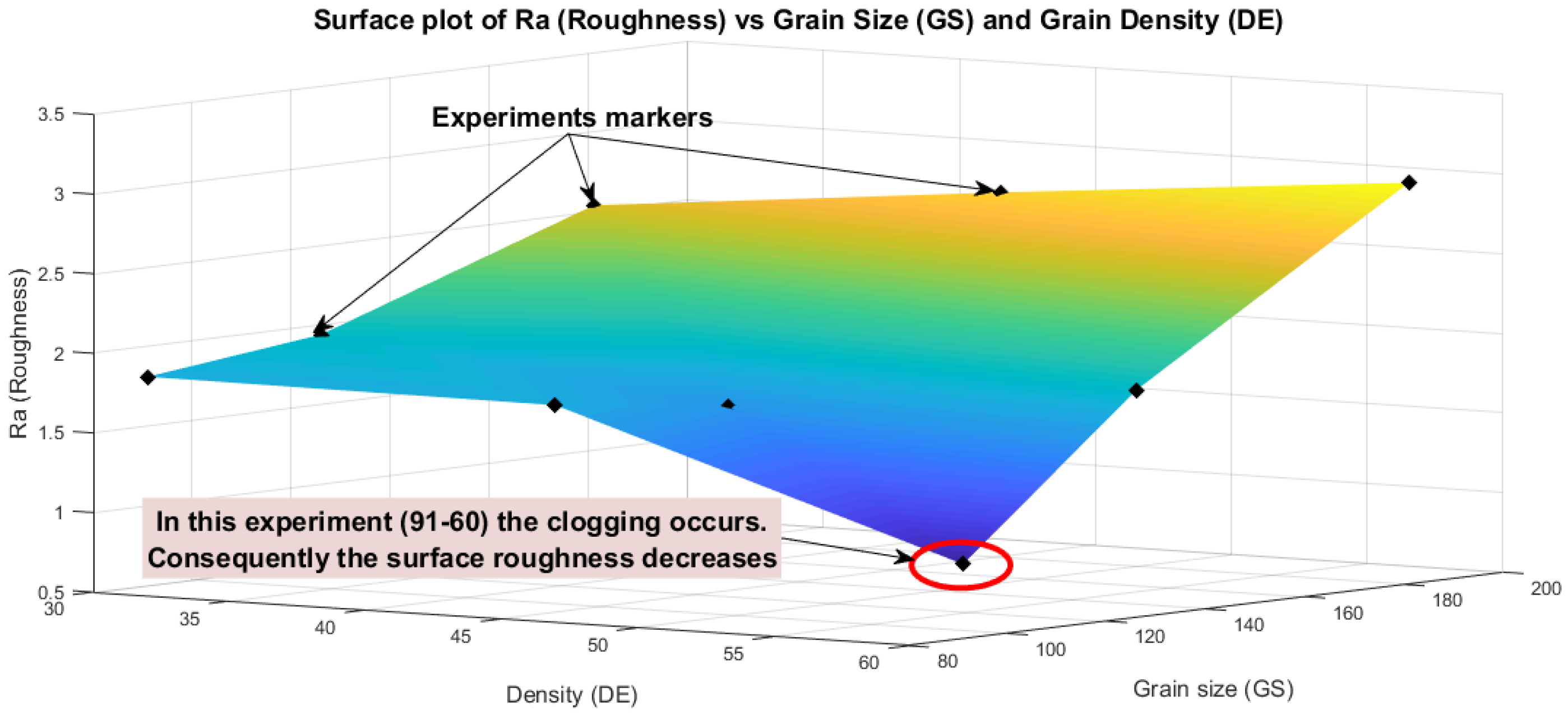
3.1. Roughness

Results of 2D roughness parameters Ra, Rz, Rk, Rpk, Rvk, Mr1, and Mr2, as well as 3D roughness parameters Sa and Sz are presented in

Table 2. Roughness results (average value of each experiment).

Experiment	Ra (μm)	Rz (μm)	Rk (μm)	Rpk (μm)	Rvk (μm)	Mr1 (%)	Mr2 (%)	Sa (μm)	Sz (μm)
1	3.02	18.02	9.17	4.79	3.67	10.78	89.50	3.27	27.82
2	2.79	16.57	8.73	4.02	3.65	11.28	89.37	2.77	23.48
3	2.54	15.45	7.85	4.09	2.71	12.35	91.20	2.61	22.89
4	1.93	12.64	5.89	2.87	2.47	10.71	88.17	2.00	17.70
5	1.66	10.90	5.06	2.45	2.38	9.59	88.70	1.76	15.37
6	1.94	12.44	5.85	2.81	2.77	10.72	89.46	1.93	18.35
7	0.97	6.58	2.86	1.27	1.32	9.89	87.94	0.97	10.93
8	1.80	11.66	5.43	2.80	2.31	11.78	89.15	1.76	15.71
9	1.81	11.67	5.61	2.62	2.00	11.40	90.05	1.91	15.74

for all experiments considered.

The highest Ra and Rz values correspond to high grain size of 181 and high abrasive density of 60 (experiment 1), while the lowest Ra and Rz values were obtained with low grain size of 91 and high density of 60 (experiment 7). The same trend was observed for 3D roughness parameters Sa and Sz. Lower Ra values are usual in honing processes after semi-finish and plateau honing operations [6]. As for the Abbott–Firestone parameters, obtained Rk, Rpk, Rvk, Mr1, and Mr2 values are higher than those recommended by the manufacturers [6,10]. It should be taken into account, however, that in the present paper only, the rough honing operation was performed, not the semi-finish or plateau honing operation. Especially low values for roughness parameters were reportedd for experiment 7, suggesting that peaks and valleys have been smoothed because of inappropriate cutting.

The regression models for the roughness parameters Ra, Rz, Rk, Rpk, Rvk, Sa, and Sz are presented in Equations (5)–(11), respectively, with their corresponding R²-adj value.

$$Ra=\mathbf{3.141}-\mathbf{0.00685}·\mathit{G}\mathit{S}-\mathbf{0.0661}·\mathit{D}\mathit{E}+\mathbf{0.00048}·\mathit{G}\mathit{S}·\mathit{D}\mathit{E}\left({\mathrm{R}}^2\text{-}\mathrm{adj}=85.38\%\right)$$

(5)

$$R{z}^{\mathbf{2}}=\mathbf{299}-\mathbf{0.915}·\mathit{G}\mathit{S}-\mathbf{8.56}·\mathit{D}\mathit{E}+\mathbf{0.0644}·\mathit{G}\mathit{S}·\mathit{D}\mathit{E}({\mathrm{R}}^2\text{-}\mathrm{adj}=82.76\%)$$

(6)

$$Rk=\mathbf{9.63}-\mathbf{0.0201}·\mathit{G}\mathit{S}-\mathbf{0.2068}·\mathit{D}\mathit{E}+\mathbf{0.001442}·\mathit{G}\mathit{S}·\mathit{D}\mathit{E}\left({\mathrm{R}}^2\text{-}\mathrm{adj}=85.16\%\right)$$

(7)

$$Rpk=\mathbf{4.58}-\mathbf{0.0091}·\mathit{G}\mathit{S}-\mathbf{0.1027}·\mathit{D}\mathit{E}+\mathbf{0.000725}·\mathit{G}\mathit{S}·\mathit{D}\mathit{E}\left({\mathrm{R}}^2\text{-}\mathrm{adj}=76.80\%\right)$$

(8)

$$Rvk=\mathbf{4.18}-\mathbf{0.0120}·\mathit{G}\mathit{S}-\mathbf{0.0831}·\mathit{D}\mathit{E}+\mathbf{0.000625}·\mathit{G}\mathit{S}·\mathit{D}\mathit{E}\left({\mathrm{R}}^2\text{-}\mathrm{adj}=66.63\%\right)$$

(9)

$$Sa=\mathbf{3.629}-\mathbf{0.01061}·\mathit{G}\mathit{S}-\mathbf{0.0782}·\mathit{D}\mathit{E}+\mathbf{0.000571}·\mathit{G}\mathit{S}·\mathit{D}\mathit{E}\left({\mathrm{R}}^2\text{-}\mathrm{adj}=86.69\%\right)$$

(10)

$$S{z}^{\mathbf{0.5}}=\mathbf{5.102}-\mathbf{0.00531}·\mathit{G}\mathit{S}-\mathbf{0.0586}·\mathit{D}\mathit{E}+\mathbf{0.000422}·\mathit{G}\mathit{S}·\mathit{D}\mathit{E}\left({\mathrm{R}}^2\text{-}\mathrm{adj}=80.20\%\right)$$

(11)

The amplitude parameters Ra, Rz, Sa, and Sz, as well as core roughness Rk have R²-adj values above 80%. However, reduced peak height Rpk and reduced valley depth Rvk show lower values of 76.80% and 66.63%, respectively.

As an example, Figure 2 depicts the surface plot for parameter Ra vs. grain size and density of abrasive grains.

As a general trend, roughness increases with grain size and density, as it had been found in previous experiments [38,39]. However, experiment 7, with grain size 91 and density 60, shows lower roughness than expected. This suggests that the tool crushes the material instead of cutting it. Figure 3a,b show magnified images of the abrasives’ surfaces after the honing operations, for experiments 2 and 7 respectively.

In Figure 3a, performed with grain size 181 and density 45 (experiment 2), sharp abrasive grains are observed. The bond surface shows several marks produced by the detached grains during the honing operation. This corresponds to a correct honing operation. On the contrary, Figure 3b shows a picture of the abrasive with grain size 91 and density of abrasive 60 (experiment 7). There, a more irregular surface is seen, in which abrasive grains are not clearly observed. Some grains are worn out, with smooth surfaces, and only few marks of detached grains are detected on the abrasive’s surface. This suggests that, due to the high density of abrasive, most grains crush the workpiece material rather than cutting it, and the chips fill the voids, leading to clogging.

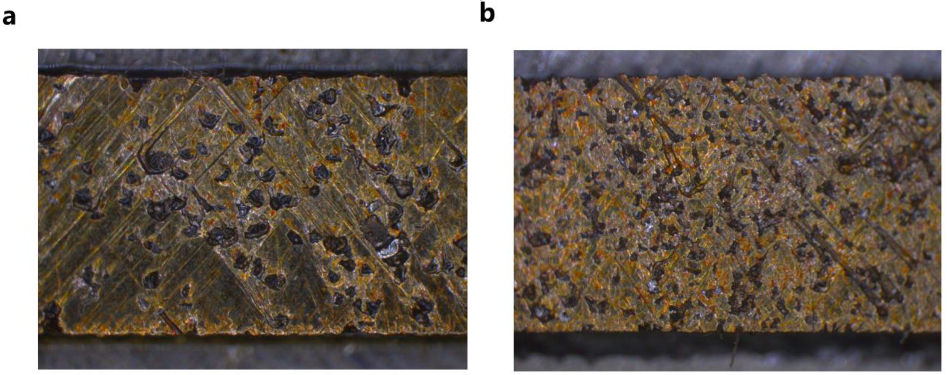
3.2. Material Removal Rate and Tool Wear

Results for material removal rate Qm (cm/min) and tool wear Qp (cm³/min) are presented in

Table 3. Material removal rate and tool wear results (average value of each experiment).

Experiment	Qm (cm/min)	Qp (cm3/min)
1	0.35	0.0008
2	0.26	0.0008
3	0.20	0.0006
4	0.19	0.0001
5	0.23	0.0002
6	0.15	0.0002
7	0.15	0.0002
8	0.24	0.0005
9	0.21	0.0006

for all experiments considered.

The highest Qm value of 0.35 cm/min corresponds to experiment 1, with high grain size of 181 and high abrasive density of 60, while the lowest Qm value of 0.15 cm/min was obtained in experiments 6 and 7, with medium grain size and low density, and low grain size and high density respectively. Obtained values are similar to those reported in the literature for CBN stones [12,13], although with high grain size and high density higher material removal rates of 0.35 cm/min are achieved.

The regression model for material removal rate Qm is presented in Equation (12), with its corresponding R²-adj value.

$${\mathit{Q}}_{\mathit{m}}=\mathbf{0.534}-\mathbf{0.002787}·\mathit{G}\mathit{S}-\mathbf{0.00925}·\mathit{D}\mathit{E}+\mathbf{0.000079}·\mathit{G}\mathit{S}·\mathit{D}\mathit{E}\left({\mathrm{R}}^2\text{-}\mathrm{adj}=63.98\%\right)$$

(12)

Figure 4 shows the effect of grain size and density on material removal rate Qm.

At high grain size, the higher the density, the higher the material removal rate, as expected. However, experiments performed at medium and low grain size combined with high density (experiments 4 and 7) lead to lower material removal rates and lower tool wear than those with lower density. This suggests that when density is too high for a certain grain size, abrasives do not cut properly because of clogging.

Low values were reported for tool wear for CBN stones, as expected, ranging between 0.0001 and 0.0008 cm³/min.

Cylindricity values before honing ranged between 13.75 μm and 38.06 μm, while cylindricity values after honing ranged between 19.75 μm and 52.76 μm. Similar cylindricity results were reported by Lei et al. [40].

3.3. Acoustic Signal Analysis

3.3.1. Initial Signal Treatment

As an example, the resampled signal of experiment 2 is depicted in Figure 5a. Then, autocorrelation was applied, in order to increase precision. In addition, the mean period of the honing cycle was extracted from the sound signal. It was found to be 0.492 s. Figure 5b represents the Fast Fourier Transform (FFT) of the signal of experiment 2. The harmonic components appear every 2.03 Hz, according to the honing cycle.

Figure 6a shows the auto crosscorrelation signal for experiment 2, and Figure 6b, its Fast Fourier transform FFT. There it is possible to confirm the honing cycle frequency of around 2.06 Hz.

3.3.2. Application of a Homomorphous Filter

The second step treatment of the signal involves cutting a certain length corresponding to several honing cycles. After this, the signal is decomposed into harmonic and non-harmonic parts, by means of a homomorphous filter. Figure 7 represents a signal containing three consecutive honing cycles. For frequencies between 130 and 18 Hz. Harmonic components are represented in red color, while non-harmonic components are highlighted in blue.

The harmonic part of the signal shows peaks that are separated from each other by 2.06 Hz.

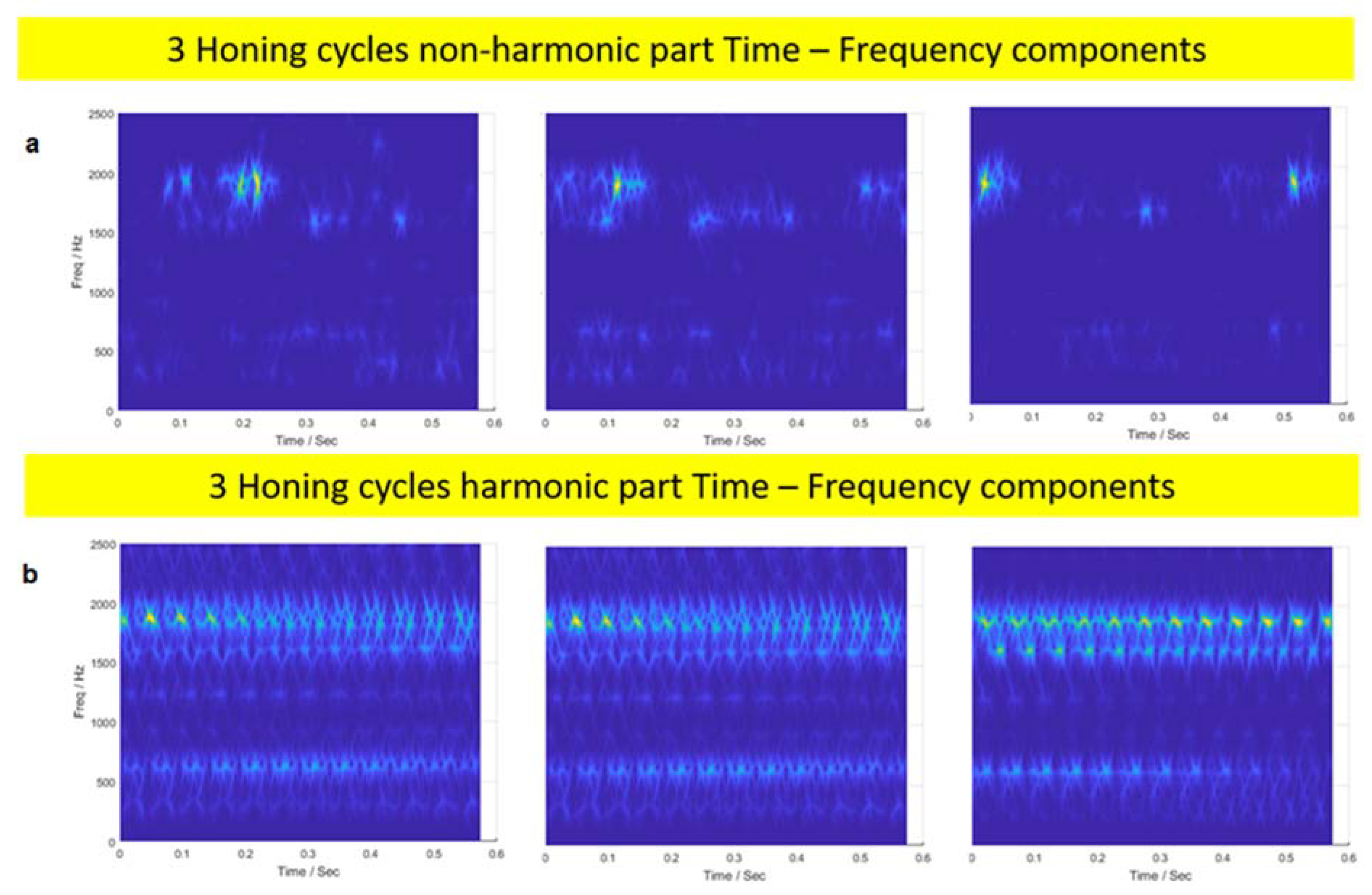
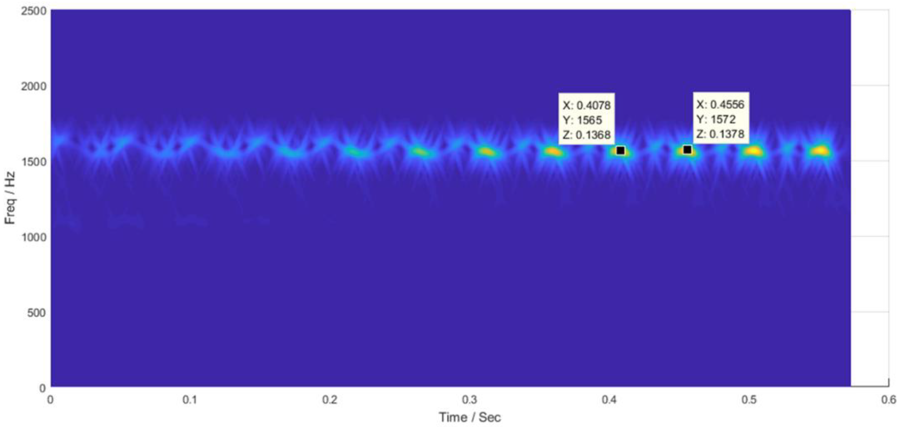
3.3.3. Application of the Chirplet Transform

The complete method described in Section 2 was applied to two different experiments in order to compare them. Experiment 2, with grain size 181 and density 45, corresponds to a correct honing process; experiment 7, with grain size 91 and density 60, shows lower roughness and material removal rate than expected, suggesting that clogging occurred

Regarding experiment 2, Figure 8 shows the time-frequency pictures from the chirplet application to both non-harmonic and harmonic parts of the signal of experiment 2. They correspond to three honing cycles of a correct honing process (every window corresponds to a honing cycle). Figure 8a contains the time-frequency peaks of the non-harmonic components, which probably correspond to the sound of the abrasive stone when the linear movement direction changes in every honing cycle. The highest peaks of highest frequency correspond to the outward stroke of the honing head. In Figure 8b (harmonic part), there is a stable pattern along the three honing cycles.

Figure 9a contains the values of frequency-time-amplitude at eight points of the second window of Figure 9b. The distance between successive marks corresponds to 20.4 Hz or 1224.5 min⁻¹. This value could be compatible with the rotation speed of the oil pump of the machine. Figure 9b contains the values of the harmonic frequencies. It is observed that the maximum amplitude varies throughout the cycle time. This could be attributed to a slight imperfection in the axis alignment between tool and cylinder, or to wear differences among the three abrasive stones, which can cause modulated harmonic perturbations.

As for experiment 7, where clogging occurs, the non-harmonic pattern (Figure 10a) is better defined than for experiment 2 (Figure 8a), with three important marks on each screen. The harmonic pattern (Figure 10b) also shows important differences with respect to that of experiment 7 (Figure 8b) because it is a non-stable pattern, showing frequencies that are contained within a narrower frequency band. The frequency for the rotational hydraulic pump is the same as for experiment 2 because the time between peaks is also 0.0478 s. Nevertheless, the frequency oscillates considerably with time when the machine is operating under clogging.

Figure 11 shows the pattern of the harmonic part of the third honing cycle considered. When the honing machining process works badly, the main frequencies change and the peak values (z values) increase considerably. The fact that the bands are time-varying is usually associated with problems in the part or in the process [31]. The harmonic pattern was not continuous, due to clogging, in contrast with a continuous harmonic pattern when the machine works correctly, as in experiment 2 (Figure 8b).

When the honing machine work under incorrect operating conditions, the main frequency changes from 1890–1836 Hz (Figure 8a) to a new, lower value of 1565–1572 Hz (Figure 11). In addition, the peaks’ amplitude increases from 0.005 to a new value of 0.450, approximately 90 times higher.

4. Discussion

The results of the present paper show that, as a general trend, roughness, material removal rate, and tool wear increase with grain size and density as expected [41,42,43]. However, when clogging occurs, unusually low values for the three a.m. properties are reported [44]. Roughness values obtained for grain size 91 and 46 lie within the 0.05–1.6 µm range, determined by Petropoulos et al. High grain size of 181 provided even higher Ra values up to 3.02 µm. Rk, Rpk, and Rvk values reported in the present paper for rough honing are higher than those found in the literature for finished honing [9,11]. This is because higher grain size is used in rough than in finish honing operations. Material removal rate values obtained here are similar to those reported in the literature for rough honing [12,13], except for high grain size and high density, with higher material removal rate.

Chirplet transform was applied to AE signals from the honing processes in order to detect the incorrect function of the process. The application of linear chirplet treatment to AE signals is, in a computational sense, easier and faster than other methods such as the Hilbert–Huang transform. Chirplet also offers interesting information about acoustic emission patterns from the honing processes, as can be seen in the time-frequency plots throughout the present paper. For example, a time-varying frequency pattern is usually associated with problems of a certain part or process [31].

The method presented here can be combined with Hilbert–Huang transform. Hilbert–Huang treatment requires two steps. First, the signal is decomposed by the Empirical Mode Decomposition (EMD), in order to obtain a family of signals from different frequency ranges, the Intrinsic Mode Functions (IMF’s). Second, the Hilbert transform is applied to each one in order to obtain the instantaneous frequency over time [44]. A hybrid treatment would consist of the calculation of EMD/IMF’s and chirplet application to each part of the signal.

The method can be extended in order to refine the analysis of harmonic components by reconstructing the harmonic part without some known fundamental components. The idea is to apply some selective filter process (paint, band, etc.) and to repeat the chirplet analysis. The objective is to magnify the rest of the harmonic components in the time-frequency plots, due to the fact that the most important components in the amplitude can be eclipsed by other components in the graphic representations. Thus, it can be stated that it is only possible to analyze the frequency zone of interest, eliminating the other components.

5. Conclusions

In the present paper, rough honing experiments were performed with different grain size and density of abrasive grains. Roughness, material removal rate, and tool wear were measured, and the AE signal was recorded. The main conclusions are as follows:

-

As a general trend, roughness, material removal rate, and tool wear increase with the grain size and density of the abrasive. However, when high density is combined with medium or low grain size, both roughness and material removal rate decrease, suggesting that clogging occurs.

-

AE signals vary for different cutting conditions. A new methodology, based on chirplet transform, is proposed here to analyze the acoustic emission signals. It consists of resampling the signals, and filtering them with a homomorphous filter to decompose the signal into harmonic and non-harmonic components. Afterwards, chirplet transform is applied to the decomposed signals.

-

Two different experiments were compared: one in which the honing operation was correct (grain size 181 and density 45), and another one with clogging (grain size 91 and density 60). When clogging starts, in both harmonic and non-harmonic chirplet diagrams, the patterns become non-stable. In the harmonic pattern, main frequencies decrease with clogging, and the amplitude of the pattern decreases. The results show that it is possible to successfully apply the chirplet analysis to detect the incorrect working of the honing operation.

The methodology presented here provides an easy and fast way to analyze whether a certain honing process is working properly. It can be used in the future to monitor the honing processes and to stop them if they are not working appropriately.

References

- Golloch, R.; Merker, G.P.; Kessen, U.; Brinkmann, S. Functional properties of microstructured cylinder liner surfaces for internal combustion engines. Tribotest J. 2005, 11, 307–324. [Google Scholar] [CrossRef]
- Deepak Lawrence, K.; Shanmugamani, R.; Ramamoorthy, B. Evaluation of image based Abbott–Firestone curve parameters using machine vision for the characterization of cylinder liner surface topography. Measurement 2014, 55, 318–334. [Google Scholar] [CrossRef]
- Lee, D.E.; Hwang, I.; Valente, C.M.O.; Oliveira, J.F.G.; Dornfeld, D.A. Precision manufacturing process monitoring with acoustic emission. In Condition Monitoring and Control for Intelligent Manufacturing; Wang, L., Gao, R.X., Eds.; Springer: London, UK, 2006; pp. 33–54. [Google Scholar]
- Ma, S.; Liu, Y.; Wang, Z.; Wang, Z.; Huang, R.; Xu, J.; Ma, S.; Liu, Y.; Wang, Z.; Wang, Z.; et al. The effect of honing angle and roughness height on the tribological performance of cunicr iron liner. Metals 2019, 9, 487. [Google Scholar] [CrossRef]
- Whitehouse, D.J. Handbook of Surface and Nanometrology; CRC Press: Boca Raton, FL, USA, 2003. [Google Scholar]
- Petropoulos, G.P.; Pandazaras, C.N.; Davim, J.P. Surface texture characterization and evaluation related to machining. In Surface Integrity in Machining; Springer London: London, UK, 2010; pp. 37–66. [Google Scholar]
- ISO 13565-2:1996. Geometrical Product Specifications (GPS)—Surface Texture: Profile Method; Surfaces Having Stratified Functional Properties—Part 2: Height Characterization Using the Linear Material Ratio Curve; ISO: Geneva, Switzerland, 1996; pp. 1–6.
- Feng, C.-X.; Wang, X.; Yu, Z. Neural networks modeling of honing surface roughness parameters defined by ISO 13565. J. Manuf. Syst. 2002, 21, 395–408. [Google Scholar] [CrossRef]
- Tribology and Dynamics of Engine and Powertrain: Fundamentals, Applications and Future Trends; Rahnejat, H., Ed.; Woodhead Publishing Limited: Cambridge, UK, 2010. [Google Scholar]
- Computational Methods for Optimizing Manufacturing Technology: Models and Techniques; Davim, J.P., Ed.; Engineering Science Reference: Hershey, PA, USA, 2012. [Google Scholar]
- El Mansori, M.; Goeldel, B.; Sabri, L. Performance impact of honing dynamics on surface finish of precoated cylinder bores. Surf. Coat. Technol. 2013, 215, 334–339. [Google Scholar] [CrossRef]
- Szabo, O. Examination of material removal process in honing: EBSCOhost. Acta Tech. Corviniensis-Bull. Eng. 2014, 7, 35–38. [Google Scholar]
- Vrac, D.; Sidjanin, L.; Balos, S. The effect of honing speed and grain size on surface roughness and material removal rate during honing. Acta Polytech. Hung. 2014, 11, 163–175. [Google Scholar]
- Liu, Q.; Chen, X.; Gindy, N. Fuzzy pattern recognition of AE signals for grinding burn. Int. J. Mach. Tools Manuf. 2005, 45, 811–818. [Google Scholar] [CrossRef]
- Lee, W.K.; Ratnam, M.M.; Ahmad, Z.A. Detection of chipping in ceramic cutting inserts from workpiece profile during turning using fast Fourier transform (FFT) and continuous wavelet transform (CWT). Precis. Eng. 2017. [Google Scholar] [CrossRef]
- Câmara, M.A.; Abrão, A.M.; Campos Rubio, J.C.; Godoy, G.C.D.; Cordeiro, B.S. Determination of the critical undeformed chip thickness in micromilling by means of the acoustic emission signal. Precis. Eng. 2016, 46, 377–382. [Google Scholar] [CrossRef]
- Bifano, T.G.; Yi, Y. Acoustic emission as an indicator of material-removal regime in glass micro-machining. Precis. Eng. 1992, 14, 219–228. [Google Scholar] [CrossRef]
- Webb, A.R. Statistical Pattern Recognition, 2nd ed.; Wiley: Chichester, UK, 2003. [Google Scholar]
- Belsak, A.; Flasker, J. Wavelet analysis for gear crack identification. Eng. Fail. Anal. 2009, 16, 1983–1990. [Google Scholar] [CrossRef]
- El-Thalji, I.; Jantunen, E. Fault analysis of the wear fault development in rolling bearings. Eng. Fail. Anal. 2015, 57, 470–482. [Google Scholar] [CrossRef]
- Sejdić, E.; Djurović, I.; Jiang, J. Time–frequency feature representation using energy concentration: An overview of recent advances. Digit. Signal Process. 2009, 19, 153–183. [Google Scholar] [CrossRef]
- Kanthababu, M.; Shunmugam, M.S.; Singaperumal, M. Identification of significant parameters and appropriate levels in honing of cylinder liners. Int. J. Mach. Mach. Mater. 2009, 5, 80–96. [Google Scholar] [CrossRef]
- Auger, F.; Flandrin, P. Improving the readability of time-frequency and time-scale representations by the reassignment method. IEEE Trans. Signal Process. 1995, 43, 1068–1089. [Google Scholar] [CrossRef]
- Yang, Y.; Dong, X.J.; Peng, Z.K.; Zhang, W.M.; Meng, G. Vibration signal analysis using parameterized time–frequency method for features extraction of varying-speed rotary machinery. J. Sound Vib. 2015, 335, 350–366. [Google Scholar] [CrossRef]
- Tse, P.W.; Wang, D. The design of a new sparsogram for fast bearing fault diagnosis: Part 1 of the two related manuscripts that have a joint title as “Two automatic vibration-based fault diagnostic methods using the novel sparsity measurement—Parts 1 and 2”. Mech. Syst. Signal Process. 2013, 40, 499–519. [Google Scholar] [CrossRef]
- Bianchi, D.; Mayrhofer, E.; Gröschl, M.; Betz, G.; Vernes, A. Wavelet packet transform for detection of single events in acoustic emission signals. Mech. Syst. Signal Process. 2015, 64–65, 441–451. [Google Scholar] [CrossRef]
- Hariharan, G.; Kannan, K. Review of wavelet methods for the solution of reaction–diffusion problems in science and engineering. Appl. Math. Model. 2014, 38, 799–813. [Google Scholar] [CrossRef]
- Cohen, L. Generalized phase-space distribution functions. J. Math. Phys. 1966, 7, 781–786. [Google Scholar] [CrossRef]
- Ashino, R.; Nagase, M.; Vailllancourt, R. Gabor, wavelet and chirplet transforms in the study of pseudodifferential operators (structure of solutions for partial differential equations). Surikaisekikenkyusho Kokyuroku 1998, 1036, 23–45. [Google Scholar]
- Luo, J.; Yu, D.; Liang, M. Application of multi-scale chirplet path pursuit and fractional Fourier transform for gear fault detection in speed up and speed-down processes. J. Sound Vib. 2012, 331, 4971–4986. [Google Scholar] [CrossRef]
- Peng, F.; Yu, D.; Luo, J. Sparse signal decomposition method based on multi-scale chirplet and its application to the fault diagnosis of gearboxes. Mech. Syst. Signal Process. 2011, 25, 549–557. [Google Scholar] [CrossRef]
- FEPA 61/97—FEPA Standard for Superabrasives Grain Sizes; Federation of European Producers of Abrasives: Darmstadt, Germany, 1997.
- Chatterjee, S.; Chatterjee, R.; Pal, K.; Pal, S.; Pal, S.K. Accurate Detection of Weld Defects Using Chirplet Transform. In International Conference on Computer and Automation Engineering, 4th (ICCAE 2012); ASME: New York, NY, USA, 2012; pp. 49–54. [Google Scholar]
- DIN 2391-Seamless Precision Steel Tubes, for Lines, Construction and Riveting, Cold Drawn, Unalloyed; Dimensions; DIN: Berlin, Germany, 1988.
- ISO 6104:2005—Superabrasive Products—Rotating Grinding Tools with Diamond or Cubic Boron Nitride—General Survey, Designation and Multilingual Nomenclature; ISO: Geneva, Switzerland, 2005.
- Mann, S.; Haykin, S. The chirplet transform: physical considerations. IEEE Trans. Signal Process. 1995, 43, 2745–2761. [Google Scholar] [CrossRef]
- Li, X. A brief review: Acoustic emission method for tool wear monitoring during turning. Int. J. Mach. Tools Manuf. 2002, 42, 157–165. [Google Scholar] [CrossRef]
- Buj-Corral, I.; Vivancos-Calvet, J.; Rodero-De-Lamo, L.; Marco-Almagro, L. Comparison between mathematical models for roughness obtained in test machine and in industrial machine in semifinish honing processes. Procedia Eng. 2015, 132, 545–552. [Google Scholar] [CrossRef][Green Version]
- Sivatte-Adroer, M.; Llanas-Parra, X.; Buj-Corral, I.; Vivancos-Calvet, J. Indirect model for roughness in rough honing processes based on artificial neural networks. Precis. Eng. 2016, 43, 505–513. [Google Scholar] [CrossRef]
- Lei, X.; Song, H.; Xue, Y.; Li, J.; Zhou, J.; Duan, M. Method for cylindricity error evaluation using Geometry Optimization Searching Algorithm. Measurement 2011, 44, 1556–1563. [Google Scholar] [CrossRef]
- Bell, S.B.; Maden, H.; Needham, G. The influence of grit size and stone pressure on honing. Precis. Eng. 1981, 3, 47. [Google Scholar] [CrossRef]
- Buj-Corral, I.; Vivancos-Calvet, J.; Coba-Salcedo, M. Modelling of surface finish and material removal rate in rough honing. Precis. Eng. 2014, 38, 100–108. [Google Scholar] [CrossRef]
- Buj-Corral, I.; Rodero-De-Lamo, L.; Marco-Almagro, L. Use of results from honing test machines to determine roughness in industrial honing machines. J. Manuf. Process. 2017, 28, 60–69. [Google Scholar] [CrossRef]
- Buj-Corral, I.; Álvarez-Flórez, J.; Domínguez-Fernández, A. Acoustic emission analysis for the detection of appropriate cutting operations in honing processes. Mech. Syst. Signal Process. 2018, 99, 873–885. [Google Scholar] [CrossRef]