Abstract
In this study, a water-model experiment and numerical simulation were carried out in a pilot ISASMELT furnace to study the factors affecting mixing time. The experimental results were compared to the simulation results to test the accuracy of the latter. To study the internal factors that affect the mixing time, the turbulent viscosity and flow field were calculated using simulation. In addition, following previous research, external factors that influence the mixing time including the depth of the submerged lance, lance diameter, gas flow rate, and the presence of a swirler were studied to investigate their effect on the flow regime. The results indicated that the mixing time is controlled by the turbulent viscosity and velocity vector. In addition, it was found that the lance diameter should not exceed 3.55 cm to maintain sufficient energy for stirring the bath. Finally, the optimal gas flow rate that offers the best mixing efficiency was found to be 50 Nm3/h.
1. Introduction
An ISASMELT furnace is an upright cylindrical furnace equipped with a top submerged lance (TSL). It is used to obtain matte from copper concentrate [1]. This furnace can achieve high intensity, autogenous smelting with considerable throughput. In an ISASMELT furnace, the heat generated through the chemical reaction maintains the temperature and additional fuel is sometimes added for temperature control.
In smelting, copper concentrate is fed from the top of the ISASMELT furnace, where the copper sulfide particles are subjected to heat that causes their primary decomposition. The high temperature and strong oxidizing atmosphere cause copper to further react and form matte (Cu2S-FeS), slag (2FeO·SiO2), and other substances. The rate of the reactions as well as mass and heat transfers are increased through vigorous agitation aided by oxygen-enriched air blown from the top of the furnace throughout the reaction process. Therefore, controlling the air blowing process can improve the furnace smelting conditions. Other operational conditions that affect the efficiency of the plant should also be studied and optimized. However, directly performing this type of study in an actual, experimental, or a pilot plant is impractical and uneconomical. The development of computational fluid dynamics (CFD) has allowed the study of many physical phenomena involving fluid flow and heat conduction through numerical simulation. Therefore, it has become an indispensable tool for the design and optimization of sophisticated chemical reactors [2,3,4], which are frequently used in the metallurgical industry. For example, CFD is used to study the decarburization process in argon oxygen decarburization converters and the multiphase flow phenomenon in Peirce-Smith converters. Also, in some research, user-defined function (UDF) technology is used to consider chemical reactions and slag splash, etc.
Forty years ago, Nakanishi et al. [5]. were the first to introduce mixing time as a parameter for investigating the mass transfer efficiency in steel refinery ladles or converters. This method is still widely used in the metallurgical industry. In addition, several studies have investigated the relationship between mixing time and several process parameters. The research conducted by Lang et al. [6] and Zhao et al. [7,8] proved that the mixing time is affected by the tracer addition and measuring positions, vessel geometry, gas flow rate, and liquid viscosity. Conversely, improving the mixing efficiency can significantly improve the smelting intensity. Also, different furnaces require different mixing times.
Since the first work reported by Schwarz and Koh [9], several researchers have focused on the topic of numerical simulation of the mixing process in a TSL furnace [10,11,12,13]. Huda et al. [14] compared the experimental and simulation results of velocity fields and turbulence generation in TSL smelting, and studied the effect of swirling and non-swirling flows inside the bath of an isothermal air-water system. However, these results are not sufficient to explain the mixing process caused by velocity fields, which is better explained through transport equations. Zhu et al. [15] performed a numerical study on a three-dimensional turbulent fluid flow, investigating the mixing characteristics in gas-stirred ladles while taking into consideration the nozzle position, the location from which the tracer is introduced, and gas flow rate.
Lee et al. [16] developed a numerical simulation program that predicts the fluid flow in the gas-stirred ladle with a submerged lance and pointed out that at a relatively low gas flow rate, the mixing time is affected by the position from which the tracer is introduced while at a very large gas flow rate, it hardly affects the mixing time. Wang et al. [17] established a mathematical model that studies two-phase flow and heat-transfer in ISASMELT furnaces and investigates the effect of gas flow rate and lance submergence depth on the temperature distribution to optimize the operation in the ISASMELT furnace. Ramirez-Argaez [18] simulated a two-phase gas-stirred ladle to study the effect of gas flow rate, injector position, number of injectors, and geometry of the ladle on the mixing efficiency. This study proved that increasing the gas flow rate enhances the mixing efficiency in the ladle, which is contradictory to the results of Lee et al.’s study [16]. This can be attributed to the difference in the furnace type, since Lee et al.’s study used TSL technology, while Ramirez-Argaez’s study used bottom injection. However, more data is needed to define the parameters affecting the mixing time.
Wang et al. [19] studied the flow characteristics in the system of gas injection into liquid through a top-submerged lance. The volume of fluid (VOF) multiphase model coupled with three turbulence models, renormalization-group (RNG), Reynolds stress model (RSM) and large eddy simulation (LES), have been considered and particle image velocimetry (PIV) experimental data was measured to verify the simulated results. The results showed that the 3D VOF-LES model had better agreement with the experimental data with regard to capturing the vortex and describing the bubble behavior and surface fluctuation. Adib et al. [20] studied the oscillatory phenomenon of the liquid surface in a non-submerged high-speed gas injection system using a VOF multiphase model coupled with a k−ω SST turbulence model. A cold-water model was implemented to verify the interface deformation and cavity depth.
In this study, the mixing behavior in a TSL gas-liquid system was investigated. The effects of gas flow rate, the diameter of the lance, and the presence of swirling on the mixing time were determined by numerical simulations and cold-water experiments.
2. Experiment
2.1. Water-Model Experiment
Based on the principle of geometric similarity, a cold-water model and a mathematical model were established for a prototype of an ISASMELT furnace (ISASMELT™, Brisbane, Australia) installed in the Chambishi Copper Smelter using a scale of 1:10 [8]. The water model was used to validate the accuracy of the numerical simulation. Water and air were selected to simulate the liquid phase in a molten pool and oxygen-enriched air blowing from the top, respectively. In the experiment, saturated NaCl solution was added to water to simulate the process of species diffusion and homogenization characterized by the mixing time. Typically, the mixing time is calculated from the moment of saturated NaCl solution addition to the moment when the conductivity of the mixture reaches 95% to 105% of the final (equilibrium) value [21,22]. There are four commonly used methods to measure the mixing time: conductivity, pH, electrical resistance tomography, and photoelectric cell methods. The last method is carried out by measuring the transmittance of light in a small volume of liquid to obtain the mixing time [23]. In this study, the conductivity method was adopted.
The gas-injected flow is primarily controlled by gravity and inertial forces, and thus, the modified Froude numbers (Fr′) of the experimental model and the industrial prototype must have the same value, which can be used as a reference value for industrial ISASMELT furnaces. Gas flow rate was determined basing on the dynamic similarity criterion. the Fr′ between the experimental model and real furnace can be expressed as [7]:
where ρg and ρl are the gas and liquid phases densities, respectively; g is the acceleration due to gravity; h is the height of the liquid level; and u is the gas inlet velocity. The velocity u can be calculated using the following formula:
where Q is the total gas volume under standard conditions, A is the area of lance outlet and d is the lance inlet diameter. The gas volume in the water-model experiment can be obtained using Equations (1) and (2). The Q used in the experimental model can be calculated by Equation (3). Table 1 shows a comparison between the experimental parameters in the industrial ISASMELT furnace and the water-model.

Table 1.
Parameters of water-model and ISASMELT furnace.
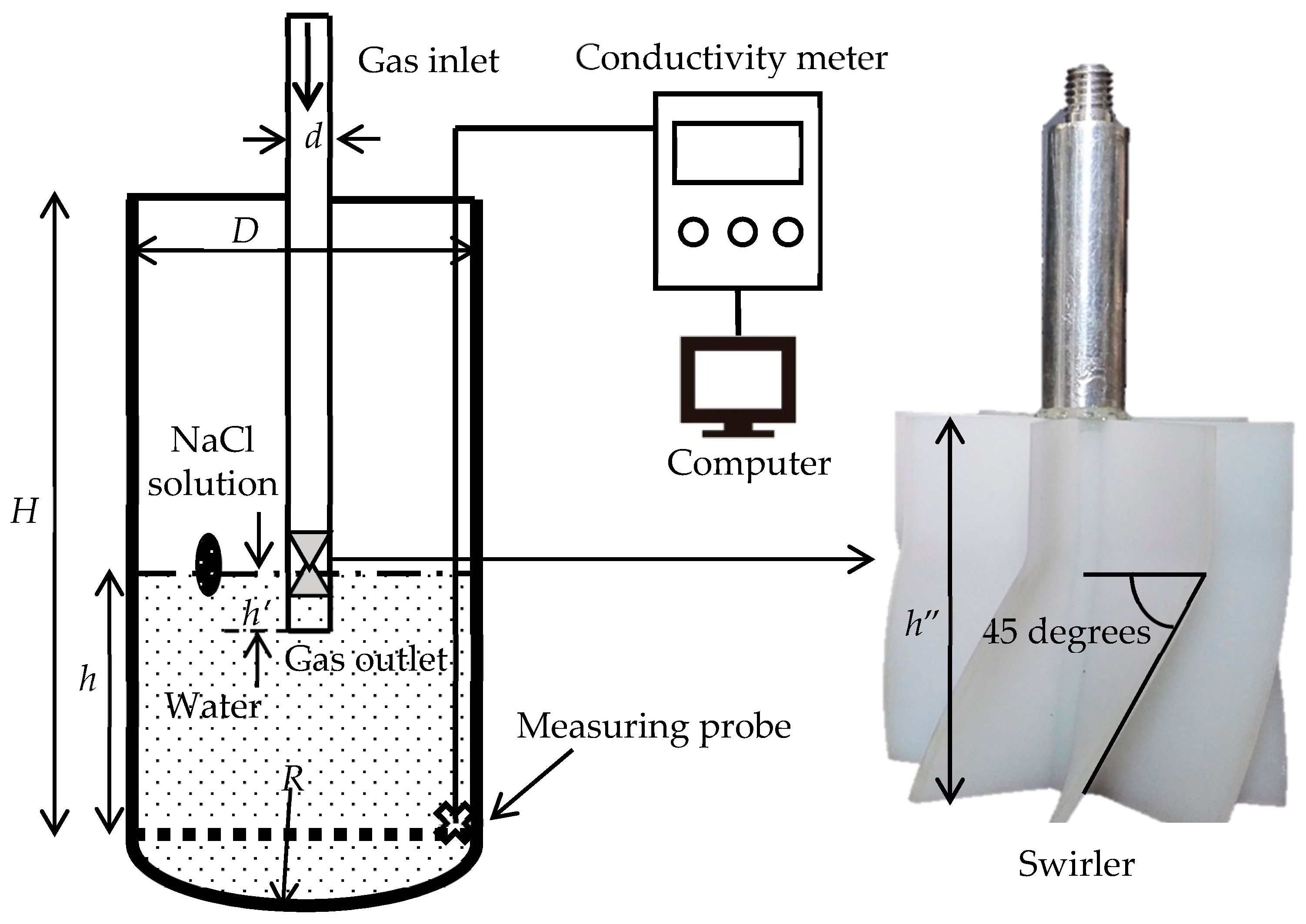
In the water-model experiment, the top-blown gas was injected in the bath through a submerged lance causing the water to fluctuate and splash. After the volume of the flow in the bath has stabilized and ceased to expand, 3 mL of saturated NaCl solution was added to the bath. Simultaneously, the change in the conductivity of the aqueous solution was monitored using a conductivity meter during a five-minute period. Geng et al. [24] proved that the mixing time is related to the position of the tracer addition in the vessel. In this experiment, Figure 1 illustrates that the location of the tracer addition is consistent with the industrial feeding location. The experiment was repeated five times under the same conditions and the average value of the mixing times was used in the calculations. In addition, the measurements were collected from different monitoring locations and the mean value was used.
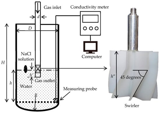
Figure 1.
Schematic diagram of the water model for measuring mixing time.
2.2. Governing Equations
A transient Eulerian two-phase model was developed using the volume of fluid model (VOF) method. In addition, the realizable k-ε turbulence model [25] was applied using the ANSYS Fluent (Version 14.0, ANSYS, Inc., Canonsburg, PA, USA) Fluent commercial software to simulate the complex fluid flow with both high and low Reynolds numbers. The realizable k-ε model, which has higher reliability for rotational flow, was adopted instead of the standard k-ε because the inlet gas flows in a spiral pattern after it passes through the swirl plate. The boundary conditions set in the water model were adopted here. The species transport equation and the flow field were used to study the diffusion process of the saturated NaCl solution in water after the formation of a steady flow field.
According to the VOF model, the continuity and momentum equations can be written as follows:
(1) Continuity equation
where q stands for phase q, αq is the volume fraction of phase q, is the velocity vector of the fluid and ρq is the density of phase q. The continuity equations are similar for all phases and the sum of αq must be equal to one.
(2) Momentum equation
where p is the static pressure, μ is the molecular viscosity, and is the gravitational body force. ρ and μ in each cell can be calculated using the following equations:
where n is the total number of phases.
(3) Turbulent flow equation
The realizable k-ε model is also a two-equation turbulence model, in which k and ε transport equations are solved. The transport equations used to calculate turbulence kinetic energy and turbulence energy dissipation can be expressed as
and
where
where S is the modulus of the mean rate-of-strain tensor; C2 is a constant; σk and σε are the turbulent Prandtl numbers for k and ε, respectively; and Gk is the generation of turbulence kinetic energy due to the mean velocity gradients:
where μt is the turbulent viscosity and can be calculated as:
where Cμ is a function of the mean strain, rotation rates, angular velocity of the system rotation, and turbulence fields.
(4) Species equation
ANSYS Fluent can model the mixing and transport of chemical species by solving conservation equations describing convection, diffusion, and the reaction sources for each component. Therefore, in the simulation conducted using Fluent, it was assumed that the tracer has similar properties as the liquid in the ISASMELT furnace and the tracer is located at the same position at which the saturated NaCl solution is added to water. The species transport equation was based on the average flow field, and several monitors with different positions were studied for a complete understanding of the tracer mixing process. It should be noted that the effect of splash in the species transport process was ignored; however, the splash phenomenon could possibly have some impact on the results of the experiment. The species transport equation is given as follows:
where , is the local mass fraction of species i, is the coefficient of mass diffusion of species i in the mixture ( is assumed to be 10−8 m2·s−1 [12]), and is the turbulent Schmidt number (the default value of is 0.7). Molecular diffusion is taken into account in the simulation, although it plays a small role in turbulence diffusion. A significant difference between the realizable k-ε and standard k-ε models is their treatment of turbulent viscosity, in which is equal to 0.09 in the standard k-ε model and is a variable in the realizable k-ε model.
The species transport equation demonstrates that turbulent viscosity plays an important role in turbulent species transport. Thus, the statistical averages of k, ε, and turbulent viscosity were calculated.
2.3. Numerical Methods and Boundary Conditions
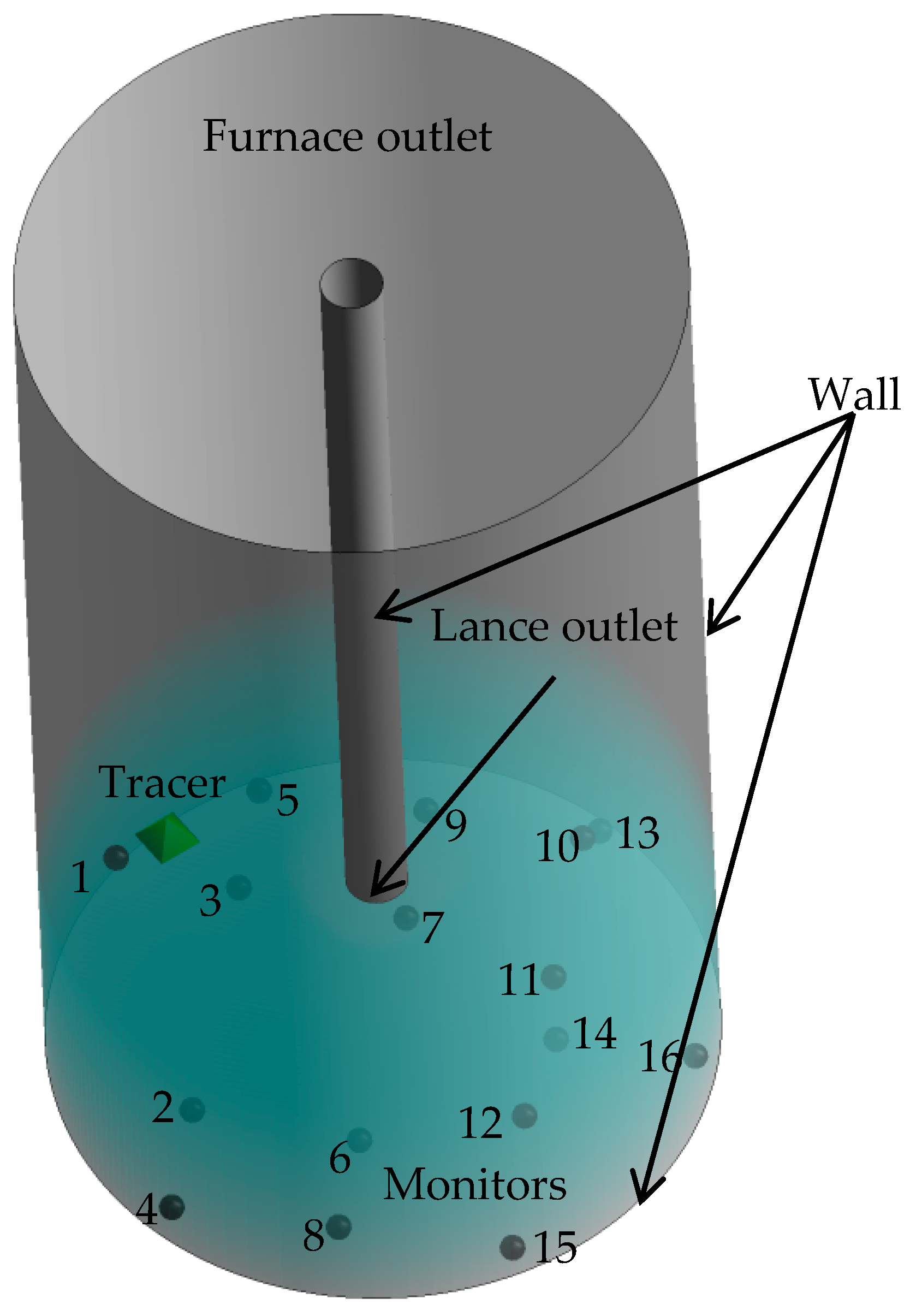
In this study, a velocity inlet boundary condition based on the lance geometry was used along with a pressure outlet boundary condition. In the gas-liquid two-phase system; the phase of both the inlet and outlet was found to be 100% gas phase. The furnace and the lance wall were set as a “no slip” wall condition. Figure 2 illustrates the boundary conditions and monitoring points.

Figure 2.
Boundary conditions and location of monitors.
The Navier–Stokes equations were solved using a finite volume method via a pressure-velocity coupled pressure-implicit with splitting of operator algorithm. The iterative residual of all primary variables was set at 10−4, and second order upwind spatial discretization was used for the momentum, k and ε. The pressure implicit scheme with splitting of operator pressure-velocity coupling (PISO) scheme was combined with a segregated solver to obtain accurate results and improve the efficiency of the calculations.
2.4. Mesh Model
Three-dimensional mixed meshes of tetrahedron and hexahedron were generated for the lance model, and meshes of hexahedron were generated for the furnace model. The total mesh numbers for the lance and furnace models were 100,000 and 600,000, respectively, which ensured the mesh-independent of simulated results.
3. Results and Discussions
3.1. Gas-Liquid Distribution during Injection Process
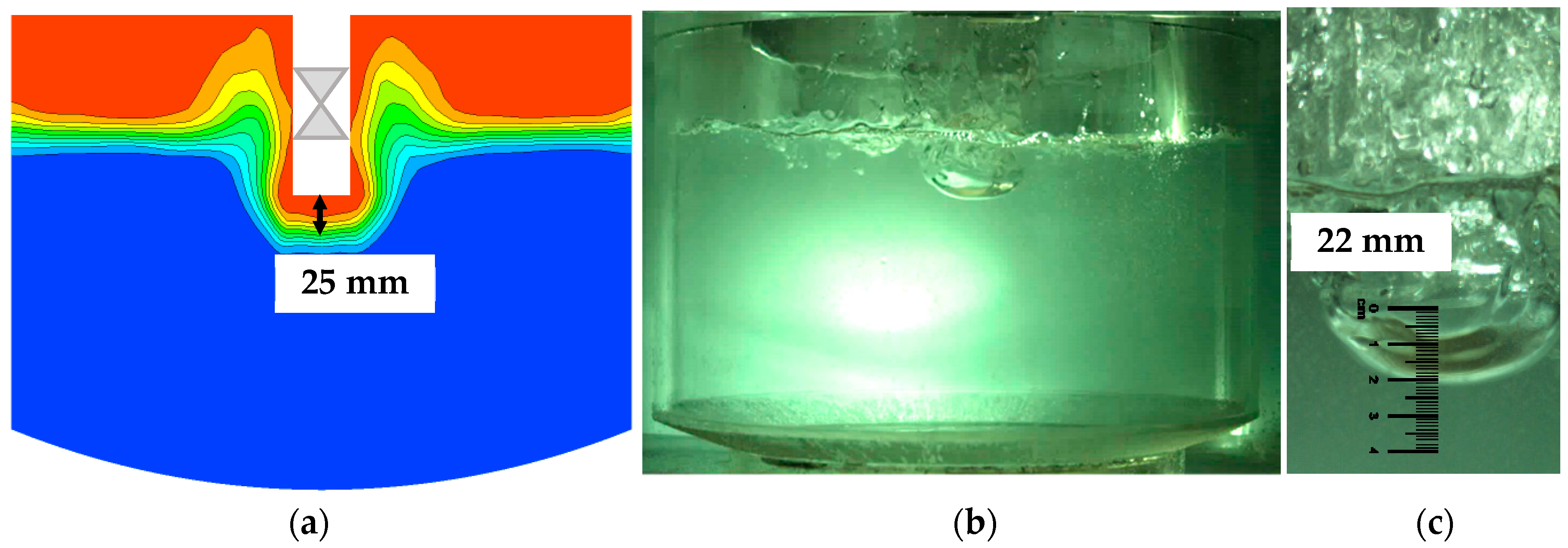
A high-speed camera (Fastec Imaging, San Diego, CA, USA) was used to record the gas injection process in the cold-water experiments, and the simulation was calculated under the same conditions of Q = 45 Nm3/h, d = 0.035 m, h = 0.04 m and swirler lance. The bubble was injected into the water liquid periodically in both the simulation and experiments. The gas penetration depth in the simulation was determined based on a mean statistical flow field. The gas penetration depth was defined as the height between the lance outlet and the iso-surface with a gas volume fraction of 0.5. In the experiment the gas penetration depth was measured from the high-speed picture when a stable bubble formed. The results of the bubble shape and gas penetrated depth showed good agreement between the simulated and experimental results as shown in Figure 3.

Figure 3.
Comparison of gas-liquid distribution between experimental the simulated results. (a) Simulated result, (b) experimental result and (c) measuring of gas penetrated depth.
3.2. Effect of Lance Submergence Depth and Swirler on Mixing Time
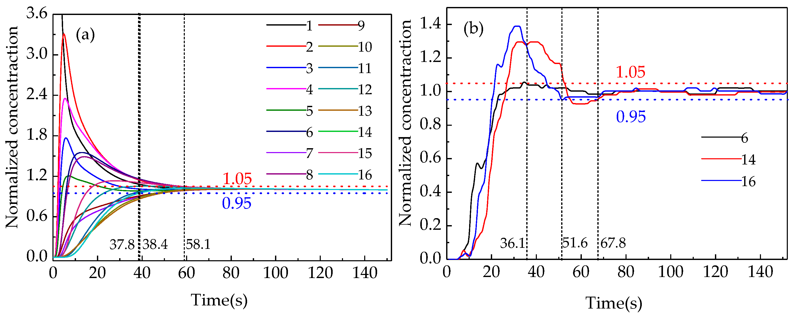
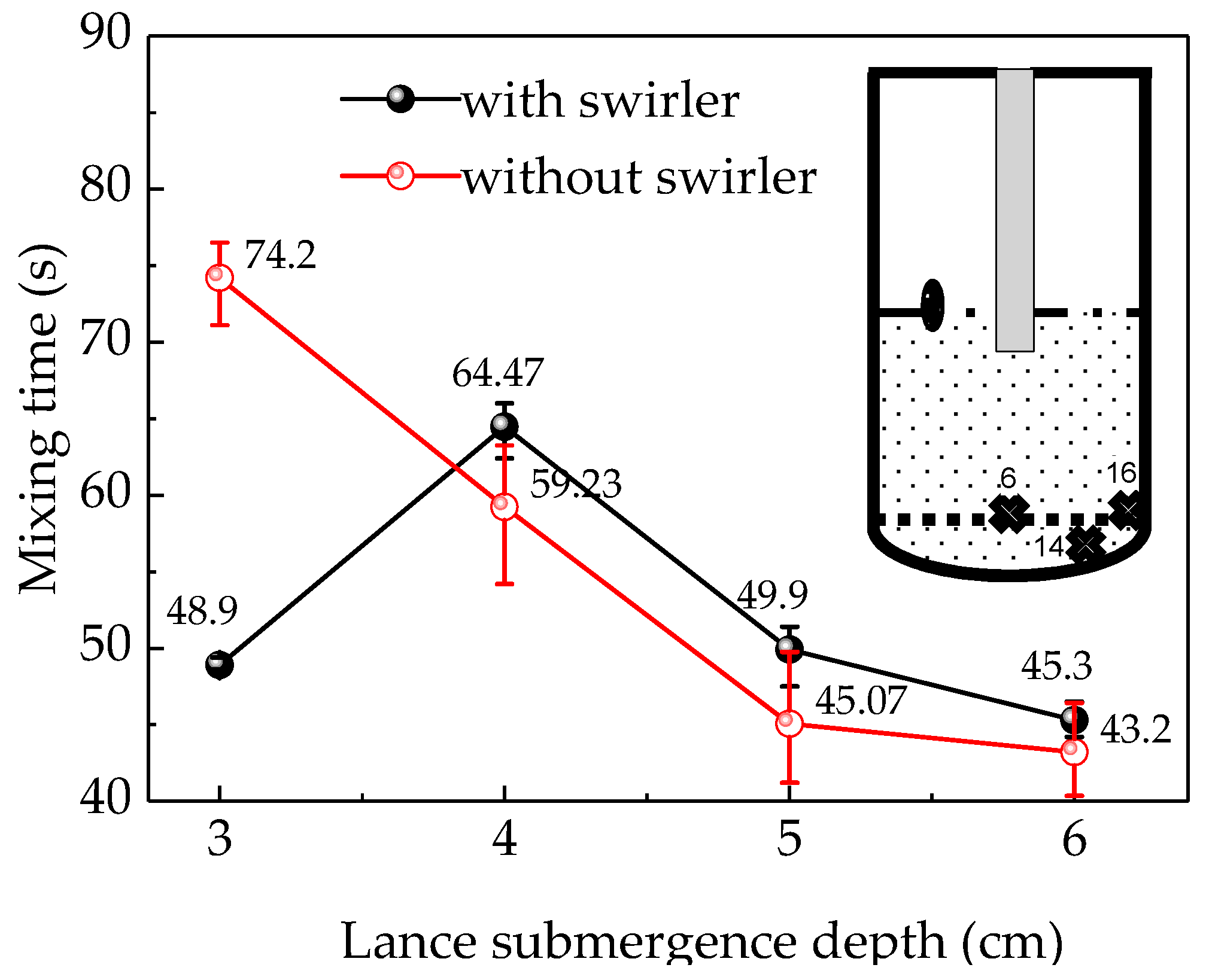
In order to verify the accuracy of the numerical simulation, the mixing time was measured when a lance with and without a swirler was used at lance submergence depths from 3 to 5 cm in the water-model platform. Figure 4 shows the curves of the tracer concentration over time for the 16 monitors illustrated in Figure 2 in the simulations and the selected three corresponding points in the experiments. The mixing time could be identified when the fluctuation of the tracer concentration was less than ±5% and the mean value of the mixing times were calculated with at least two-way simulation repetition experiments for each condition of gas flow rate, lance diameter and lance depth. Figure 4 indicates that the mixing times at different monitors under the same conditions were different. The points near the side wall and at the bottom have longer mixing time than other points and the uniform mixing time is decided by the point with the longest mixing time. Three points, namely point 16 (near the furnace wall), point 14 (on the bottom between the furnace center and the side wall) and point 6 (in the furnace center and near the bottom) were selected to compare the mixing efficiency under different conditions of submergence depths, lance diameters and gas flow rates.
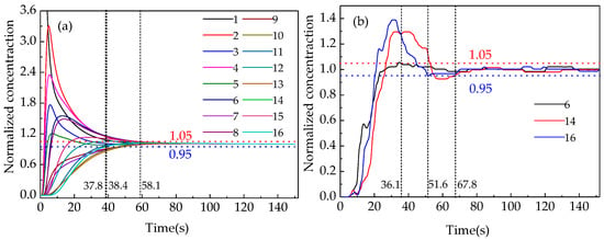
Figure 4.
Variation in the tracer concentration at different monitoring points. (a)Simulated curves and (b) experimental curves.
Figure 5 shows the mean mixing time of the three monitors (points 6, 14, 16) where it is relatively difficult to obtain uniform mixing in the water-model experiment. There was no significant difference between the mixing times at different monitors, which were within 3 s with a swirler and within 5 s without a swirler. This may be attributed to using multiple trials to determine the mean value of the mixing time, which covers the error due to the turbulence pulsation or to the inaccuracy of the conductivity meter in the detection of the change in the low tracer concentration. Therefore, the average value of multiple experiments was considered instead of a single value to reduce the error because the reading at the same point differs from one trial to another. To further reduce the experimental error, the average value of the mixing times at the three monitors was used as the final result.
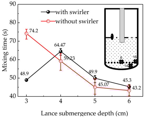
Figure 5.
The relationship between mixing time and lance submergence depth.
According to previous research, the mixing time estimated using the numerical simulation is slightly higher than that determined experimentally. This longer mixing time can be attributed to the fact that the mixing criteria is checked at every cell in the computation domain, while the mixing time determined experimentally is obtained by measuring the solute concentration in a single point in the tank [26].
The splash produced by the top-blown gas, which may contain NaCl solution, slowly flows along the wall of the furnace to the liquid phase resulting in the delay of the mixing process in the experiment. In addition, all the mixing times in the experiment and numerical simulation were obtained at a limited number of monitors instead of measuring them at every location. Furthermore, the simulation is based on using the average flow field in the species transport equation, which means the effect of splash is neglected. Based on all these reasons, the results of the simulation were less than those of the experiment.
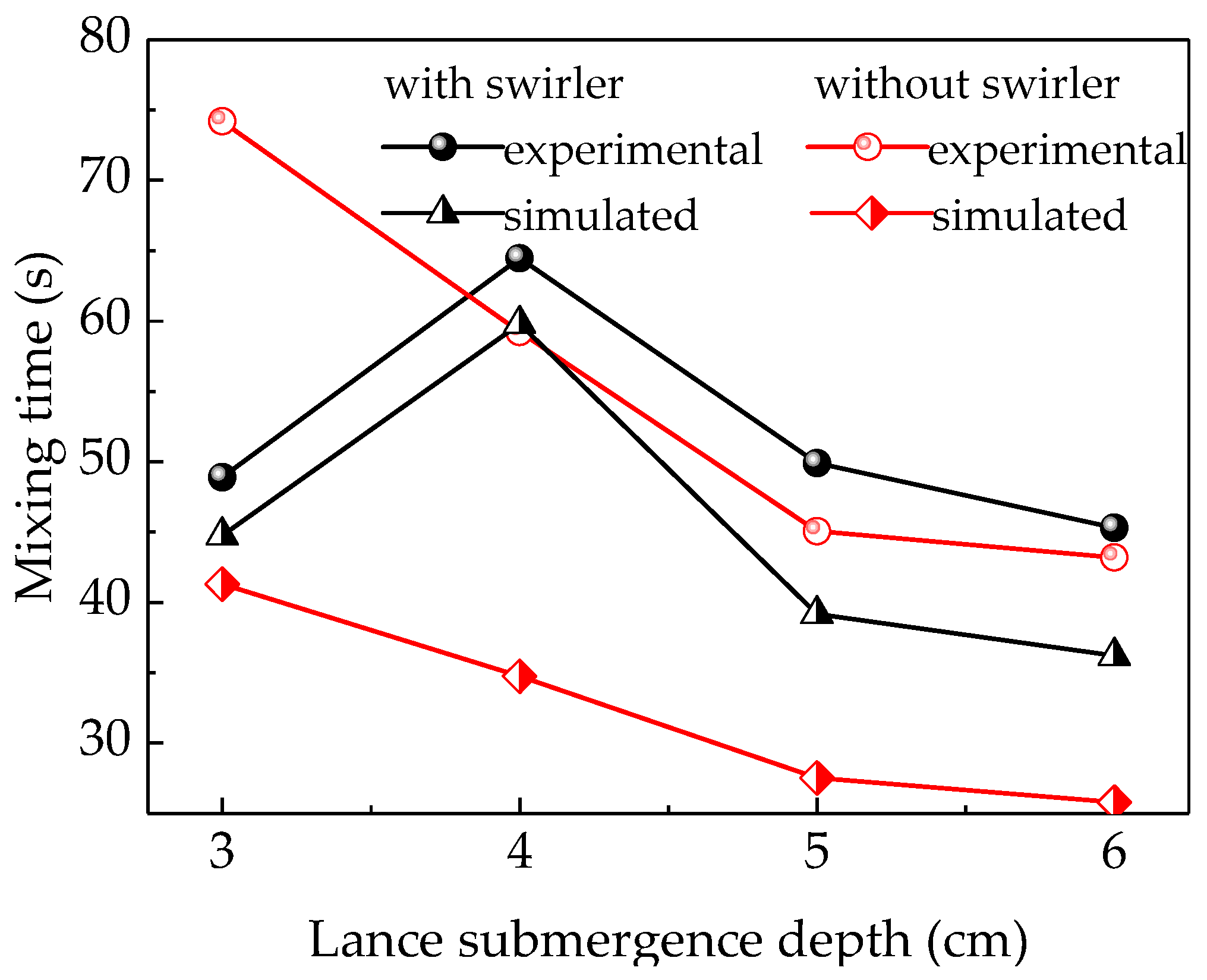
Figure 6 indicates that the simulation and experimental results followed similar patterns with regard to the lance submergence depth. In addition, the difference between the simulation and experiment results was smaller in the swirler case compared to the no-swirler case. The experimental data indicates that the mixing time was first increased to 65.73 s and then decreased to 49.63 s when the lance submergence depth equipped with a swirler changed from 3 to 5 cm, respectively. On the other hand, the mixing time without a swirler initially decreased from 71.7 s to 54.2 s and then to 40.2 s when the lance submergence depth increased. With a further increase in lance submergence depth, the mixing time decreased slightly, which may be due to the strong splashing on the liquid surface. The experimental mixing time without a swirler is longer than the simulated results, and the difference between the experimental and simulated results is larger than with a swirler. Firstly, the difference between the experimental and simulated results without a swirler may be caused by the serious surface slopping and splashing. [27] The tracer added into the liquid and its mixing may be disturbed by the splashing. When the tracer moves out of the liquid with the splashing, the mixing time would be extended. Especially, when the tracer moves to the vessel side wall, it may cost much time for tracer to flow down to the liquid. In the simulations, the splashing influence was ignored. So, the difference between the experimental and simulated results for the “no swirler” option is huge. When using the lance with a swirler, the splashing was reduced due to the rotated movement of the liquid. So, the difference between the experimental and simulated results is smaller. Secondly, the convective mixing for swirl flow is stronger than that of non-swirl flow. The rotating swirl flow could create a centrifugal force field which has a favorable convection effect in the molten bath. [14,28] The mixing behavior of tracer could be improved by a fully developed flow field. The rotational flow was generated when using a swirler, which may promote the convection diffusion of tracer species. When using the no-swirler lance, the liquid flow was only stirred by the periodic up-and-down motion and spread slowly, and the tracer moved with the liquid flow stirred by the periodic up-and-down moving bubbles. So, the liquid flow field spread slowly from the furnace center to the outside without the swirler. In addition, the rotation flow, especially vortex flow, could weaken the splashing on the liquid surface. Thirdly, the swirler was conducive to the formation of fine bubbles, which have better penetrated volume efficiency than large ones when increasing the tangential velocity and injected air flow rate [29].
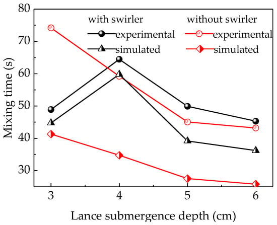
Figure 6.
Comparison between the mixing times estimated experimentally and using simulations.
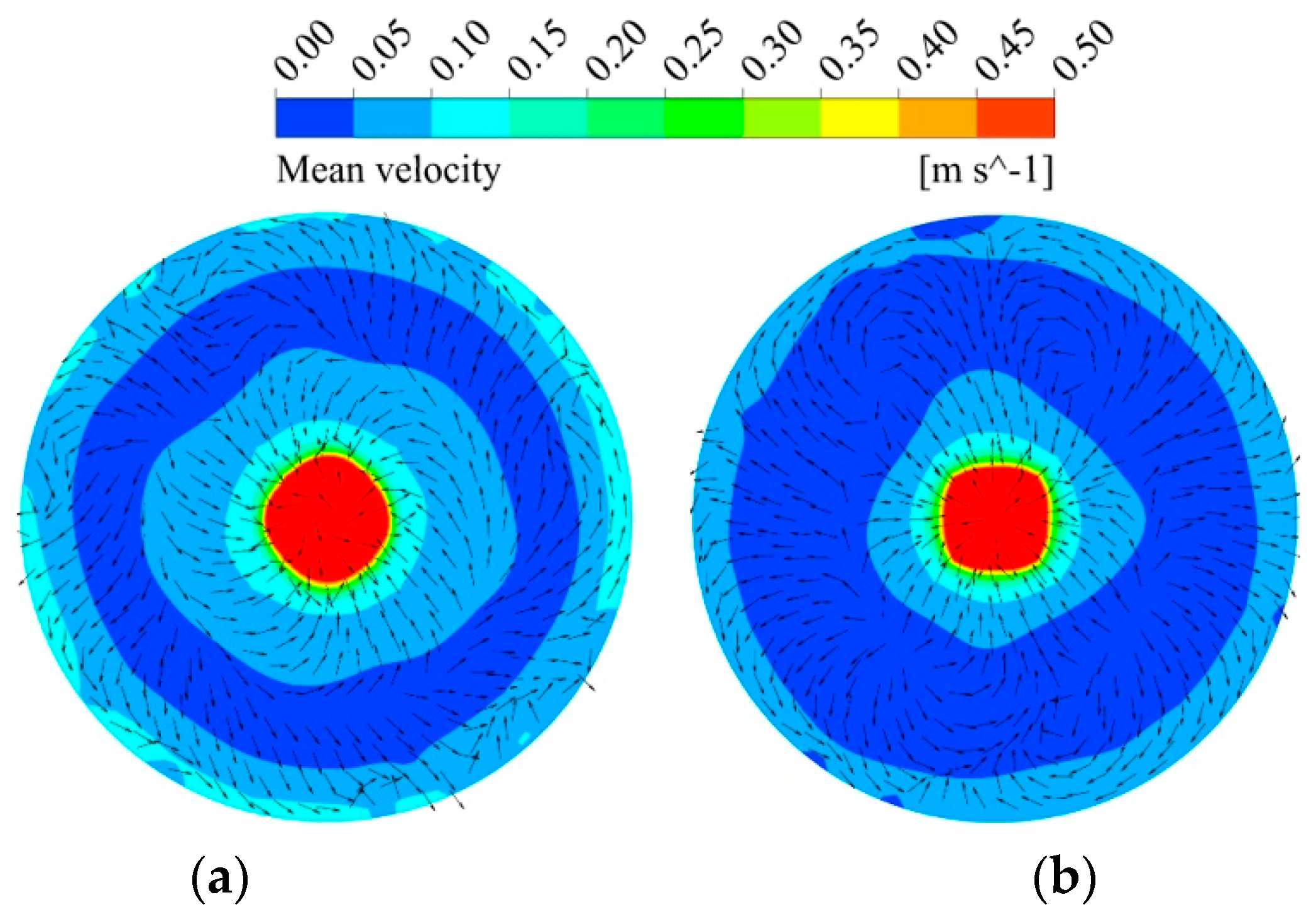
Figure 7 shows the magnitude and direction of the mean velocity at a plane of z = 0.155 m (located at lance outlet level). It is clear that the velocity in the case of a lance equipped with a swirler is higher than that of the one without a swirler. Moreover, the direction of the mean velocity is uniform in most of the regions with a swirler. This is more evident at the boundary, where the direction of the velocity is similar to that of the outlet velocity determined by the swirler angle. On the other hand, the direction of the velocity is not consistent without a swirler, which enhances the even diffusion of the species and reduces the mixing time. In general, the top-blown gas injection type without a swirler is more advantageous to the mixing compared to the type with the swirler at the same lance submergence depth; however, it produces a greater amount of splash, which is strongly undesirable in the production process.

Figure 7.
Simulated results of mean velocity profiles (a) with a swirler and (b) without a swirler.
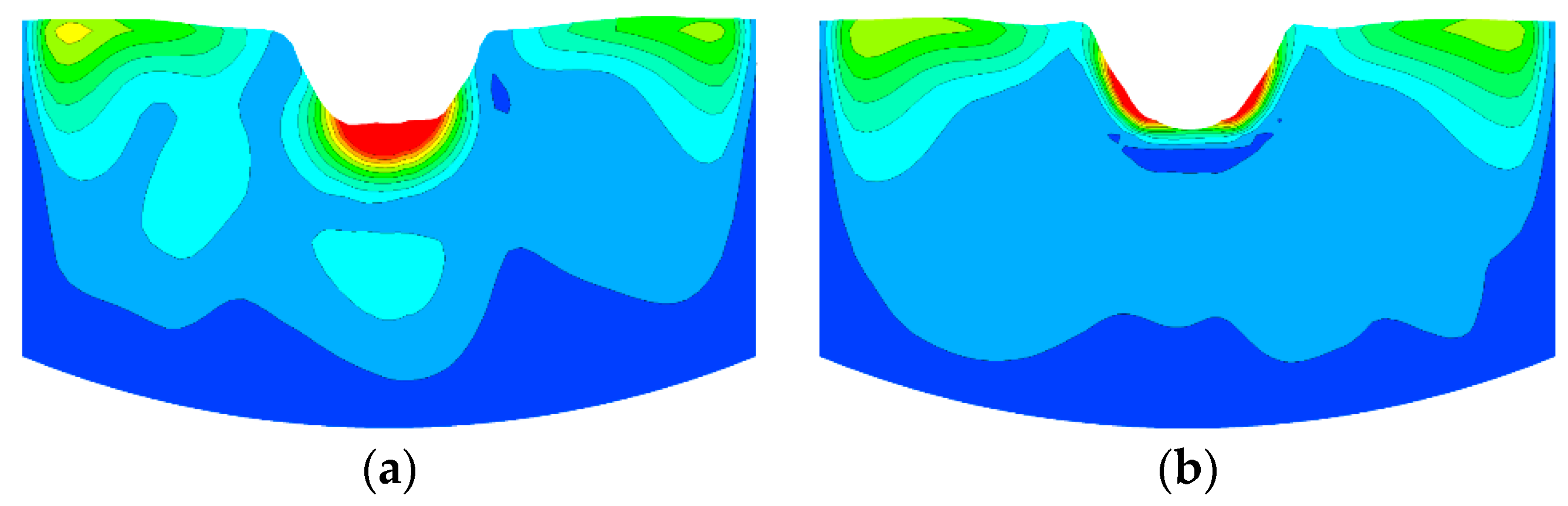
The mixing time was obtained by calculating the species transport Equation (10), which relates to the turbulent viscosity and flow field. The tracer mixing has two type, one is convection expressed as , the other is diffusion expressed as . The is mainly related to the flow field and the is mainly related to the turbulent viscosity expressed as . So, the mixing time calculated by Equation (10) is determined by turbulent viscosity and flow field. Figure 8 showed a comparison of the simulated results of mean turbulent viscosity (μt) distributions using a swirler lance and a non-swirler lance. The results indicated that the μt is larger when using a swirler lance, which may promote both the convective mixing and the diffusion mixing of tracer.
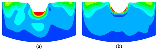
Figure 8.
Simulated results of mean turbulent viscosity distributions. (a) With a swirler and (b) without a swirler.
3.3. Effect of the Lance Diameter on Mixing Time
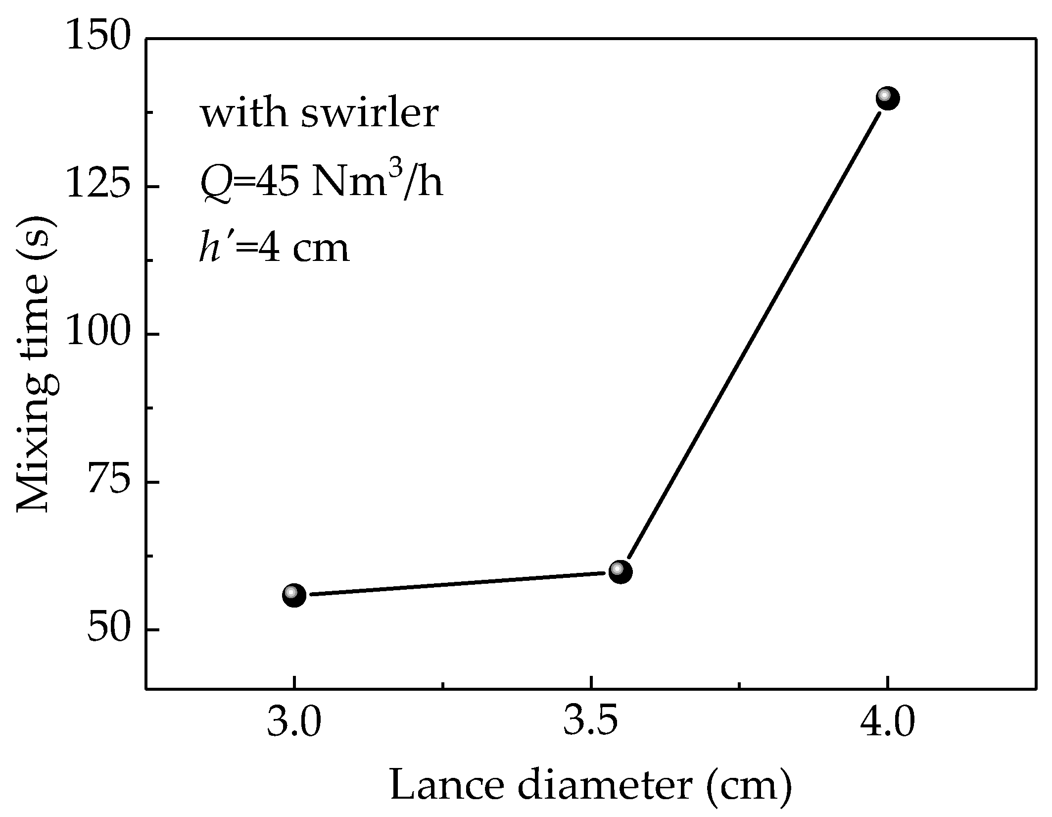
Figure 9 illustrates the effect of the change in the diameter of a lance equipped with a swirler on the mixing time at a gas flow rate (Q) of 45 Nm3/h and lance submergence depth of 4 cm. The figure clearly indicates that the mixing time increases with the lance diameter. With increases in the lance diameter, the gas velocity at the lance outlet decreases leading to a small turbulent viscosity and lower liquid velocity that causes weaker stirring in the bath, which eventually extends the mixing time. On the other hand, the splashing is increased when using a lance with a small diameter. Therefore, the lance diameter must be optimized to maintain high mixing efficiency and low surface splashing.

Figure 9.
Simulated results of the relationship between mixing time and lance diameter.
3.4. Effect of Gas Flow Rate on Mixing Time
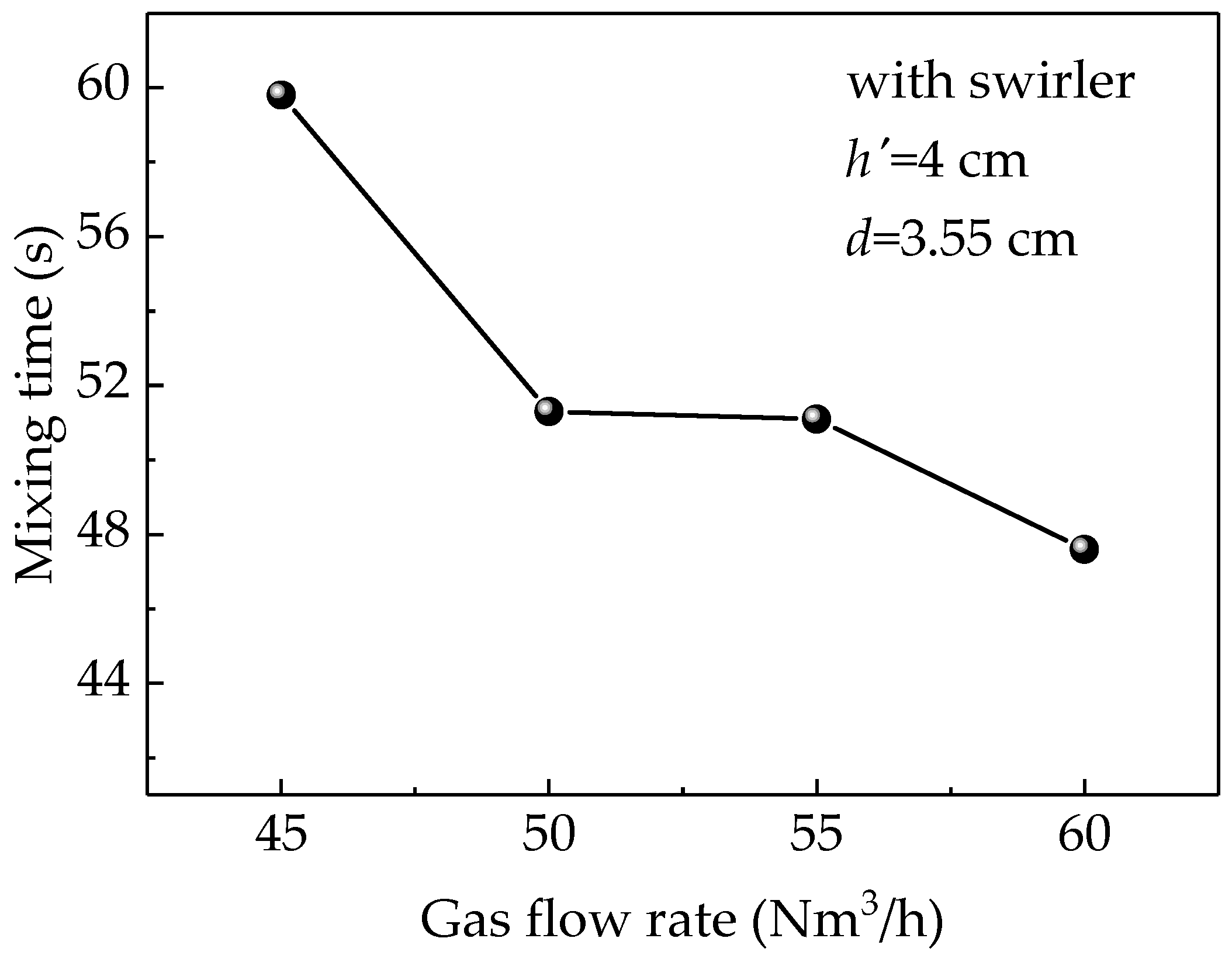
Figure 10 shows the effect of gas flow rate on the mixing time at the submerged depth of 4 cm with a Φ3.55 cm-lance equipped with a swirler. The figure indicates that the mixing time is inversely related to the gas flow rate because increasing the gas flow rate increases the kinetic energy. However, when gas flow rate was between 50 and 55 Nm3/h, there was a little variation in the mixing time, while the decreasing trend became clearer when the rate exceeded 55 Nm3/h. Although the mixing time was the reduced, large gas flow rates produce large splashes, which limits the ability to use higher gas flow rates to reduce mixing time. Therefore, 50 Nm3/h could be considered the optimal gas flow rate when the splash is not large.

Figure 10.
Simulated results of the effect of different gas flow rates on the mixing time.
4. Conclusions
In this study, a two-phase, top-blown ISASMELT furnace model that uses CFD to calculate species diffusion was developed. In addition, a water model was built using a 1:10 scale to verify the reliability of numerical simulation by experimentally measuring the mixing time. The comparison results indicate that the mixing time measured using the two methods exhibited similar trends. Moreover, the effects of lance diameter, lance submergence depth, gas flow rate, and the presence of swirlers on the mixing time were studied. The following conclusions can be drawn from the study:
(1) The mixing time is mainly determined by the turbulent viscosity and flow field. When using a lance with a swirler, both the convective mixing and the diffusion mixing of tracer were promoted due to the high turbulent viscosity that was obtained, and turbulent flow field can accelerate the species diffusion.
(2) The lance diameter should not be too large, and ideally should be kept smaller than 3.55 cm, because, at a fixed gas flow rate, the gas injected velocity decreases with the increase in lance diameter. So, the mixing energy, which depends on the gas velocity, may decrease rapidly.
(3) Meanwhile, optimal mixing time with low splashing can be obtained at a gas flow rate of about 50 Nm3/h, lance diameter of 0.035 mm, and a lance submergence depth of 0.04 m when using a swirler lance.
Author Contributions
Conceptualization, H.Z.; writing—original draft preparation, T.L.; formal analysis, P.Y.; investigation, L.M.; supervision, F.L.
Funding
This research was funded by the National Natural Science Foundation of China, grant number 51504018 and the Fundamental Research Funds for the Central Universities, grant number FRF-TP-17-038A2.
Conflicts of Interest
The authors declare no conflict of interest.
References
- Huda, N.; Naser, J.; Brooks, G.; Reuter, M.; Matusewicr, R. CFD modeling of gas injections in top submerged lance smelting. In Proceedings of the 138th TMS Annual Meeting and Exhibition, San Francisco, CA, USA, 15–19 February 2009; The Minerals, Metals & Materials Society: Warrendale, PA, USA, 2009; Volume 2, pp. 95–102. [Google Scholar]
- Zhang, H.L.; Zhou, C.Q.; Bing, W.U. Numerical simulation of multiphase flow in a Vanyukov furnace. J. S. Afr. I. Min. Metal. 2015, 115, 457–463. [Google Scholar] [CrossRef]
- Ma, J.; Sun, Y.S.; Li, B.W. Spectral collocation method for transient thermal analysis of coupled conductive, convective and radiative heat transfer in the moving plate with temperature dependent properties and heat generation. Int. J. Heat Mass Tran. 2017, 114, 469–482. [Google Scholar] [CrossRef]
- Ma, J.; Sun, Y.S.; Li, B.W. Simulation of combined conductive, convective and radiative heat transfer in moving irregular porous fins by spectral element method. Int. J. Therm. Sci. 2017, 118, 475–487. [Google Scholar] [CrossRef]
- Nakanishi, K.; Szekely, J.; Chang, C.W. Experimental and theoretical investigation of mixing phenomena in the RH—Vacuum process. Ironmak. Steelmak. 1975, 2, 115–124. [Google Scholar]
- Lang, S.; Cui, Z.; Ma, X.; Rhamdhani, M.A.; Zhao, B.J. Mixing Phenomena in a Bottom Blown Copper Smelter: A Water Model Study. Metall. Mater. Trans. B 2015, 46, 1218–1225. [Google Scholar] [CrossRef]
- Zhao, H.L.; Zhang, L.F.; Yin, P.; Wang, S. Bubble motion and gas-liquid mixing in metallurgical reactor with a top submerged lance. Int. J. Chem. React. Eng. 2017, 15, 1–8. [Google Scholar] [CrossRef]
- Zhao, H.L.; Yin, P.; Zhang, L.F.; Wang, S. Water model experiments of multiphase mixing in the top-blown smelting process of copper concentrate. Int. J. Min. Met. Mater. 2016, 23, 1369–1376. [Google Scholar] [CrossRef]
- Schwarz, M.P.; Koh, P.T.L. Numerical modelling of bath mixing by swirled gas injection. In Proceedings of the SCANINJECT IV: 4th International Conference on Injection Metallurgy, Luleå, Sweden, 11–13 June 1986; MEFOS: Lulea, Sweden, 1986. [Google Scholar]
- Taylor, I.F.; Dang, P.; Schwarz, M.P.; Wright, J.K. An improved method for the experimental validation of numerical mixing time predictions. In Proceedings of the 1989 Steelmaking Conference Proceedings, Chicago, IL, USA, 2–5 April 1989; ISS/AIME: Chicago, IL, USA, 1989; pp. 505–516. [Google Scholar]
- Dang, P.; Schwarz, M.P. Simulation of mixing experiments in cylindrical gas-stirred tanks. In Proceedings of the 4th International Symposium on Transport Phenomena in Heat and Mass Transfer, University of New South Wales, Sydney, Australia, 14–19 July 1991; pp. 642–653. [Google Scholar]
- Livoic, P.; Rudman, M.; Liow, J.L. Numerical Modelling of Free Surface Flows in Metallurgical Vessels. App. Math. Modelling 2002, 26, 113–140. [Google Scholar] [CrossRef]
- Pan, Y.H.; David, L. Physical and mathematical modeling investigations of the mechanisms of splash generation in bath smelting furnaces. In Proceedings of the Seventh International Conference on CFD in the Minerals and Process Industries, Trondheim, Norway, 21–23 June 2011; CSIRO: Melbourne, Australia, 2011; pp. 9–11. [Google Scholar]
- Huda, N.; Naser, J.; Brooks, G.; Reuter, M.A.; Matusewicz, R.W. CFD modeling of swirl and nonswirl gas injections into liquid baths using top submerged lances. Metall. Mater. Trans. B 2010, 41, 35–50. [Google Scholar] [CrossRef]
- Zhu, M.Y.; Sawada, I.; Yamasaki, N.; Hsiao, T. Numerical simulation of three-dimensional fluid flow and mixing process in gas-stirred ladles. ISIJ Int. 1996, 36, 503–511. [Google Scholar] [CrossRef]
- Lee, K.S.; Yang, W.O.; Park, Y.G.; Yi, K. Fluid flow and mixing behavior in gas stirred ladle with submerged lance. Met. Mater. 2000, 6, 461–466. [Google Scholar] [CrossRef]
- Wang, S.B.; Wang, H.; Xu, J.X.; Zhu, D.F.; Sun, H.; Li, H.J. Hot-state numerical simulation study on top-blown bath in ISA furnace. Adv. Mater. Res. 2011, 383–390, 7406–7412. [Google Scholar] [CrossRef]
- Ramírez-Argáez, M.A. Numerical simulation of fluid flow and mixing in gas-stirred ladles. Mater. Manuf. Process. 2007, 23, 59–68. [Google Scholar] [CrossRef]
- Wang, Y.N.; Vanierschot, M.; Cao, L.L.; Cheng, Z.F.; Blanpaina, B.; Guo, M.X. Hydrodynamics study of bubbly flow in a top-submerged lance vessel. Chem. Eng. Sci. 2018, 192, 1091–1104. [Google Scholar] [CrossRef]
- Adib, M.; Ehteram, M.A.; Tabrizia, H.B. Numerical and experimental study of oscillatory behavior of liquid surface agitated by high-speed gas jet. App. Math. Modelling 2018, 62, 510–525. [Google Scholar] [CrossRef]
- Zhang, Q.; Yong, Y.; Mao, Z.S.; Yang, C.; Zhao, C.J. Experimental determination and numerical simulation of mixing time in a gas–liquid stirred tank. Chem. Eng. Sci. 2009, 64, 2926–2933. [Google Scholar] [CrossRef]
- Jahoda, M.; Tomášková, L.; Moštěk, M. CFD prediction of liquid homogenisation in a gas–liquid stirred tank. Chem. Eng. Res. Des. 2009, 87, 460–467. [Google Scholar] [CrossRef]
- Stapurewicz, T.; Themelis, N.J. Mixing and mass transfer phenomena in bottom-injected gas–liquid reactors. Can. Metall. Quart. 1987, 26, 123–128. [Google Scholar] [CrossRef]
- Geng, D.Q.; Lei, H.; He, J.C. Optimization of mixing time in a ladle with dual plugs. Int. J. Min. Met. Mater. 2010, 17, 709–714. [Google Scholar] [CrossRef]
- Li, L.; Liu, Z.; Li, B.; Matsuura, H.; Tsukihashi, F. Water model and CFD-PBM coupled model of gas-liquid-slag three-phase flow in ladle metallurgy. ISIJ Int. 2015, 55, 1337–1346. [Google Scholar] [CrossRef]
- Maldonadoparra, F.D.; Ramirezargaez, M.A.; Conejo, A.N.; Gonzalez, C.A. Effect of both radial position and number of porous plugs on chemical and thermal mixing in an industrial ladle involving two phase flow. ISIJ Int. 2012, 51, 1110–1118. [Google Scholar] [CrossRef]
- Nilmani, M.; Conochie, D.S. Gas Dispersion with swirled lances. In Proceedings of the 4th International Conference on Injection Metallurgy: Scaninject IV, Luleå, Sweden, 11–13 June 1986; MEFOS: Lulea, Sweden, 1986. [Google Scholar]
- Neven, S.; Blanpain, B.; Wollants, P. Injection dynamics in an Isasmelt reactor. In Proceedings of the EPD Congress 2002, Seattle, WA, USA, 17–21 February 2002; The Minerals, Metals & Materials Society: Seattle, WA, USA, 2002; pp. 449–459. [Google Scholar]
- Yokoya, S.; Takagi, S.; Iguchi, M.; Marukawa, K.; Hara, S. Formation of fine bubble through swirling motion of liquid metal in the metallurgical container. ISIJ Int. 2000, 40, 572–577. [Google Scholar] [CrossRef]
© 2019 by the authors. Licensee MDPI, Basel, Switzerland. This article is an open access article distributed under the terms and conditions of the Creative Commons Attribution (CC BY) license (http://creativecommons.org/licenses/by/4.0/).