Predicting the Tensile Behaviour of Cast Alloys by a Pattern Recognition Analysis on Experimental Data

Abstract

The ability to accurately predict the mechanical properties of metals is essential for their correct use in the design of structures and components. This is even more important in the presence of materials, such as metal cast alloys, whose properties can vary significantly in relation to their constituent elements, microstructures, process parameters or treatments. This study shows how a machine learning approach, based on pattern recognition analysis on experimental data, is able to offer acceptable precision predictions with respect to the main mechanical properties of metals, as in the case of ductile cast iron and compact graphite cast iron. The metallographic properties, such as graphite, ferrite and perlite content, extrapolated through macro indicators from micrographs by image analysis, are used as inputs for the machine learning algorithms, while the mechanical properties, such as yield strength, ultimate strength, ultimate strain and Young’s modulus, are derived as output. In particular, 3 different machine learning algorithms are trained starting from a dataset of 20–30 data for each material and the results offer high accuracy, often better than other predictive techniques. Concerns regarding the applicability of these predictive techniques in material design and product/process quality control are also discussed.

1. Introduction

An accurate knowledge of the mechanical properties of materials represents the first step towards their correct use in any field of engineering and in everyday life. Thanks to this information, for instance, it is possible to design structures and components in order to optimize their functionality according to technical parameters of specific interest such as strength, weight, safety, costs and so forth [1,2,3,4].

In the case of metals and, especially, of rather common cast irons [5,6,7], the shared opinion is that their properties are quite predictable (e.g., fatigue [8], abrasion [9], fracture [10], strength [11]).

This is certainly the case when compared to other families, such as organic or composite materials. It is also possible to say that everything depends on the perspective. Since metals are widely known and used, low unpredictability in their properties is expected but actually quite common metal alloys, such as cast irons, can be affected by a not negligible variability in their essential properties [12,13].

From the constituent elements to the process parameters, a large list of factors can interfere with the microstructures of an alloy and, as a consequence, on its properties [14,15].

Although some uncertainties could be easily eliminated (e.g., better control on stoichiometry), it is not so simple in reality. In a traditional foundry, for instance, up to 30% of the metal originates from reused materials, with great advantages in terms of costs and environmental protection [16] but risks in controlling the chemical composition and a certain variability in the cast alloy properties [17].

This variety is the reason for the prevalence of cast iron throughout history and in the present [18]. Grey, white, malleable or ductile—cast alloys can provide largely different properties, offering a valid choice of materials in dissimilar situations. With minimal changes to the composition (e.g., from 3% to 4% in the carbon content) or the use of additives in marginal quantities (<1%), properties such as tensile strength move from 170 to 930 MPa, elongation from 0.5 to 18% and hardness from 130 to 450 HB [19].

This versatility is a weakness when constancy in the material’s property is necessary. In Reference [20] it is reported, for instance, that a relevant change in the microstructure and in the mechanical properties of a grey cast iron extracted from identical sand-cast parts produced by different foundries.

In this study, which starts from an extensive experimental test session (with data published in References [21,22,23]), it can be observed that two successive metal fusions, carried out a few hours later and without voluntary changes in the process parameters, lead to slightly different metallographic profiles between them. Furthermore, specimens extracted from the same casting, although they come from almost identical metal casting conditions, then take on a slight difference in metallographic terms, probably linked to different cooling conditions. These are all rather common knowledge in foundries that, however, lead to an intrinsic variability in the properties of the materials to be considered in the product design and, even, in the process designs.

This study intends to take a further step. Given that it is not possible to reduce the variability in mechanical properties as much as desired, a valid way of predicting them is sought.

Commonly, the mechanical properties of cast irons are related to their metallurgical ones, as reported in the case of Reference [24], which is especially focused on the latest research in solidification and melt treatments. It means, in practice, that micrographs are analysed with the scope to develop models and predictive formulae. A valid example of the current situation is represented by Reference [25], research concerned with the ability of the main theories to predict the fatigue limit of nodular cast iron. It reintroduces several previous studies dealing with the effect of small defects, such as micro-shrinkage cavities or pores and graphite nodules (shape and size) and with the characteristic of a microstructure. At the same time, it also highlights scarce applicability of the existing models and proposes a new correlation in the prediction of the fatigue limit, which involves additional parameters.

Other investigations proposed passing by the overall aspects, and representing the materials that are detectable from micrographs, such as content of graphite, ferrite, perlite, the grade of nodularity, vermicularity and so on (e.g., Reference [26]). Unfortunately, there is no direct connection between one of those characteristics and its mechanical properties and their relationship is hidden behind mutual interactions.

For this reason, recently studies have been successfully proposed to predict the mechanical characteristics of cast alloys by exploiting artificial intelligence approaches (as in References [27,28,29]).

The list of methods and tools to make concrete a general concept for Artificial Intelligence (AI) is enormous, rapidly evolving and cannot be disclosed in a few words [30]. However, one of the fundamental principles underlying the application of AI to material engineering, including prediction, is to use its ability for ‘pattern recognition’ [31].

An AI algorithm can be built to recognize patterns (such as recurrences, schemes, similarities) that the human mind cannot. This happens when, as in our case, the patterns are hidden on multiple levels. For instance, the ductility of cast iron—able to double the yield strength in the alloy, an interesting property for its real uses—can be provided by graphite in the form of very tiny nodules [32], together with a specific range of ferrite and pearlite content [33]. This metallurgical situation is obtained only by merging different conditions as (between the others) a specific range in magnesium content and a restricted addition of cerium and different temperatures [34].

While it is objectively complex to develop mathematical models to predict the properties of materials taking into account the combination of several factors, it is relatively simple to use one of the many AI algorithms, accepting a given approximation in its predictions [35].

This is certainly determined by the fact that AI algorithms, even rather complex ones, are now available to everyone and, at the same time, they offer high quality results. It depends on the positive combination of the mentioned pattern recognition with the concept of ‘machine learning’ (ML), an application of AI that provides systems the ability to automatically learn and improve from experience without being explicitly programmed [36].

The process of learning begins with observations or data, such as examples, direct experience or instruction, in order to look for patterns in data and make better decisions in the future based on this information [37].

This process can be implemented according to one of several different AI strategies, commonly categorized as “supervised,” “semi-supervised,” “unsupervised” or “reinforcement” machine learning.

In the first case, the dataset of information (input) is provided together with the results (output). The algorithm uses these data to learn the relations existing between inputs and outputs. When finished, it is ready to propose an output per each new set of input values [38].

In the second category—“unsupervised”—the ML process means that there is no distinction between input and output: each set of values is considered as an input and the algorithm is forced to find patterns without a specific external base of information [38].

Semi-supervised learning methods are something in between the other two categories: there is some form of feedback available for each step or action but there is no label or error message [38].

Finally, the reinforcement learning method interacts with its environment by producing actions and discovers errors or rewards [38]. Trial and error search and delayed reward are the most relevant characteristics of reinforcement learning.

Since ML enables the analysis of massive quantities of data, these learning methods often benefit from a data analysis process called “clustering,” introduced with the scope of grouping similar entities. It helps to profile the attributes of different groups, giving insight into their different underlying patterns [39,40]. The clustering analysis is also used to reduce the dimensionality of information with respect to the data characterized by a large number of variables. Between other algorithms for clustering, probably the most popular in ML are K-mean Clustering and Hierarchical Clustering.

Even if the unsupervised algorithms are quite uncommon in general and even less common in the fields of mechanical and material engineering, they are presented here since they seem ready to revolutionise investigations of the real world [36,37,38,39,40]. These advanced methods, in fact, can learn without passing for a conventional procedure of ML, based on specific datasets. They simply apply rules and learn by mistakes, following a system of evaluation of potential solutions based on scores [41].

Regardless of the ML technique, the success in prediction depends on the capability of each method to structure information acting on different levels. Supervised learning is useful in cases where a property (label) is available for a particular dataset (training set) but is missing and should be predicted for other cases. Unsupervised learning is used to detect implicit relationships in a given unmarked dataset.

In the case of material properties, as mentioned, the complexity can be related to the fact that these properties are connected with each other and to other chemical-physical ones, in a skein of relations that has to be untied before predictions. Machine Learning comes to the rescue because it allows the unhooking of the intermediate levels (“hidden”) from the superficial levels so that these first ones can be configured in full freedom in the search for correlations (pattern recognition). This process allows the collection of the input of a first level of knowledge to transform it into the output of a second level in an operation that always leads to abstracting of concepts. Learning takes the form of a pyramid with the highest concepts learned starting from the lowest levels [42].

It also means that, in the near future, an expert system can probably be installed in a foundry, monitoring the material/process situation but, at the moment, these systems are limited to a few very interesting research experiences. For instance, in Reference [43] an Artificial Neural Network (ANN) was used to classify nodular, grey or malleable cast irons on the basis of their microstructure. After a training session made by 60 samples, the AI showed an accuracy in selection very similar to that obtained by visual human tests. Reference [44] also deals with ductile cast iron and ANN methods; in particular, different networks were built and trained by 700 melts and used to predict tensile strength, elongation and hardness. In addition, in the same article, useful considerations are proposed regarding the ANN modelling and its input parameters, together with an assessment of their significance and availability in an industrial environment.

In brief, it is possible to say that an approach, based on AI and ML, can be conveniently used in material engineering [45,46]. Furthermore, the accuracy in prediction depends on several aspects, including the consistency and the quality of the data used for training.

2. Aims and Scope

This research has three main objectives, as follows:

-

Predict the mechanical properties of metals and, in particular, the tensile properties such as, yield strength, ultimate strength, ultimate strain and Young’s modulus, starting from experimental data. In addition, it would be possible to investigate the relationship between these properties and fundamental aspects of metallurgy, as in the cases of constituent elements, microstructures, process parameters or treatments.

-

Use information directly taken from micrographs by a conventional process of image analysis but globally converted into macro-indicators related to the content of graphite, ferrite, perlite, nodularity and vermicularity. In addition, it would be possible to discuss the interrelations existing between all these features—mechanical and metallurgical—with the scope to recognize essential and overabundant information. This investigation will involve two different families of cast alloys, a nodular cast iron (SGI) and a less common compact graphite cast iron (CGI).

-

Select and use these essential data inside a Machine Learning (ML) approach, based on pattern recognition, with the scope to perform an ‘intelligent analysis’ of experimental measures. In this task, some of the most common methods of ML will be applied, specifically the Random Forest (RF), the Artificial Neural Network (NN) and the k-nearest neighbours (kNN). These classifiers will be implemented by the use of conventional codes and accessible platforms, comparing them in terms of functionality and accuracy in prediction, especially in association with the consistency and quality of the dataset used for training but also considering the overall variability of the phenomena under investigation.

-

Introduce essential concerns regarding the real applicability of these techniques for scopes related to the material design, product/process quality control and so on, including practical suggestions on the way to simplify the procedure towards an industrially-oriented application.

3. Materials and Methods

3.1. Experimental Data

Measures were derived from a large experimental campaign undertaken in the past by some authors on foundry alloys, where samples in nodular iron and compact graphite cast iron were manufactured and mechanically characterized. These phases are detailed in References [21,22,23] and are here briefly summarized.

3.1.1. Casting

Samples were made by a traditional process of green sand moulding, using a hot blast long campaign cupola furnace [47], filled with layers of coke and ignited with torches. When the coke was very hot, solid pieces of metal were charged and alternated with additional layers of fresh coke. The high temperature, together with the other chemical conditions, transformed the solid metal into molten iron. Sand shapes were placed on the pouring line and, then, filled with molten iron.

According to the process parameters, including the use of inoculants, it was possible to produce two different cast alloys:

1)

Spheroidal Graphite Iron (SGI), a material also called nodular or ductile iron with respect to its high ductility, offered by the spheroidal shape of graphite;

2)

Compacted Graphite Iron (CGI), a material with intermediate properties between grey and nodular iron, thanks to a more compact form of graphite that is becoming quite popular, particularly in the automotive sector [48].

The castings were finally shaped by tool machining to extract samples in accordance with the experimental standards. In particular, 4 metal castings, manufactured on two different days, were created.

Extraordinary care was taken to minimize the risk of unexpected changes in the casting conditions, especially in terms of chemical composition, temperature and other process parameters that could interfere with the metallurgical stability (also in accordance with Reference [49]). For instance, the castings used for extracting samples were produced after a long time of conventional production in order to stabilize both temperature and metallurgy profiles. In addition, the chemical composition of the alloys was verified several times by off-line tests.

3.1.2. Metallurgical and Mechanical Properties

The ML algorithms were trained by experimental data from 48 samples, 27 in SGI and 21 in CGI. In particular, the following metallographic factors were used:

-

Quantity of Graphite

-

Quantity of Ferrite

-

Quantity of Perlite

-

Grade of Nodularity

-

Grade of Vermicularity

with the related values estimated (in%) by considerations of the micrographs. An image analysis was permitted to consider the presence and the geometry of the graphite inside the cast alloy (in terms of area, perimeter, Feret diameter and so on).

In addition, every set of metallographic characteristics was combined with related mechanical properties, as measured in accordance with the EN ISO 6892-1:2016 [50]:

-

Ultimate Tensile Strength [UTS],

-

Yield Strength [YS],

-

Ultimate Strain [ε],

-

Young’s modulus [E].

In synthesis, each one of these 48 samples provided a specific set of 5 (five) metallurgical and 4 (four) values, used in the machine learning. These data are available in

Table A1. Metallographic and mechanical properties of specimens in Spheroidal Graphite Iron (SGI). Data from [21,22,23].

Specimen	GR	FE	PE	NO	VE	UTS	YS	ε	E
	%	%	%	%	%	MPa	MPa	%	GPa
1	9.1	47.5	43.4	53.9	36.8	500.0	315.3	10.2	154.5
2	12.2	47.1	40.8	63.6	27.2	501.0	302.3	10.3	164.6
3	13.6	42.5	43.9	75.2	17.0	508.7	315.7	8.6	184.9
4	8.6	48.6	42.8	62.6	30.4	496.8	301.2	11.6	184.9
5	12.1	48.5	39.5	67.1	26.2	494.8	325.4	8.5	170.5
6	11.2	42.8	46.0	68.8	23.7	508.8	314.8	8.0	185.7
7	8.3	43.6	48.1	50.9	40.9	501.4	309.2	9.8	153.0
8	12.6	43.6	43.8	79.0	15.2	500.5	309.4	8.8	178.2
9	6.3	52.8	40.9	56.4	34.4	510.2	302.1	8.0	155.0
10	8.6	43.7	47.8	65.7	24.3	549.9	344.7	11.7	168.9
11	12.1	44.8	43.1	75.5	17.1	561.5	347.5	13.4	178.2
12	8.1	49.0	42.9	75.7	17.3	545.4	329.1	12.8	165.4
13	9.2	40.8	50.0	66.9	23.6	554.4	352.4	10.4	155.3
14	7.1	44.6	48.3	68.6	22.3	544.8	346.4	10.9	176.7
15	9.4	47.3	43.4	75.1	17.1	557.4	348.7	12.2	174.7
16	13.2	34.2	52.7	86.1	9.4	570.4	354.8	11.4	141.7
17	11.3	30.5	58.2	85.7	9.4	586.4	366.5	7.5	186.0
18	13.7	39.2	47.1	84.4	10.8	564.4	354.9	9.8	167.0
19	9.1	32.1	58.8	78.2	16.3	582.9	370.9	8.0	173.7
20	10.2	30.8	59.1	80.8	14.1	572.5	353.0	8.5	149.2
21	7.6	33.5	58.8	84.6	10.2	581.9	364.4	12.7	200.6
22	9.3	24.6	66.1	89.6	5.9	651.7	376.8	9.9	160.4
23	7.0	22.7	70.3	81.6	11.9	668.7	397.5	9.0	183.3
24	6.5	24.8	68.7	74.2	17.7	666.6	381.2	8.8	166.4
25	10.2	55.7	34.1	77.7	16.6	514.2	319.0	15.2	164.6
26	7.0	51.6	41.4	72.5	19.7	515.7	335.7	8.1	159.6
27	7.1	45.2	47.7	61.9	27.6	523.9	332.0	10.7	185.9
Mean (μ)	9.7	41.2	49.2	72.7	20.1	549.4	339.7	10.2	170.0
St. Dev. (σ)	2.3	9.0	9.4	10.2	8.8	50.6	26.7	1.9	13.9
R. St. Dev. (σ%)	24%	22%	19%	14%	44%	9%	8%	19%	8%

and

Table A2. Metallographic and mechanical properties of specimens in Compacted Graphite Iron (CGI). Data from [21,22,23].

Specimen	GR	FE	PE	NO	VE	UTS	YS	ε	E
	%	%	%	%	%	MPa	MPa	%	GPa
1	21.0	60.2	18.8	16.1	81.2	318.8	253.1	3.3	136.1
2	17.3	62.3	20.4	12.1	85.1	350.1	274.3	2.2	182.5
3	13.9	62.9	23.2	15.4	82.2	307.5	237.8	3.3	146.3
4	14.5	61.6	23.9	9.4	88.5	314.1	252.4	2.2	137.1
5	14.5	62.6	22.9	23.4	74.3	316.2	259.1	2.5	142.1
6	13.2	64.8	22.0	13.0	84.4	308.4	252.3	2.4	140.8
7	15.7	64.3	20.0	17.5	79.7	321.7	258.5	3.4	151.4
8	12.6	61.9	25.6	11.7	86.4	315.0	249.7	2.7	152.9
9	16.7	53.5	29.8	9.0	88.9	312.4	249.5	3.6	156.3
11	11.4	64.9	23.7	15.1	82.7	338.3	273.0	4.4	175.6
12	9.2	67.6	23.3	21.6	74.6	338.8	257.3	4.2	146.4
14	11.2	65.8	22.9	17.9	80.0	336.8	274.0	4.6	132.1
15	10.3	63.0	26.8	16.7	81.4	339.2	270.9	4.2	145.7
16	14.6	56.6	28.9	19.5	78.5	345.8	263.9	3.4	145.8
17	10.1	62.9	27.0	16.7	81.7	346.4	278.4	3.7	159.2
18	11.1	63.5	25.5	16.2	81.8	354.6	288.3	3.1	165.6
19	9.8	59.9	30.3	17.8	80.5	345.0	274.9	3.4	152.6
20	12.8	58.3	28.9	24.0	74.0	345.7	284.1	3.2	129.8
22	12.9	52.9	34.2	18.5	79.5	370.7	281.0	3.9	144.3
23	12.6	53.4	34.0	16.3	81.9	374.0	295.8	3.4	137.9
24	9.7	55.2	35.2	13.3	85.4	380.8	296.7	3.9	167.9
Mean (μ)	13.0	61.2	25.8	16.6	81.2	337.2	267.9	3.4	149.9
St. Dev. (σ)	3.0	4.3	4.7	4.0	4.2	21.8	16.3	0.7	14.0
R. St. Dev. (σ%)	23%	7%	18%	24%	5%	6%	6%	21%	9%

of Appendix B for SGI and CGI, respectively.

3.2. Machine Learning Algorithms

The current investigation was implemented by using the Orange program and its ML algorithms [51]. It is an open source platform for machine learning and data visualization, powered by 10 different algorithms, which can be used for data analysis and prediction.

In accordance with a quite common interpretation of the ‘No Free Lunch’ theorem [52], in the area of ML no universal method exists that can aprioristically provide the best results (for example, in terms of predictions) with respect to all sets of potential data [53]. In other terms, it is not possible to select the proper algorithm in advance.

In this research, in line with previous experiences where the ML has been applied to the prediction of metal properties [54], the analysis has been limited to the use of the following methods:

3.2.1. Random Forest (RF)

Random forest [55] is a popular algorithm of supervised learning, consisting of the use of a committee (ensemble) of decision trees. “Ensemble” means that it takes a bunch of “weak students” and combines them to form one strong predictor. “Weak students” are all random implementations of decision trees, which are combined to form a strong predictor—a random forest. The random forest method is often called the “improved implementation” of the decision tree method, because now to get a more accurate prediction and classification, not one tree is used but the tree committee. The method quickly gained popularity due to the comparative simplicity of setting up and running the analysis procedure. In contrast to the classical algorithms for constructing decision trees, in the random forest method, when constructing each tree, at the stages of splitting vertices, only a fixed number of randomly selected signs of the training set (the second parameter of the method) is used and a full tree is constructed (without cutting), that is, each leaf of the tree contains observations of only one class. A 15 tree, 32 fixed seed for a random generator was used, with a growth control based on the condition that no split was implemented for a subset smaller than 5 (

Table 1. Parameters of the Random Forest (RF).

Number of trees	15
Fixed seed for random generator	32
Do not split subset smaller than	5

).

3.2.2. Neural Network (NN)

A neural network [56] is another very popular algorithm of supervised learning. It is used to build an efficient encryption system using a constantly changing key. Neural networks offer a very powerful and general structure for representing a non-linear mapping of several input variables for several output variables. A neural network can be considered a suitable choice for functional forms used for encryption and decryption operations. The NN topology is an important issue, since the application of the system depends on it. Therefore, since the application is a calculation problem, a multi-layered topology was used. Neural networks offer a very powerful and general structure for representing a non-linear mapping of several input variables for several output variables. The process of determining the values of these parameters on the basis of a dataset is referred to as training and therefore the data set is usually referred to as a training set. A neural network can be considered a suitable choice for functional forms used for encryption and decryption operations. A neural network is a structure (network) consisting of a set of interconnected links (artificial neurons). Each link has a characteristic input / output and implements a local calculation or function. The output of any link is determined by the characteristics of its input / output, its relationship with other links, as well as external inputs, if any. A 5 layer neural network in backpropagation was used. The speed of learning was 0.6, the inertial coefficient was 0.5, the test mass tolerance was 0.02 and the tolerance of the learning set was 0.03 (

Table 2. Parameters of the Neural Network (NN).

Learning speed	0.6
Inertial coefficient	0.5
Test mass tolerance	0.02
Tolerance of the learning set	0.03
Number of layers	5

).

3.2.3. K-Nearest Neighbours (kNN)

The K-nearest neighbours method [57] is one of the methods for solving the classification problem. It is assumed that there is already some number of objects with an exact classification (i.e., for each of them it is known exactly which class it belongs to). It is necessary to work out a rule allowing the classification of a new object as one of the possible classes (the classes themselves are known in advance). At the heart of kNN is the following rule: an object is considered to belong to the class to which most of its closest neighbours belong. Under “neighbours” here are objects that are close to the studied in one sense or another. Note that here it is necessary to be able to determine how close objects are to each other, that is, be able to measure the “distance” between objects. This is not necessarily the Euclidean distance. This can be a measure of proximity of objects, for example, in colour, shape, taste, smell, interests, behaviour, and so forth. Consequently, to apply the kNN method in the feature space of objects, a certain metric must be introduced (that is, a distance function). If the nearest neighbours are divided into classes of approximately the same capacity, then, on the contrary, it makes sense to use those rules that take the distances into account to a greater degree (for example, the average rule). The rule of weighted majority takes into account both the number of objects in a class (via the weighting factor) and the distance to these objects. If there are a lot of classes and the weights are approximately the same, then first, such classes are selected so that their total weight is more than 0.5 and then one of the rules is applied. A Chebyshev metric was used with a number of neighbour equal to 2 and a uniform weight (

Table 3. Parameters of the k-nearest neighbours (kNN).

Metric	Chebyshev
Number of Neighbours	2
Weight	Uniform

).

3.3. Correlations

The existence of a link between the various variables under investigation was sought for by calculating the Pearson correlation index (as done in Reference [58]). Also called the linear correlation coefficient of Bravais-Pearson, this statistical index shows an eventual linear relationship between variables.

Given two statistical variables X and Y, the correlation index (r_xy) is defined as their covariance divided by the product of the standard deviations of the two variables. This index varies between −1 and +1, where a > 0 shows the two variables are directly correlated, a value of 0 is for variables are uncorrelated and, finally, <0 for variables are inversely correlated.

Moreover, for the direct correlation (and similarly for the inverse) it is distinguished:

• 0 < r_xy < 0.3 there is a weak correlation;
• 0.3 < r_xy < 0.7 there is a moderate correlation;
• r_xy > 0.7 there is a strong correlation.

The Pearson correlation was used in two alternative ways. It permitted relation of the:

-

experimental measures by way of estimating the influence between different properties;

-

experimental and predicted values by way of estimating the accuracy of the ML methods.

The adoption of the correlation coefficient as a way to evaluate the relationships between variables but also the accuracy in predictions was preferred in this study (similar to References [59,60]). Instead of other statistical approaches, it was considered for its extreme simplicity, both in terms of calculation and comprehension: the correlation coefficient directly represents a clear measure of the strength of the linear relationship between two variables. At the same time, it is useful to highlight that unrelated variables are not always independent: this depends on the fact that the correlation coefficient only detects a linear correlation.

4. Results

4.1. Experimental Measures

Table A3. Prediction of mechanical properties of Spheroidal Graphite Iron (SGI).

UTS				YS				ε				E
MPa	RF	NN	kNN	MPa	RF	NN	kNN	%	RF	NN	kNN	GPa	RF	NN	kNN
495	510	509	497	325	348	316	301	8.5	8.0	8.0	8.0	171	185	186	160
497	510	510	495	301	349	302	302	11.6	10.7	10.2	8.0	185	165	153	155
500	501	501	497	315	302	309	301	10.2	8.0	8.0	8.0	155	185	153	153
501	510	509	497	302	301	315	301	10.3	8.0	8.0	8.0	165	185	185	169
501	562	564	509	309	316	355	316	8.8	9.0	9.0	7.5	178	149	142	165
501	500	500	497	309	332	315	301	9.8	11.4	8.6	8.6	153	169	155	155
509	557	501	501	316	309	355	309	8.6	8.8	8.5	8.8	185	178	178	178
509	554	501	495	315	345	325	302	8.0	10.2	10.7	9.8	186	178	165	155
510	500	500	497	302	336	309	301	8.0	10.9	9.8	8.5	155	165	155	153
514	510	509	501	319	336	316	309	15.2	8.1	12.8	8.1	165	178	178	178
516	545	524	495	336	329	302	319	8.1	12.8	15.2	8.5	160	177	165	165
524	501	510	497	332	345	315	301	10.7	10.9	10.2	10.3	186	185	155	155
545	562	516	501	329	349	349	309	12.8	13.4	15.2	8.1	165	178	175	178
545	509	516	509	346	332	332	315	10.9	10.7	10.7	8.0	177	178	186	155
550	509	497	497	345	352	301	301	11.7	10.4	10.7	8.0	169	186	153	155
554	545	510	501	352	345	336	302	10.4	8.0	8.0	8.0	155	177	185	165
557	509	514	501	349	329	336	309	12.2	8.0	8.0	8.1	175	178	165	160
562	501	509	501	348	329	316	309	13.4	8.0	8.0	8.0	178	185	165	160
564	573	570	501	355	355	348	309	9.8	10.2	8.0	8.0	167	201	178	178
570	582	564	564	355	367	367	353	11.4	7.5	8.5	7.5	142	167	167	149
573	583	652	570	353	381	377	355	8.5	8.0	9.9	7.5	149	174	183	142
582	564	669	570	364	371	377	353	12.7	7.5	9.9	7.5	201	174	183	142
583	573	652	570	371	353	398	353	8.0	8.5	9.0	7.5	174	201	183	142
586	573	652	570	367	364	355	353	7.5	8.0	8.8	8.0	186	201	160	142
652	586	573	570	377	355	398	353	9.9	7.5	7.5	7.5	160	149	183	142
667	510	669	573	381	336	398	353	8.8	13.4	11.4	8.6	166	160	183	149
669	545	667	573	398	353	381	353	9.0	8.8	9.9	7.5	183	166	166	149

and

Table A4. Prediction of mechanical properties of Compacted Graphite Iron (CGI).

UTS				YS				ε				E
MPa	RF	NN	kNN	MPa	RF	NN	kNN	%	RF	NN	kNN	GPa	RF	NN	kNN
308	316	350	308	238	288	252	252	3.3	3.4	2.2	2.4	146	146	141	132
308	355	314	308	252	238	274	238	2.4	3.3	2.2	2.2	141	176	183	146
312	371	315	312	250	252	281	250	3.6	3.3	3.9	3.9	156	138	137	137
314	312	312	314	252	250	250	238	2.2	3.6	3.6	2.2	137	153	183	141
315	308	314	315	250	252	252	238	2.7	2.2	2.2	2.2	153	168	137	137
316	322	346	316	259	284	284	257	2.5	3.4	3.4	3.4	142	146	151	130
319	350	322	319	253	259	274	238	3.3	3.4	2.2	2.2	136	151	183	141
322	319	319	322	259	252	259	238	3.4	3.4	3.2	3.2	151	141	136	132
337	355	339	337	274	257	257	238	4.6	4.2	4.2	3.1	132	176	146	146
338	339	337	338	273	288	250	252	4.4	4.2	4.6	2.4	176	166	132	132
339	346	337	339	271	278	238	273	4.2	2.5	4.6	2.5	146	159	159	132
339	337	308	339	257	271	259	259	4.2	3.7	3.4	3.1	146	166	132	132
345	346	346	345	275	278	281	271	3.4	3.4	3.3	3.3	153	146	144	138
346	316	346	346	264	281	296	271	3.4	4.2	3.9	3.1	146	146	130	130
346	339	339	346	278	271	271	271	3.7	3.4	3.4	3.1	159	166	132	132
346	316	316	346	284	259	259	257	3.2	3.4	3.4	3.4	130	142	142	142
350	308	319	350	274	252	253	238	2.2	3.3	3.3	3.3	183	151	137	136
355	338	339	355	288	273	275	238	3.1	4.2	4.2	3.3	166	146	132	132
371	381	374	371	281	296	296	264	3.9	3.4	3.4	3.4	144	138	138	130
374	381	371	374	296	281	281	250	3.4	3.9	3.9	3.4	138	153	144	144
381	374	312	381	297	274	296	250	3.9	3.7	3.4	3.4	168	153	144	138

in Appendix C report the material tensile properties for SGI and CGI, respectively, as estimated by the three ML algorithms: Random Forest (RF); Neural Network (NN); k-Nearest Neighbours (kNN). Specifically, for each sample used in the experimental tests (48 in total), the expert system provided 3 different predictions (RF, NN, kNN) for each of the 4 mechanical properties under investigation (Ultimate Tensile Strength, Yield Strength, Ultimate Strain and Young’s modulus). These values are later considered and discussed in terms of Mean Values (μ), Variability (σ, σ_%) and Correlations (r_xy).

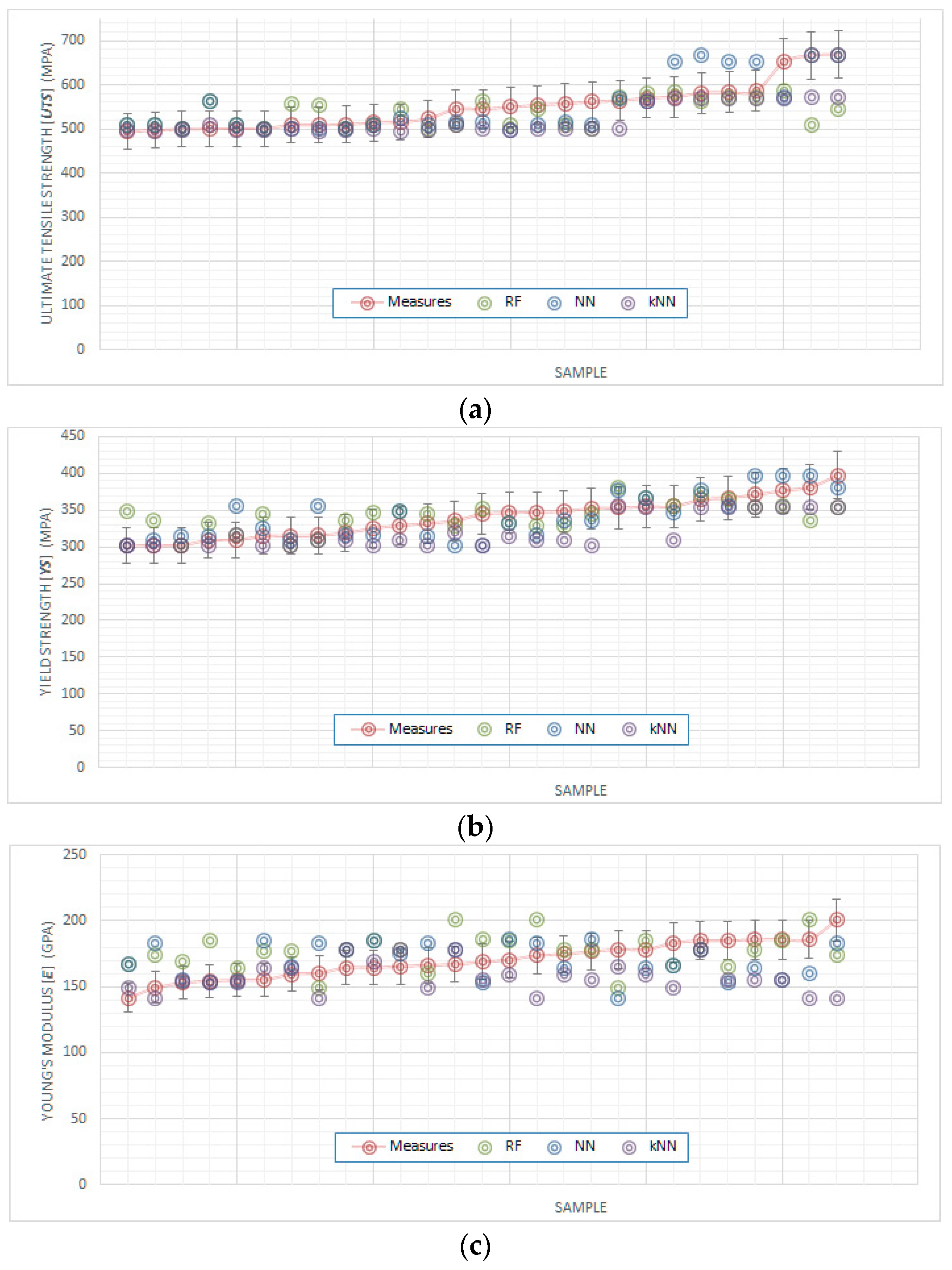
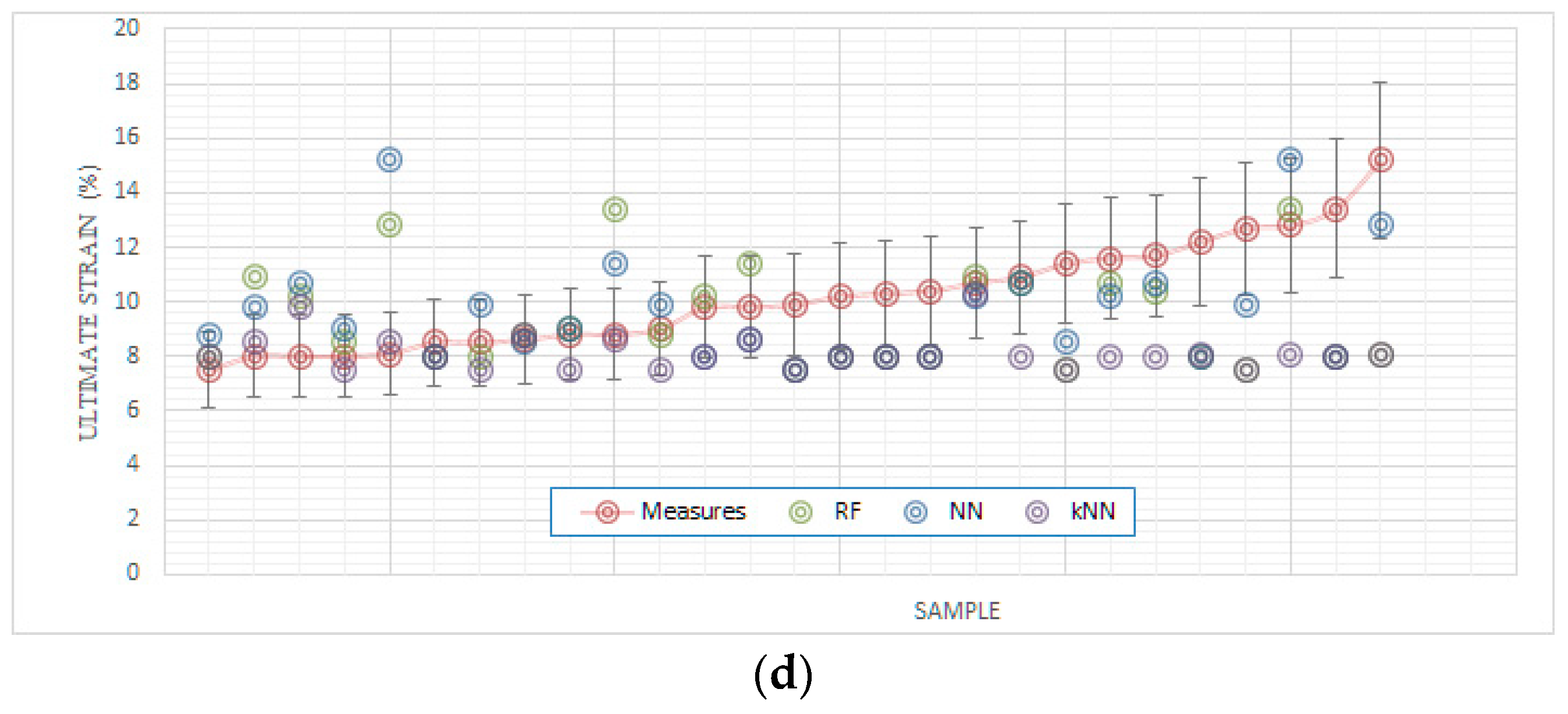
4.2. Spheroidal Graphite Cast Iron

In particular, the four diagrams in Figure 1 show these tensile properties in the case of SGI where the values from the measures are reported together with error bars representing the related variability. In addition, all the diagrams are displayed with a y-scale ranging from 0 to (approx.) the maximum value. These provide a visual representation of the ability of the ML methods to fit the experimental values. For instance, in the case of UTS, it is possible to see how the largest part of the predictions (specifically 69 on 27 × 3 = 81) falls inside the error bars (±9%). These error bars were evaluated starting from the experimental measures and passing by their relative standard deviation (σ_%). Per each property and each material, a specific σ_% can be defined and this percentage can be used for dimensioning the error bar. The related bars are intended to give an idea of the variability of the measures, showing at the same time how a large part of the predictions falls inside this variability.

Comparing these properties, it is also possible to recognize, in general, how prediction on UTS and YS seems better than those on ε and E.

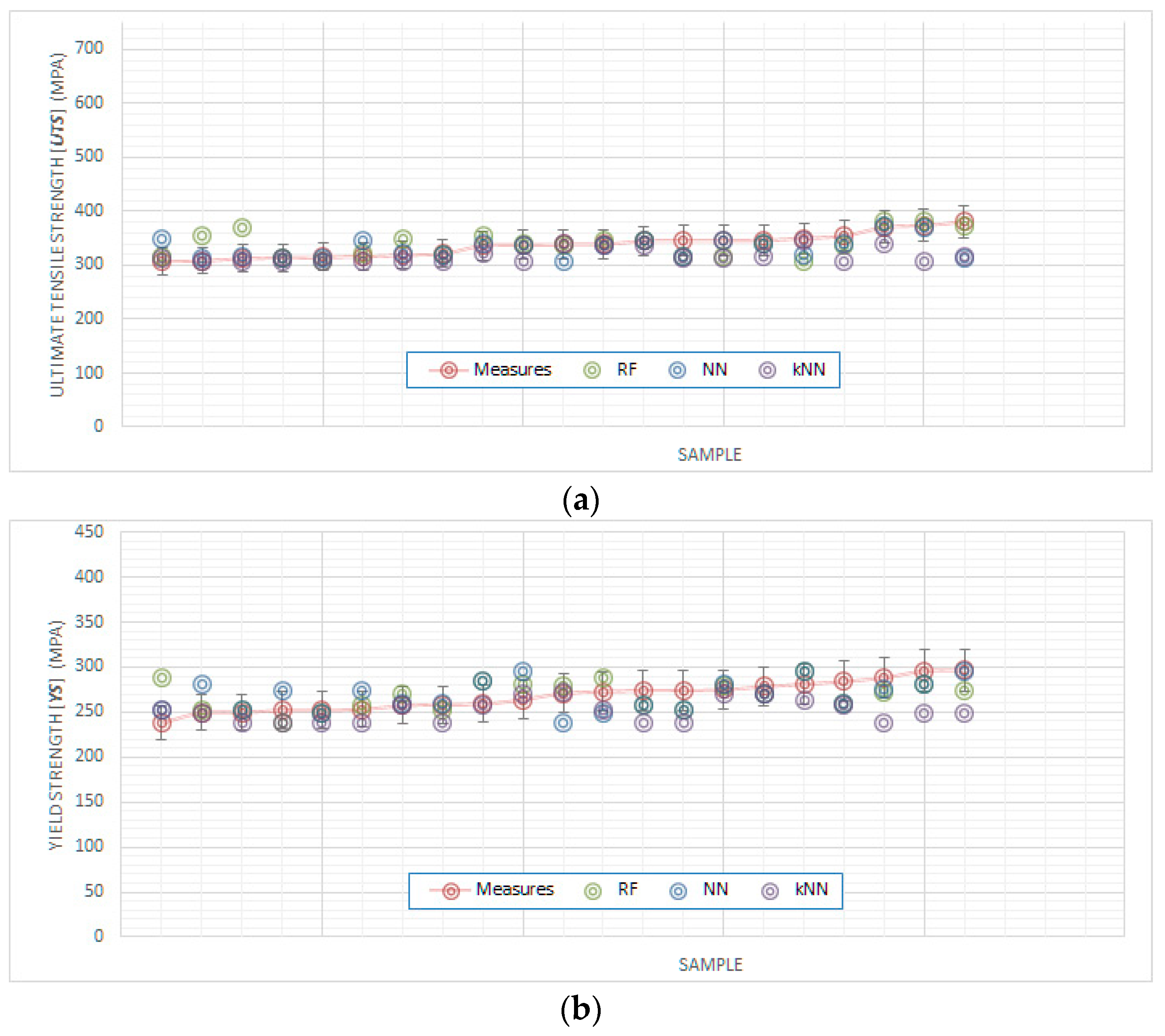
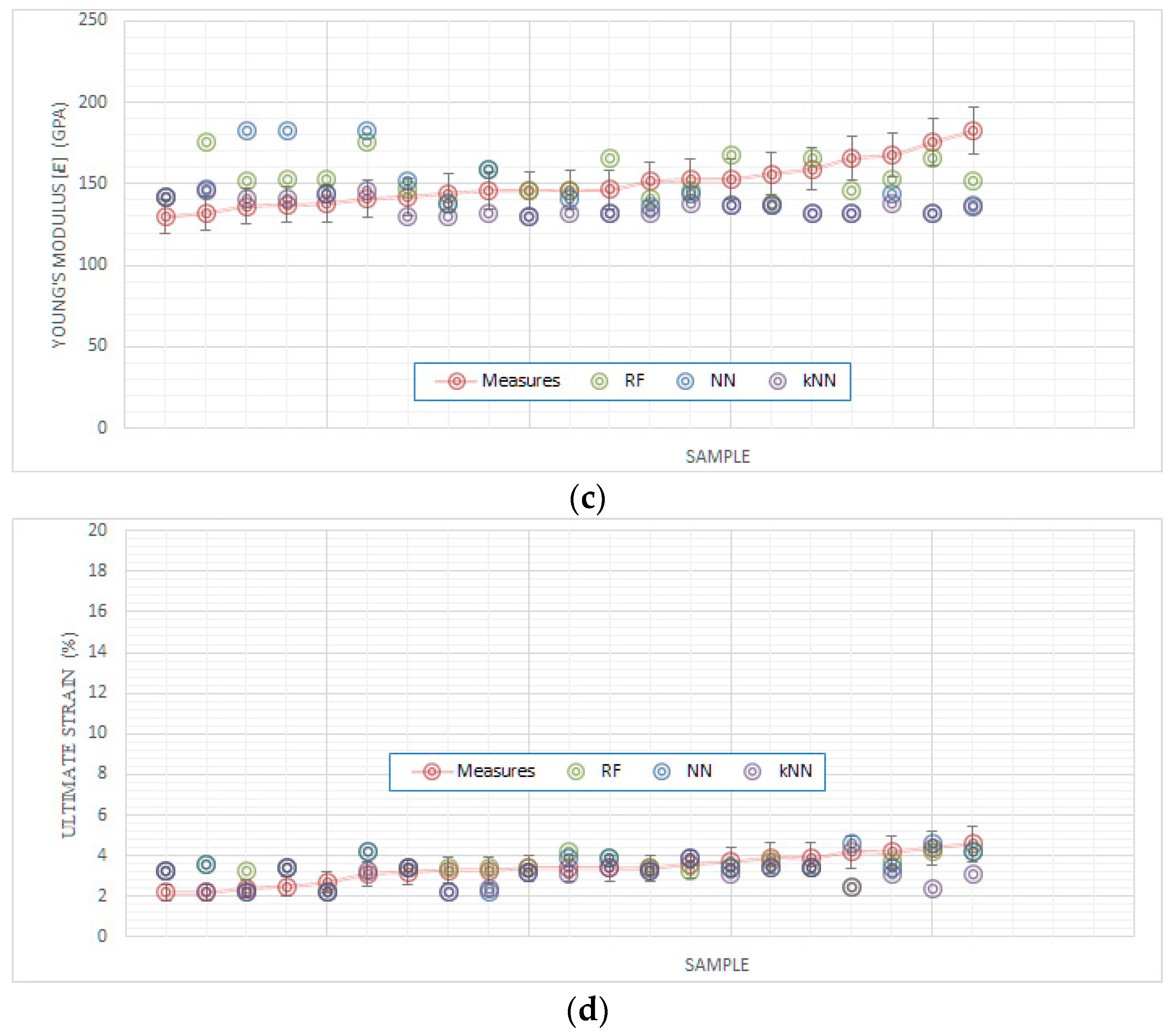
4.3. Compacted Graphite Cast Iron

The analogous diagrams in Figure 2 show the tensile properties for CGI. This analogy is also respected for considerations of data and evidence. For instance, also in this case for UTS, the major part of the predictions (specifically 16 values on 21 × 3 = 63) falls inside the error bars (±6%).

Finally, the diagrams are similarly scaled for Figure 1 and Figure 2, permitting a direct comparison between the properties of the two materials. It is evident, for instance, the lower properties of CGI respect to SGI.

5. Discussion

5.1. Prediction Model Validation

Before proceeding with discussing the results, it is appropriate to specify some additional concepts on the use of the learning and validation process within this work and justify them. Usually studies involving ML approaches divide the available data into two categories: those used for learning and those used for validating results. This apparently sensible and correct approach brings with it potential errors. For example, while the learning phase should vary slightly if information from a limited number of data is subtracted by the complete dataset, the validation phase is very sensitive to how many and which specific data are taken into account. Furthermore, whatever the result is, the doubt remains that the particular choice of data modified the general assessment on the validity of the entire prediction procedure.

This situation is frustrated when, as in the present case, external data are themselves subject to a high variability. In other words, it can be accepted that the expert system is trained with data subject to a certain intrinsic variability, waiting for its forecasts to be subject to a comparable variability. But, if these predictions are then compared with some specific data extracted from such a variable sample, the risk of making mistakes is rather high.

To avoid this risk, the simplest way is to increase the dataset of external data, to be used both for training and validating, as done in Reference [44]—where 700 samples were considered—all of them representing a homogeneous situation (same alloy, process conditions and so on). In the meantime, also considering the hypothesis where additional tests are not imaginable in short, a different approach was here proposed for data analysis. It is in line with another recent paper by some of the authors [54] where ML algorithms were used for the evaluation of the surface roughness evaluation in steel after thermal hardening by laser radiation. In brief, the validation is performed on the full dataset of values, not on part of it.

5.2. Data Preliminary Analysis

Considering the experimental measures, as reported in Appendix B in Table A1 and Table A2, it is clear there is a not marginal variability in values, in the cases of both metallurgical and mechanical properties.

The relative standard deviation (σ_%), expressed as the ratio between the standard deviation (σ) and the mean value (µ) permits a homogeneous comparison among parameters, providing useful information. For instance, in the case of SGI, the metallographic factors, expressed by σ_%, spread between 14% (nodularity) and 44% (vermicularity). This variability is lower but also relevant, in the case of CGI, limited between 5% (vermicularity) and 24% (nodularity). Also, in terms of mechanical properties, the same variability of measures is confirmed. In particular, it ranges from 5%–6% in the case of the Ultimate Tensile Strength and the Yield Strength of CGI, up to 19%–21% in the case of the Ultimate Strain of SGI for both alloys.

As a consequence, the complexity of using these data for predictions on material properties is evident. At the same time, in

Table 4. Correlation matrix between the metallurgical properties in the case of SGI and CGI.

SGI	Graphite	Ferrite	Perlite	Nodularity	Vermicularity
Graphite	1.00	0.04	−0.29	0.34	−0.30
Ferrite	0.04	1.00	−0.79	0.13	−0.19
Perlite	−0.29	−0.79	1.00	0.03	0.05
Nodularity	0.34	0.13	0.03	1.00	−0.99
Vermicularity	−0.30	−0.19	0.05	−0.99	1.00
CGI	Graphite	Ferrite	Perlite	Nodularity	Vermicularity
Graphite	1.00	−0.20	−0.45	−0.24	0.20
Ferrite	−0.20	1.00	−0.79	0.13	−0.19
Perlite	−0.45	−0.79	1.00	0.03	0.05
Nodularity	−0.24	0.13	0.03	1.00	−0.99
Vermicularity	0.20	−0.19	0.05	−0.99	1.00

the relationships between parameters, estimated by the Pearson correlation coefficient, is reported in the case of the metallurgical properties, showing that several parameters are, as weighted, in medium-strong relations (e.g., perlite vs ferrite or perlite vs graphite).

But the relations of real interest are those that can connect mechanical properties to the microstructural ones, in order to predict the overall behaviour of an alloy knowing its compound and microstructure. Several articles, as mentioned, move in that direction, relating micro- and macro-scales, while the current investigation limits its focus on data analysis.

In particular,

Table 5. Correlation matrix between the metallurgical and mechanical properties.

SGI	Graphite	Ferrite	Perlite	Nodularity	Vermicularity
Ultimate Tensile Strength (UTS)	−0.25	−0.87	0.90	0.63	−0.65
Yield Strength (YS)	−0.19	−0.83	0.84	0.67	−0.69
Ultimate Strain (ε)	−0.03	0.34	−0.32	0.05	−0.06
Young’s Modulus (E)	−0.03	−0.09	0.09	0.18	−0.21
CGI	Graphite	Ferrite	Perlite	Nodularity	Vermicularity
Ultimate Tensile Strength (UTS)	−0.44	−0.46	0.69	0.23	−0.17
Yield Strength (YS)	−0.46	−0.35	0.61	0.25	−0.17
Ultimate Strain (ε)	−0.47	0.00	0.29	0.28	−0.26
Young’s Modulus (E)	−0.11	0.08	0.00	−0.39	0.38

exhibits, in terms of Pearson correlation coefficients, the relationships between the metallurgical parameters and the mechanical properties.

Several preliminary considerations emerge from these data. According to the experimental values, as correlated by the Pearson coefficient, it seems that:

-

the SGI is more affected than the CGI with respect to changes in the metallurgical properties;

-

the content of graphite is not so relevant for the definition of mechanical properties, especially in the case of SGI, while it has a light negative effect on CGI;

-

the contents of ferrite and perlite, more than others, directly influence the material strength, especially in the case of SGI;

-

the ductility is directly related to ferrite and perlite content but not to graphite in the case of SGI, while the graphite shows a light negative effect on CGI;

-

the Young’s modulus, evaluated as standard, is practically uncorrelated, except for a slight dependency to the nodularity and to the vermicularity, more relevant in the case of CGI.

5.3. Expert Algorithms

This preliminary data analysis permits the presentation of a general situation, quite common in the strength of materials, where each material property seems to be related to many of the others without strong/predominant dependencies. The consequent network of weak correlations between properties makes the material data analysis complex. Thus, every approach searching for a linear dependency is almost useless, unable to “untangle the skein” and artificial intelligence can help with “cracking” this complexity.

An expert algorithm, in fact, can search for patterns to be recognized without considering their physical significance. It will simply scan data search for hidden analogies and structures, moving the vision between different levels of the knowledge abstraction.

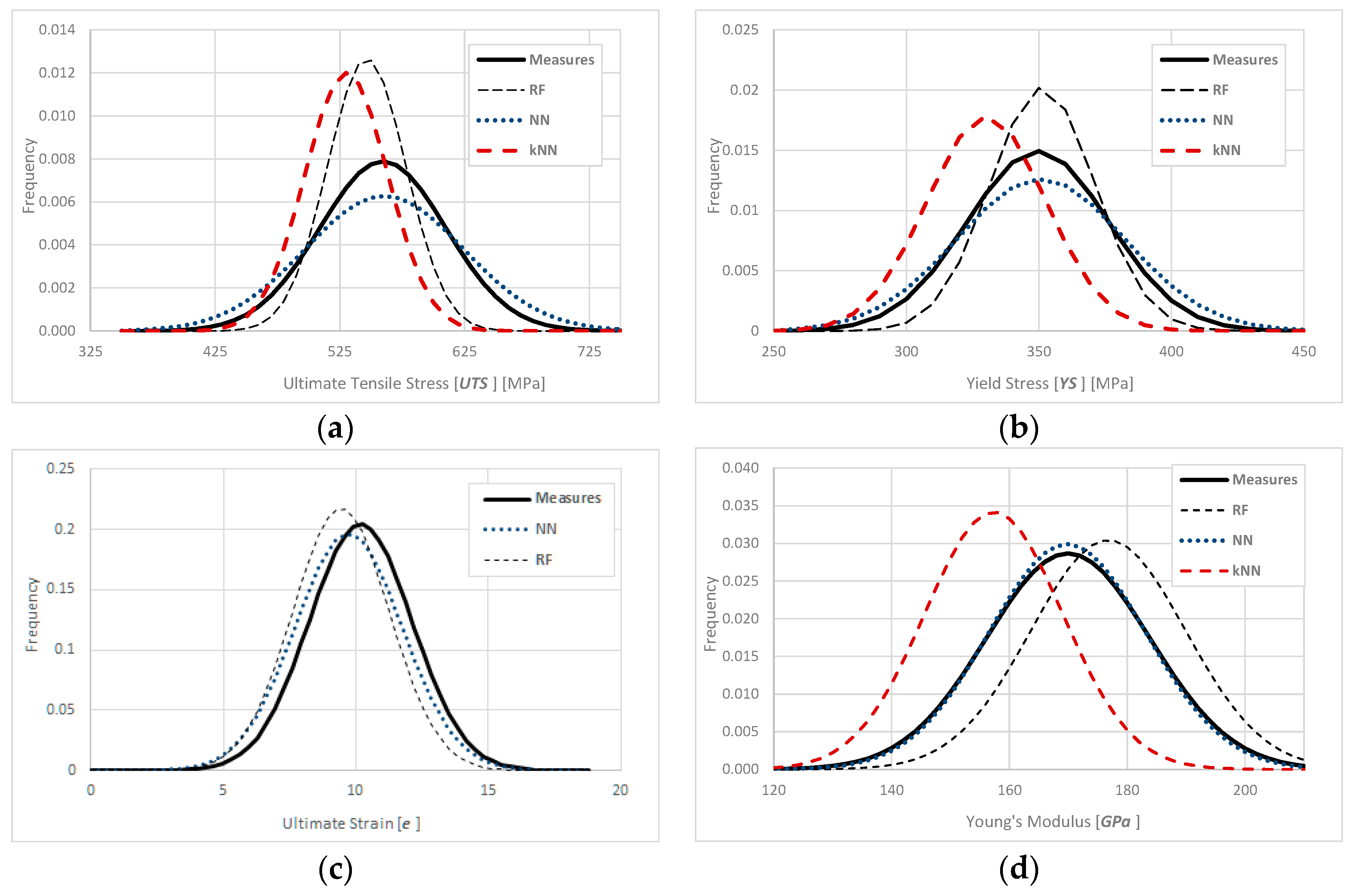
5.4. Mean Values and Variability

In

Table 6. Mechanical properties prediction in terms of mean values and standard deviations.

SGI	Unit	Data	RF	NN	kNN
Ultimate Tensile Strength (UTS)	MPa	549 ± 51 (9%)	536 ± 31 (6%)	550 ± 64 (12%)	520 ± 33 (6%)
Yield Strength (YS)	MPa	340 ± 27 (8%)	341 ± 20 (6%)	341 ± 31 (9%)	320 ± 22 (7%)
Ultimate Strain (ε)	%	10.2 ± 1.9 (19%)	9.4 ± 1.8 (19%)	9.7 ± 2.0 (21%)	8.1 ± 0.1 (8%)
Young’s Modulus (E)	GPa	170 ± 14 (8%)	177 ± 13 (7%)	170 ± 13 (8%)	157 ± 12 (7%)
CGI	Unit	Data	RF	NN	kNN
Ultimate Tensile Strength (UTS)	MPa	337 ± 22 (6%)	340 ± 24 (7%)	332 ± 19 (6%)	317 ± 5 (4%)
Yield Strength (YS)	MPa	268 ± 16 (6%)	268 ± 16 (6%)	268 ± 17 (6%)	251 ± 13 (5%)
Ultimate Strain (ε)	%	3.4 ± 0.7 (21%)	3.5 ± 0.5 (14%)	3.4 ± 0.7 (21%)	3.0 ± 0.5 (18%)
Young’s Modulus (E)	GPa	150 ± 14 (9%)	154 ± 12 (8%)	146 ± 17 (12%)	136 ± 20 (4%)

, the tensile properties for SGI and CGI are reported as predicted by the expert system, in terms of mean values and standard deviations. It is evident how the variability in predictions is in line with the initial variability of measures. For instance, the experimental data on SGI, measured on 27 specimens, show an average value of the UTS equal to μ = 549 MPa with variability a σ = ±51, equal to ±9%. Using these values, the three ML algorithms (RF, NN, kNN) propose three different predictions, equal to, in the mentioned case, respectively, 536 ± 31 (6%), 550 ± 64 (12%), 520 ± 33 (6%). The variability of those predictions (±6%; ±12%; 6%) is almost equivalent to the initial one (±9%). The same concept is also evident in the cases of all the other properties, demonstrating that the selected ML algorithms do not interfere with the base of data increasing its variability.

5.5. Mean Values and Error Estimation

In

Table 7. Error estimation in the prediction of mean values.

Property	SGI			CGI
	RF	NN	kNN	RF	NN	kNN
Ultimate Tensile Strength (UTS)	−2.4%	0.2%	−5.3%	0.9%	−1.5%	−5.9%
Yield Strength (YS)	0.3%	0.3%	−5.9%	0.0%	0.0%	−6.3%
Ultimate Strain (ε)	−7.8%	−4.9%	−20.6%	2.9%	−11.8%	−11.8%
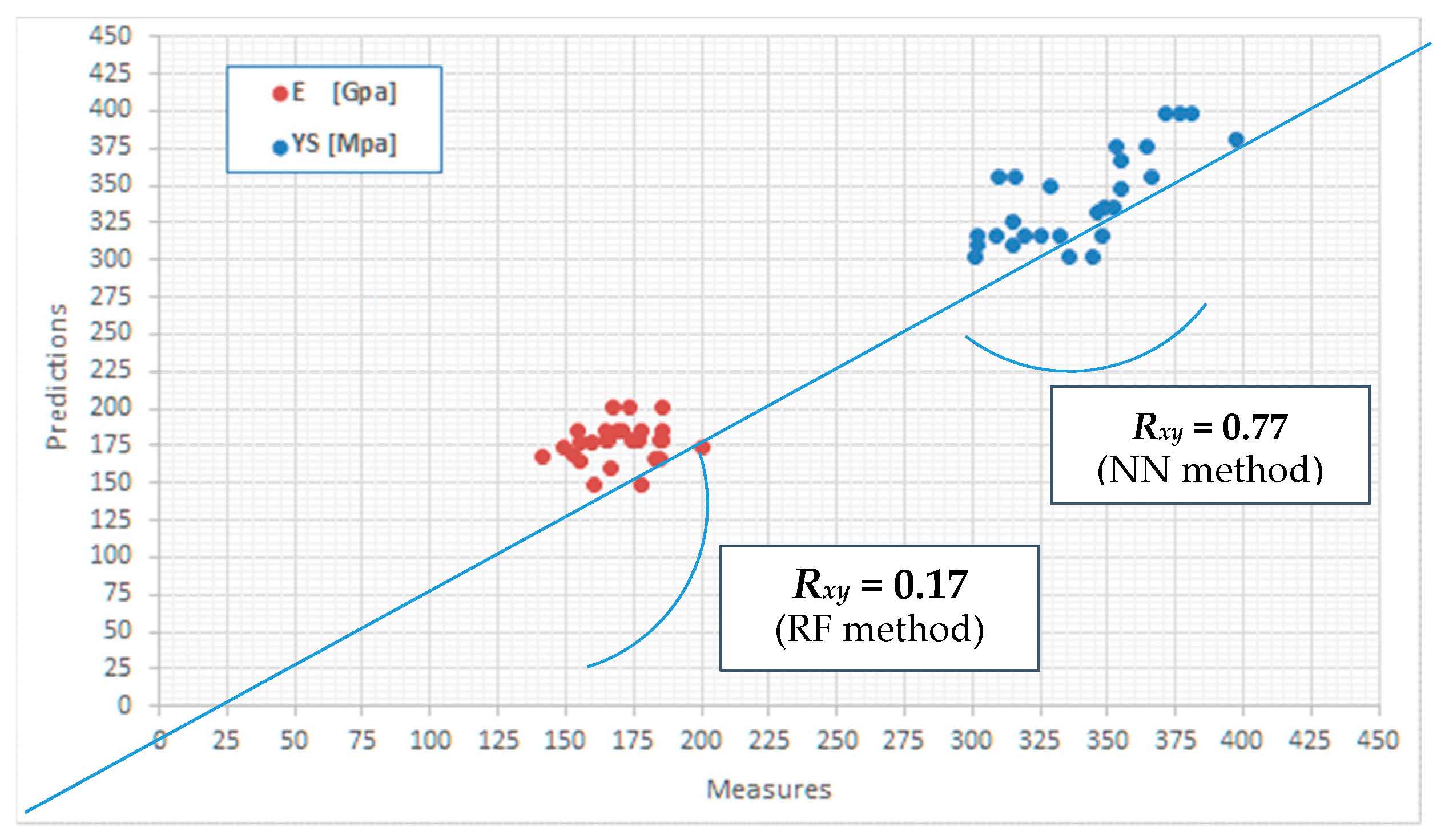
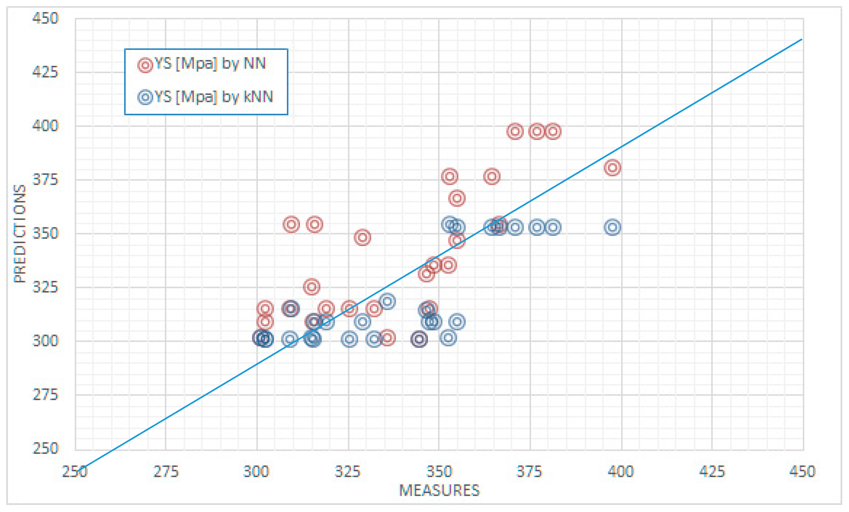
Young’s modulus (E)	4.1%	0.0%	−7.6%	2.7%	−2.7%	−9.3%

, the distance between the measured and predicted values are reported in terms of percentage errors with respect to the average values of tensile properties. It is evident how, except in rare cases, all the different algorithms can provide valid predictions. Also, in the present case, the confidence placed by Reference [59] in the possibility of accelerating material property predictions by the use of machine learning is confirmed.

In particular, of 24 values under investigation, 7 of them (almost 1/3) are predicted with an error lower than 1%; 11 lower than 3%; 16 (equal to 2/3) lower than 6%. In addition, it can also be noted that the uncorrected values (with percentage errors > 10%) are essentially related to the prediction of the Ultimate Strain (ε).

Even in this extreme case, the correspondence is quite acceptable, as demonstrated in Figure 3 where the comparison between measures and predictions is shown in terms of values frequency. It is possible to see how the density functions for measures and predictions overlap in several situations as, for example, in the cases of RF and NN methods for the Ultimate Strain (ε). Actually, it is possible to say that the NN method can closely retrace the density functions for all the situations under investigation. It means, in practice, that the NN method can predict the real values not limited to the average values but also through its range of variability. This good accuracy in predicting the mechanical properties of cast iron offered by the NN method was also reported by Reference [61] with respect to an investigation involving 24 process parameters and 800 external data.

It is not the case that the kNN method shows a tendency to systematically underestimate reality (shown by narrow curves, shifted on the left, towards lower average values). These graphs are related to SGI but similar considerations emerge from data analysis in the case of CGI.

It is also worth noting that the validity of the predictions by ML does not seem to be affected by the specific values assumed by the properties. This contrasts with Reference [28], where it was reported that the prediction by the expert system ceased to be accurate for UTS higher than 100 MPa—in this analysis, the estimation methods proved to be equally valid for two cast iron families with very different properties, that is, SGI and CGI with an UTS of, respectively, 539 and 337 MPa.

Furthermore, it is confirmed that the potentiality of CGI in replacing SGI in particular applications where ductivity may be preferred to high stiffness, as expressed by References [4,62,63].

5.6. Correlations

Even if a prediction is accurate with respect to the average values and to the variability of measures, their distribution could be significantly different. Thus, the linear correlation is also investigated. In

Table 8. Correlation between measures and predictions in terms of Pearson correlation coefficient.

Pearson Correlation Coefficient (rxy)	SGI			CGI
	RF	NN	k-NN	RF	NN	kNN
Ultimate Tensile Strength (UTS)	0.39	0.76	0.81	0.48	0.41	0.37
Yield Strength (YS)	0.56	0.74	0.79	0.33	0.33	0.22
Ultimate Strain (ε)	−0.12	0.17	−0.14	0.29	0.50	0.19
Young’s modulus (E)	0.17	−0.07	−0.05	−0.02	−0.48	−0.41

, the linear relations between measured and predicted values are reported in terms of Pearson correlation coefficients: as mentioned, the correlation is much better than the value closer to 1.

Figure 4 reports a graphical representation of the meaning of this linear correlation proposing a comparison between data with difference Pearson correlation coefficients (r_xy). It is the case, in particular, of the values of Yield Strength (YS) and the Young’s modulus (E) for SGI, characterized by Pearson correlation coefficients of 0.74 (predicted by NN) and 0.17 (predicted by RF), respectively. The same diagram shows, simultaneously, properties with different units—namely (MPa) and (GPa)—and each point represents a single prediction, positioned by the experimental (x-axis) and predicted (y-axis) values. In this chart, points that are distributed along the bisector (x = y) or very close to it—as the values of Yield Strength (YS)—demonstrate a good correlation between experimental measurements and numerical predictions. On the contrary, a distribution of points like clouds, as in the case of Young’s modulus (E) values, demonstrates a lack of correlation between measures and prediction.

Instead, Figure 5 reports a graphical representation of data characterized by (substantially) equal Pearson correlation coefficients.

It is the case, for instance, of the values of Yield Strength (YS) for SGI where those coefficients are 0.74 or 0.76, depending on the specific ML methods used (NN and kNN, respectively). The correspondence between the coefficients suggests that the two forecasting techniques are similarly effective. At the same time, the diagram shows how some aspects can escape attention if the analysis remains limited to the coefficients. In the figure, it is observed, for instance, how the values predicted by kNN are not randomly distributed around the bisector but are all shifted to the right. This means, in practice, that the kNN method proposes predictions subject to a slight, but systematic, error of underestimation, confirming the similar considerations on the kNN method previously emerged.

5.7. Results Summary

In brief, the accuracy of ML methods in predicting the mechanical properties starting from the metallurgical properties, as estimated by images analysis samples and macro-indicators, was evaluated comparing measures and predictions with respect to their mean values (μ)/standard deviations (σ) (Table 7) and by the overall trend of the Pearson coefficients (r_xy) (Table 8). The comparison is also shown by representing, respectively, the way the density functions, defined by μ and σ, overlap (Figure 3) and how these values are distributed, point to point, in correlation graphs (Figure 4 and Figure 5).

Thanks to this analysis it is possible to propose, as results, the following considerations:

-

ML methods confirm their general validity in predicting the mechanical properties of metals;

-

this seems true, even in the presence of a quite limited dataset to be used for training;

-

information can be directly taken from micrographs by a conventional process of image analysis and macro-indicators without the need to go through deeper metallurgical investigations;

-

in particular, the NN method seems the most appropriate of those considered;

-

the kNN method, although it has good accuracy, also shows a tendency to systematic errors;

-

the accuracy in prediction is different for each specific property under investigation, achieving the best results for UTS and YS but also offering acceptable indications in the other cases;

-

the average values of experiments and predictions (measured by μ) often coincide in practice;

-

the deviation with respect to the average values (measured by σ) shows a variability in prediction in line with the intrinsic variability as revealed by the experimental measurements;

-

the Pearson correlation (r_xy) can be conveniently adopted for a quick evaluation of data but also for the validation of predictions.

6. Conclusions

There is no doubt that Artificial Intelligence (AI) and Machine Learning (ML) have become widely known over the past few years thanks to their applicability. As Big Data technologies retain the status of the most discussed IT trend of modernity, so ML algorithms can be considered the most powerful tool focused on the predictive application of large amounts of data. It is the same in the material sciences.

This article proposed the use of three between the most common ML algorithms, available in an open source platform, in supporting the material data analysis. In particular, the Random Forest, the Artificial Neural Network and the k-nearest neighbours methods have been preferred for pattern recognition on two datasets of tensile properties of two different foundry alloys—ductile and compact graphite cast irons—as measured in previous experiments. The Expert System, trained on these (extremely limited number of) data, provided predictions in line with the measures, both in terms of mean values and variability, in large part of the situations under investigation. In particular, an extremely accurate correspondence between experimental and predicted data along the full range of values emerges in the case of Ultimate Tensile Strength (UTS) and Yield Strength (YS), with errors lower than 1% (when considered in terms of mean/expected values). But even in the other situations under examination, related to the Ultimate Strain (ε) and Young’s modulus (E), the use of AI as an investigation system could provide valid support. As a consequence, it is possible to confirm the benefit of the ML techniques in predicting the mechanical properties of cast alloys. Furthermore, they could help with investigating the strict relationship between these ultimate properties and other fundamental aspects of metallurgy, as constituent elements, microstructures, process parameters or treatments.

Finally, it is worth considering how the validity in prediction could be reasonably improved: selecting additional Machine Learning classifiers, optimizing their parameters and enlarging the dataset adopted for training. All these improvements in the investigation approach are relatively simple without introducing any additional complexity to the predicting procedure.

References

1. Ashby, M.F.; Jones, D.R.H. Engineering Materials 1: An Introduction to Properties, Applications and Design, 4th ed.; Elsevier: Oxford, UK, 2012. [Google Scholar]
2. Hans, E.; Koski, J.; Osyczka, A. Multicriteria Design Optimization: Procedures and Applications; Springer Science & Business Media: Berlin, Germany, 2012. [Google Scholar]
3. Boyles, A. The Structure of Cast Iron: A Series of Three Educational Lectures on the Structure of Cast Iron; American Society for Metals: Russell Township, OH, USA, 1947. [Google Scholar]
4. Fragassa, C. Material selection in machine design: The change of cast iron for improving the high-quality in woodworking. Proc. Inst. Mech. Eng. C J. Mech. Eng. Sci. 2016, 231, 18–30. [Google Scholar] [CrossRef]
5. Campbell, F.C. Elements of Metallurgy and Engineering Alloys; ASM International: Materials Park, OH, USA, 2008; p. 453. [Google Scholar]
6. Elliott, R. Cast Iron Technology; Butterworth-Heinemann: London, UK, 1988. [Google Scholar]
7. Sinha, A.K. Physical Metallurgy Handbook; McGraw-Hill Professional Publishing: New York, NY, USA, 2003. [Google Scholar]
8. Damir, A.N.; Elkhatib, A.; Nassef, G. Prediction of fatigue life using modal analysis for grey and ductile cast iron. Int. J. Fatigue 2007, 29, 499–507. [Google Scholar] [CrossRef]
9. Elkholy, A. Prediction of abrasion wear for slurry pump materials. Wear 1983, 84, 39–49. [Google Scholar] [CrossRef]
10. Berdin, C.; Dong, M.J.; Prioul, C. Local approach of damage and fracture toughness for nodular cast iron. Eng. Fract. Mech. 2001, 68, 1107–1117. [Google Scholar] [CrossRef]
11. Kim, J.; Bae, C.; Woo, H.; Kim, J.; Hong, S. Assessment of residual tensile strength on cast iron pipes. In Pipelines 2007: Advances and Experiences with Trenchless Pipeline Projects; Mohammad Najafi, P.E., Lynn Osborn, P.E., Eds.; ASCE: Reston, VA, USA, 2007; pp. 1–7. [Google Scholar]
12. Atkinson, K.; Whiter, J.T.; Smith, P.A.; Mulheron, M. Failure of small diameter cast iron pipes. Urban Water 2002, 4, 263–271. [Google Scholar] [CrossRef]
13. Fragassa, C.; Zigulic, R.; Pavlovic, A. Push-pull fatigue test on ductile and vermicular cast irons. Eng. Rev. 2016, 36, 269–280. [Google Scholar]
14. Álvarez, L.; Luis, C.J.; Puertas, I. Analysis of the influence of chemical composition on the mechanical and metallurgical properties of engine cylinder blocks in grey cast iron. J. Mater. Process. Technol. 2004, 153, 1039–1044. [Google Scholar] [CrossRef]
15. Fragassa, C.; Minak, G.; Pavlovic, A. Tribological aspects of cast iron investigated via fracture toughness. Tribol. Ind. 2016, 38, 1–10. [Google Scholar]
16. Li, Y.; Chen, W.; Huang, D.; Luo, J.; Liu, J.; Chen, Y.; Liu, Q.; Su, S. Energy conservation and emissions reduction strategies in foundry industry. China Foundry 2010, 7, 392–399. [Google Scholar]
17. Gonzaga, R.A.; Carrasquilla, J.F. Influence of an appropriate balance of the alloying elements on microstructure and on mechanical properties of nodular cast iron. J. Mater. Process. Technol. 2005, 162, 293–297. [Google Scholar] [CrossRef]
18. McNeil, I. An Encyclopedia of the History of Technology; Routledge: London, UK, 2002. [Google Scholar]
19. Angus, H.T. Cast Iron: Physical and Engineering Properties; Elsevier: London, UK, 2013. [Google Scholar]
20. Collini, L.; Nicoletto, G.; Konečná, R. Microstructure and mechanical properties of pearlitic gray cast iron. Mater. Sci. Eng. A 2008, 488, 529–539. [Google Scholar] [CrossRef]
21. Radovic, N.; Morri, A.; Fragassa, C. A study on the tensile behaviour of spheroidal and compacted graphite cast irons based on microstructural analysis. In Proceedings of the 11th IMEKO TC15 Youth Symposium on Experimental Solid Mechanics, Brasov, Romania, 30 May–02 June 2012; pp. 185–190. [Google Scholar]
22. Fragassa, C.; Pavlovic, A. Compacted and spheroidal graphite irons: Experimental evaluation of Poisson’s ratio. FME Trans. 2016, 44, 327–332. [Google Scholar] [CrossRef]
23. Fragassa, C.; Radovic, N.; Pavlovic, A.; Minak, G. Comparison of mechanical properties in compacted and spheroidal graphite irons. Tribol. Ind. 2016, 38, 49–59. [Google Scholar]
24. Tiedje, N. Solidification, processing and properties of ductile cast iron. Mater. Sci. Technol. 2010, 26, 505–514. [Google Scholar] [CrossRef]
25. Costa, N.; Machado, N.; Silva, F.S. A new method for prediction of nodular cast iron fatigue limit. Int. J. Fatigue 2010, 32, 988–995. [Google Scholar] [CrossRef]
26. Shiraki, N.; Usui, Y.; Kanno, T. Effects of number of graphite nodules on fatigue limit and fracture origins in heavy section spheroidal graphite cast iron. Mater. Trans. 2016, 57, 379–384. [Google Scholar] [CrossRef]
27. Santos, C.A.; Spim, J.A., Jr.; Ierardi, M.C.; Garcia, A. The use of artificial intelligence technique for the optimisation of process parameters used in the continuous casting of steel. Appl. Math. Modell. 2002, 26, 1077–1092. [Google Scholar] [CrossRef]
28. Calcaterra, S.; Campana, G.; Tomesani, L. Prediction of mechanical properties in spheroidal cast iron by neural networks. J. Mater. Process. Technol. 2000, 104, 74–80. [Google Scholar] [CrossRef]
29. Roshan, H.D.; Sudesh, K. Expert system for analysis of casting defects: Cause module. Trans. Am. Foundrymen’s Soc. 1989, 97, 601–606. [Google Scholar]
30. Artificial Intelligence. Available online: https://en.wikipedia.org/wiki/Artificial_intelligence (accessed on 15 March 2019).
31. Fukunaga, K. Introduction to Statistical Pattern Recognition; Elsevier: Amsterdam, The Netherlands, 2013. [Google Scholar]
32. Dong, M.J.; Hu, G.K.; Diboine, A.; Moulin, D.; Prioul, C. Damage modelling in nodular cast iron. J. Phys. IV 1993, 3, 643–648. [Google Scholar] [CrossRef]
33. Gonzaga, R.A. Influence of ferrite and pearlite content on mechanical properties of ductile cast irons. Mater. Sci. Eng. A 2013, 567, 1–8. [Google Scholar] [CrossRef]
34. Radisa, R.; Ducic, N.; Manasijevic, S.; Markovic, N.; Cojbasic, Z. Casting improvement based on metaheuristic optimization and numerical simulation. Facta Univ. Ser. Mech. Eng. 2017, 15, 397–411. [Google Scholar] [CrossRef]
35. Voracek, J. Prediction of mechanical properties of cast irons. Appl. Soft Comput. 2001, 1, 119–125. [Google Scholar] [CrossRef]
36. Kohavi, R.; Provost, F. Glossary of terms. Mach. Learn. 1998, 30, 271–274. [Google Scholar]
37. Weiss, S.M.; Kulikowski, C.A. Computer Systems That Learn: Classification and Prediction Methods from Statistics, Neural Nets, Machine Learning and Expert Systems; Morgan Kaufmann: San Mateo, CA, USA, 1991; Volume 123. [Google Scholar]
38. Bishop, C.M. Pattern Recognition and Machine Learning; Springer: New York, NY, USA, 2006. [Google Scholar]
39. Anzai, Y. Pattern Recognition and Machine Learning; Elsevier: Amsterdam, The Netherlands, 2012. [Google Scholar]
40. Maulik, U.; Sanghamitra, B. Genetic algorithm-based clustering technique. Pattern Recognit. 2000, 33, 1455–1465. [Google Scholar] [CrossRef] [Green Version]
41. Samuel, A.L. Some studies in machine learning using the game of checkers. IBM J. Res. Dev. 2000, 44, 206–226. [Google Scholar] [CrossRef] [Green Version]
42. Schmidhuber, J. Deep learning in neural networks: An overview. Neural Netw. 2015, 61, 85–117. [Google Scholar] [CrossRef] [Green Version]
43. Hughes, I.C.H.; Powell, J.; de Albuquerque, V.H.C.; Cortez, P.C.; de Alexandria, A.R.; Tavares, J.M.R. A new solution for automatic microstructures analysis from images based on a backpropagation artificial neural network. Nondestr. Test. Eval. 2008, 23, 273–283. [Google Scholar] [Green Version]
44. Perzyk, M.; Kochański, A.W. Prediction of ductile cast iron quality by artificial neural networks. J. Mater. Process. Technol. 2001, 109, 305–307. [Google Scholar] [CrossRef]
45. Ward, L.; Agrawal, A.; Choudhary, A.; Wolverton, A. A general-purpose machine learning framework for predicting properties of inorganic materials. Comput. Mater. 2016, 2, 16028. [Google Scholar] [CrossRef] [Green Version]
46. Liu, Y.; Zhao, T.; Ju, W.; Shi, S. Materials discovery and design using machine learning. J. Materiomics 2017, 3, 159–177. [Google Scholar] [CrossRef]
47. SCM Foundry. Available online: http://www.scmfonderie.it/?l=en&p=azienda (accessed on 15 November 2015).
48. Altstetter, J.D.; Nowicki, R.M. Compacted Graphite Iron—Its properties and automotive applications. AFS Trans. 1982, 82, 959–970. [Google Scholar]
49. BS EN ISO 1563. Founding. Spheroidal Graphite Cast Iron; BSI: London, UK, 2012. [Google Scholar]
50. EN ISO 6892-1. Metallic Materials—Tensile Testing—Part 1: Method of Test at Room Temperature; ISO: Geneva, Switzerland, 2016. [Google Scholar]
51. Orange Platform. Available online: https://orange.biolab.si/ (accessed on 10 April 2019).
52. Wolpert, D.H.; Macready, W.G. No free lunch theorems for optimization. IEEE Trans. Evol. Comput. 1997, 1, 67. [Google Scholar] [CrossRef]
53. Wolpert, D. The lack of a priori distinctions between learning algorithms. Neural Comput. 1996, 8, 1341–1390. [Google Scholar] [CrossRef]
54. Babic, M.; Calì, M.; Nazarenko, I.; Fragassa, C.; Ekinovic, S.; Mihaliková, M.; Janjić, M.; Belič, I. Surface roughness evaluation in hardened materials by pattern recognition using network theory. Int. J. Interact. Des. Manuf. 2018, 13, 211–219. [Google Scholar] [CrossRef]
55. Lin, Y.; Yongho, J. Random forests and adaptive nearest neighbours. J. Am. Stat. Assoc. 2006, 101, 578–590. [Google Scholar] [CrossRef]
56. Gurney, K. An Introduction to Neural Networks; CRC Press: London, UK, 2014. [Google Scholar]
57. Garcia, S.; Derrac, J.; Cano, J.; Herrera, F. Prototype selection for nearest neighbour classification: Taxonomy and empirical study. IEEE Trans. Pattern Anal. Mach. Intell. 2012, 34, 417–435. [Google Scholar] [CrossRef] [PubMed]
58. Wagner, N.; Rondinelli, J.M. Theory-guided machine learning in materials science. Front. Mater. 2016, 3, 28. [Google Scholar] [CrossRef]
59. Pilania, G.; Wang, C.; Jiang, X.; Rajasekaran, S.; Ramprasad, R. Accelerating materials property predictions using machine learning. Sci. Rep. 2013, 3, 2810. [Google Scholar] [CrossRef] [PubMed]
60. Zhang, Y.; Ling, C. A strategy to apply machine learning to small datasets in materials science. Npj Comput. Mater. 2018, 4, 25. [Google Scholar] [CrossRef]
61. Sata, A. Mechanical property prediction of investment castings using artificial neural network and multivariate regression analysis. In Proceeding of the 63rd Indian Foundry Congress, Greater Noida, India, 27 February–1 March 2015. [Google Scholar]
62. Lucisano, G.; Stefanovic, M.; Fragassa, C. Advanced design solutions for high-precision woodworking machines. Inter. J. Qual. Res. 2016, 10, 143–158. [Google Scholar]
63. Dawson, S.; Schroeder, T. Practical applications for compacted graphite iron. AFS Trans. 2004, 47, 1–9. [Google Scholar]
Figure 1. Metallurgical properties ((a) Ultimate Tensile Strength (UTS), (b) Yield Strength (YS), (c) Ultimate Strain (ε), (d) Young’s modulus (E)) in the case of Spheroidal Graphite Iron (SGI), as measured and predicted.
Metals 09 00557 g001aMetals 09 00557 g001b
Figure 2. Metallurgical properties ((a) Ultimate Tensile Strength (UTS), (b) Yield Strength (YS), (c) Ultimate Strain (ε), (d) Young’s modulus (E)) in the case of Compacted Graphite Iron (CGI), as measured and predicted.
Metals 09 00557 g002aMetals 09 00557 g002b
Figure 3. Comparison between measured and predicted values in terms of density functions (case of SGI) for: (a) Ultimate Tensile Stress; (b) Yield Stress; (c) Ultimate Strain; (d) Young’s Modulus.
Metals 09 00557 g003
Figure 4. A graphical representation of data with different Pearson correlation coefficients. It is the case of YS (MPa) and E (GPa) for SGI with coefficients of, respectively, 0.74 (NN) and 0.17 (RF).
Metals 09 00557 g004
Figure 5. A graphical representation of data with equal Pearson correlation coefficients. It is the case of YS (MPa) for SGI with coefficients of, respectively, 0.74 (NN) and 0.79 (kNN).
Metals 09 00557 g005