Mathematical Modeling of Postcombustion in an Electric Arc Furnace (EAF)

Abstract

Numerical modeling was used to study the capability of postcombustion in an electric arc furnace (EAF) equipped with virtual lance burners. The CO flow rate at the molten bath surface was estimated using the off-gas data obtained close to the outlet of an EAF. Then, the effect of the secondary oxygen flow rate on postcombustion was studied. The results show a CO flow rate of 0.6 kg·s⁻¹ and 0.8 kg·s⁻¹ for operation modes of burner and burner + lancing. Increase of the secondary oxygen flow rates of 60% and 70% result in 17% and 7% increase in the postcombustion ratio (PCR) for the burner and burner lancing modes, respectively.

1. Introduction

The high amount of carbon monoxide produced in an electric arc furnace (EAF) is an important source of chemical energy. The heat generated by postcombustion (PC) of CO can be captured by scrap. This contributes to a reduction of the electrical energy in an EAF. The PC process can be applied effectively in EAFs by using PC systems designed as supersonic oxygen injectors embedded in the furnace walls [1,2,3,4,5]. The supersonic jets result in an increased gas penetration into the melt compared to the subsonic ones which is caused by a high dynamic pressure. However, superstoichiometric ratios of oxygen to fuel in burners can also improve the PC efficiency [5].

Li and Fruehan [2] used computational fluid dynamics (CFD) to study the effect of PC on the heat generation in an EAF equipped with four PC injectors. The de-PC reaction, due to the reaction of CO₂ with carbon in the melt and the electrode surfaces, was included in the model. Their results showed that the heat transfer efficiency is lower for a flat bath condition than for a bath containing a scrap pile. Besides, de-PC reduces the amount of CO₂ and as a result, less chemical energy is available in the furnace. Januard et al. [3] studied PC optimization in an industrial furnace equipped with a PC injector tool. They used a dynamic control and set points to control the oxygen injectors. The amount of CO and CO₂ was monitored continuously using near infrared (IR) laser diode spectroscopy during the furnace operation. A high concentration of CO₂ was observed during the refining stage during the foaming slag formation. Zhonghua et al. [4] also developed a CFD model to study PC in an EAF. The reaction rate was determined based on both temperature and turbulence data. They showed that when using multiple top PC injectors and oxygen, an excess ratio can improve the PC efficiency.

Thomson et al. [5] studied the effect of the burner oxygen to fuel ratio on the energy efficiency of an EAF using the data from off-gas determinations. The electrical energy consumption and tap-to-tap time was reduced due to a higher burner oxygen to fuel ratio.

Chan et al. [6] focused on the formation of NOx due to the air ingress from the slag door using a CFD model. Reduced CO and H₂ levels due to a generation of NO were observed. They also showed that an additional oxygen injection through the burners increases the furnace temperature representative for PC reactions.

The EAF modelled in this study represents an existing furnace equipped with a virtual lance burner (VLB) system. The VLB system is a compact injection tool which operates in the three main modes of (i) burner, (ii) burner + lancing, and (iii) lancing. It consists of three inlets to supply the main oxygen, secondary oxygen, and fuel. Melting of scrap and heating up the cold zones inside the furnace starts in the burner mode, and refining starts in the burner + lancing mode by increasing the flow rate of oxygen from the main nozzle. Previous studies showed that the power-on time and electrical energy is reduced in EAFs using VLB systems [7,8]. Figure 1a shows the geometry of the fluid inside the modelled VLB. The inlets and outlets for oxygen and fuel are shown at the left and right sides of the figure, respectively.

A summary of previous CFD models studying combustion in EAF is shown in

Table 1. Summary of previous computational fluid dynamics (CFD) models.

Ref., Date	CFD Model	Dim	Reactions	Predictions	Combustion Source	Off-Gas Data	Domain
Li et al., 2003 [3]	Chemical-reaction Species Radiation	3D	PC of CO Dissociation of CO2 de-PC	Temperature profile Mass transfer of CO, O2 and CO2 Radiation	Oxygen injectors	Y	Whole furnace
Chan et al., 2004 [6]	Species * Radiation	3D	Combustion of CO, H2, and CH4 and NO formation	Temperature profile Mass transfer of NO, CO and O2	Burner Oxygen lancing	Y	Whole furnace
Zhonghua et al., 2009 [4]	Species * Radiation	3D	Combustion of CO	Mass transfer of CO and O2	Oxygen injectors	N	Whole furnace
Current work	Species * Radiation	3D	Combustion of CO, H2 and CH4	Temperature profile Mass transfer of CO, O2 and CO2	Secondary oxygen of the burner	Y	Whole furnace

* Eddy dissipation model (EDM) for turbulent mixing and finite rate mode (FRM) for chemical kinetics.

. In these CFD models, the combustion source was oxygen injectors installed for the PC, while in this study, a CFD model is developed to study the influence of the VLB efficiency on the PC in an EAF. This is done by adjusting the secondary oxygen flow rate to increase PC.

2. Model Description

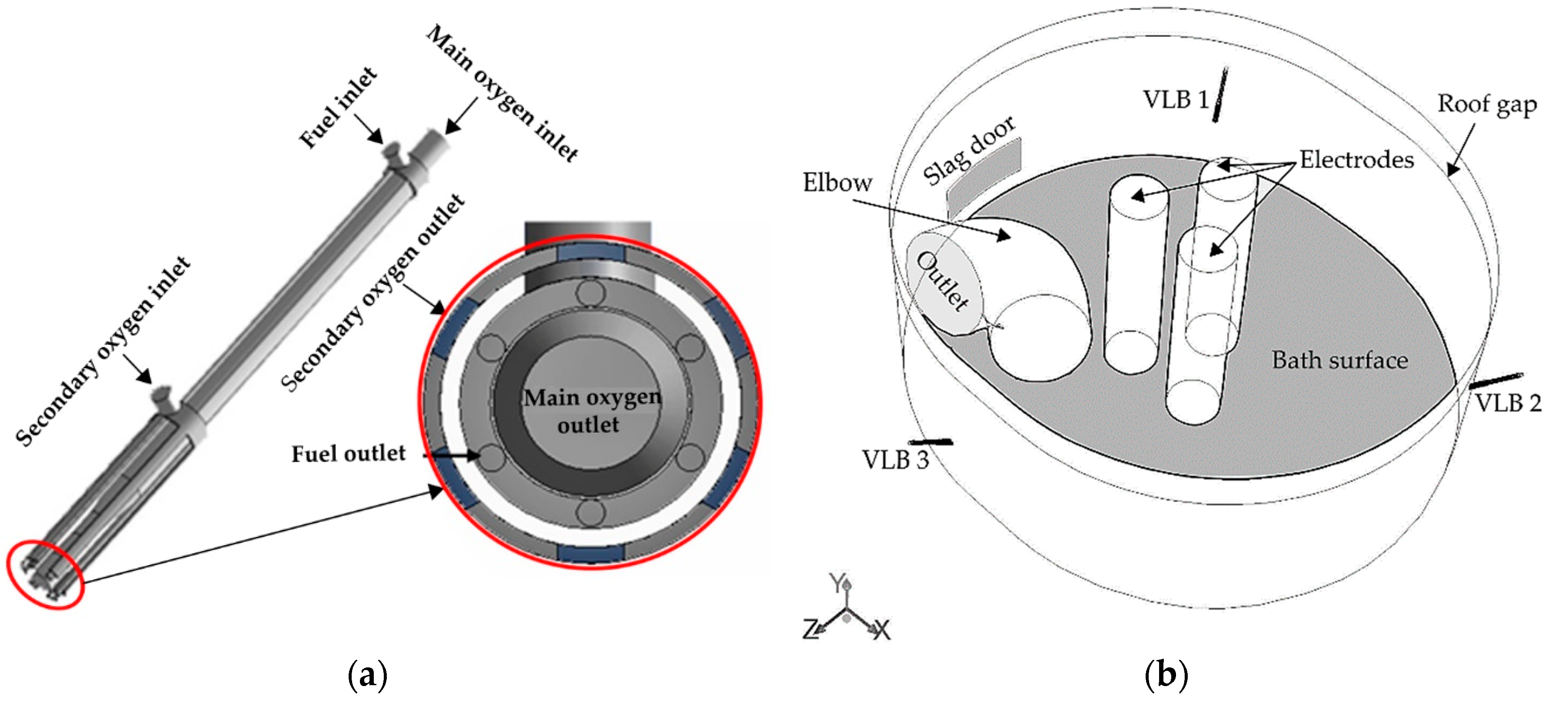
2.1. Computational Domain

The computational domain is the gas phase above the molten bath surface around the electrodes, the fluid inside three VLBs located at the furnace wall and the elbow (Figure 1b). The enlarged domain of the fluid inside the VLB is shown in Figure 1b. The main oxygen is injected into the furnace through the central nozzle, and six secondary oxygen and six fuel jets are located around the main oxygen nozzle.

The main assumptions applied to simplify the model were as follows:

• A flat molten bath surface
• A constant flow rate of CO from the molten bath surface
• No generation of NOx inside the furnace

2.2. Reactions and Governing Equations

A steady-state gas flow was modeled by solving the mass, momentum, energy, and species conservation equations.

The simplified form of oxy-fuel reaction [9] overpredicts the temperature and concentration of species, but it was applied for simplicity as:

CH₄ + 2O₂ → CO₂ + 2H₂O

(1)

Combustion of CO was assumed to be irreversible:

CO + 0.5O₂ → CO₂

(2)

Dissociation reactions for species such as oxygen, water, and carbon dioxide were not taken into account. However, in order to avoid an overestimation of the temperature, a modified heat-specific capacity for each species was applied.

The species source term in the species conservation equation was determined using the kinetic rate (R_k) and turbulence mixing rate (R_e) which are described below. Both were computed, and the lower value was used as the limiting rate of the reaction.

The molar kinetic rate of reaction was calculated as [10]:

$$R_{j,k}=\left(v_{j,r}^{″}- v_{j,r}^{″}\right)k_{f,r}{\displaystyle \prod }_{j=1}^{N_R}{C}_{j,r}{\eta }_{j,r}^{\prime }+{\eta }_{j,r}^{″}$$

(3)

where $C_{j,r}$ is the molar concentration of species j in reaction r, ${\eta }_{j,r}^{\prime }$ is the exponent rate for reactant species j in reaction r, N_R is the number of reactions, ${\eta }_{j,r}^{″}$ is the exponent rate for product species j in reaction r, $v_{j,r}^{″}$ is the stoichiometric coefficient of products, $v_{j,r}^{\prime }$ is the stoichiometric coefficient of reactants, and $k_{f,r}$ is the forward rate constant. It is a function of temperature according to the Arrhenius expression which is defined as [10]:

$$k_{f,r}=A_r{T}^{\beta }\exp \left(-\frac{E_r}{RT}\right)$$

(4)

where β is the temperature exponent, $A_r$ is the pre-exponential factor, and $E_r$ is the activation energy for the reaction, presented for all reactions in

Table 2. Constants used in the calculations of the kinetic reaction rate for Reactions 1 and 2 [11].

Reaction	(1)	(2)
$A_r$	2.119 $\times {10}^{11}$	2.239 $\times {10}^{12}$
E (J/kmol)	2.027 $\times {10}^8$	1.7 $\times {10}^8$
β	0	0
${\eta }_{O2}^{\prime }$	1.3	0.25
${\eta }_{CO}^{\prime }$	-	1
${\eta }_{H2O}^{″}$	-	0.5
${\eta }_{CH4}^{\prime }$	0.2	-
${\eta }_{H2}^{\prime }$	-	-
${\eta }_{CO2}^{\prime }$	-	-

[11].

The turbulence rate was calculated using the two following expressions for the rate of combustion. The lower value determines the rate of reaction.

$$R_{j,e}=v_j^{\prime }A{M}_{w,j}\rho \frac{\epsilon }{k}\underset{R}{\min }\left(\frac{Y_R}{v_R^{\prime }{M}_{w,R}}\right)$$

(5)

$$R_{j,e}= v_j^{\prime }{M}_{w,j}AB\frac{\epsilon }{k}\frac{{\sum }_P{Y}_P}{{\sum }_j^N{v}_j^{″}{M}_{w,j}}$$

(6)

where $Y_R$ and $Y_P$ are the mass fractions of product species P and reactant species R, respectively. Furthermore, k is the kinetic turbulence kinetic energy, $\epsilon$ is the turbulence dissipation rate, N is the number of species, and $M_{w,j}$ is the molecular weight of species j. A is a constant for reactants equal to 4 and B is the product constant equal to 0.5 [12].

2.3. Material Properties

As mentioned earlier, to avoid an overprediction of temperature, the heat-specific capacity for each species was modified as a polynomial function of the temperature using the data applied by Peters and Weber [13].

The density of the gas was calculated from the ideal gas law:

$$\rho =\frac{P}{\frac{R}{M_w}T}$$

(7)

where P is the absolute pressure, and R is the gas constant.

2.4. Boundary Conditions

The boundary conditions were acquired from actual plant data as well as data from literature studies.

• Bottom: CO arises from the bottom surface of the domain. The flow rate of CO is mainly dependent on the decarburization rate and carbon-injection amount. A flow rate of 0.5 kg·s⁻¹ from the molten bath for the burner mode (decarburization rate of 0.04% C min⁻¹) and a flow rate of 1 kg·s⁻¹ from the molten bath for the burner and lancing mode (decarburization rate of 0.08% C min⁻¹) are assumed. It should be mentioned that these values are very dependent on the oxygen efficiency (the maximal possibility that the carbon in the melt reacts with the oxygen) which is difficult to measure. Temperature at the bottom surface is assigned to steel melting temperature 1773 K.
• VLB: Oxygen and methane gas are injected from three VLBs mounted at the wall at an angle of 40° to the molten bath surface.

According to the off-gas measurements, the concentration of CO starts to increase at the burner + lancing (B+L) mode. However, both the final burner mode (B3) and B+L1 modes are considered since there is still an amount of scrap inside the furnace. Therefore, the optimum PC can be achieved in these periods, and the generated energy can return to the charged materials.

Oxygen injected from the main nozzle mainly reacts with the carbon in the melt during decarburization as well as with injected carbon during the slag foaming period. Overall, only a small amount of the main oxygen can contribute to postcombustion.

Two methods are used to prevent the oxygen from the main nozzle to react with CO from the bath. In the first method, a part of the oxygen (90% in mole fraction) is excluded from the reaction, but it is not removed from the furnace. In the second method, oxygen is removed from the furnace close to the bottom of the domain, at a height of 0.05 m. This means that the oxygen is removed from all cells adjacent to the bath surface. A sink source (in kg·m⁻³·s⁻¹) is added in the mass conservation equation for oxygen. This source term is defined as $-M_{O_2}\left(\frac{\partial C_{O_2}}{\partial t}\right)$ due to the decarburization reaction (C_melt + 0.5O_2(g) → CO_(g)), where $M_{O_2}$ is the molar mass of oxygen, and $\frac{\partial C_{O_2}}{\partial t}$ is the chemical rate of consumption of oxygen (mol·m⁻³·s⁻¹). The oxidization of other elements in the melt (such as Fe, Si, Mn, etc.) was neglected.

The boundary conditions applied to three inlets to supply the main oxygen, secondary oxygen, and fuel were taken from the studied EAF, shown in

Table 3. Oxygen and methane mass flow rates in VLB modes for melting and melting + refining.

Stage	Mode	Main Oxygen (kg·s−1)	Secondary Oxygen (kg·s−1)	Methane (kg·s−1)
Melting	Burner (B1)	0.119	0.099	0.052
	Burner (B2)	0.063	0.198	0.064
	Burner (B3)	0.198	0.063	0.064
Melting + Refining	Burner + Lancing (B+L1)	0.317	0.059	0.052
	Burner + Lancing (B+L2)	0.396	0.059	0.043
Refining	Lancing (L)	0.634	0.04	0.023

. Note that plug flow was assumed for all inlets.

The fuel is injected through the fuel inlet, so the equivalent mass flow rate is used for methane. The temperature of both oxygen and methane is 298 K.

• VLB walls: A constant temperature of 300 K is assigned to the VLB walls. No-slip and standard wall function.
• Slag door: For one of the cases, the air infiltration through the slag door was considered. The mass flow rate and temperature are assigned to values of 0.1 kg·s⁻¹ and 800 K. In the other cases, the slag door was considered as a wall.
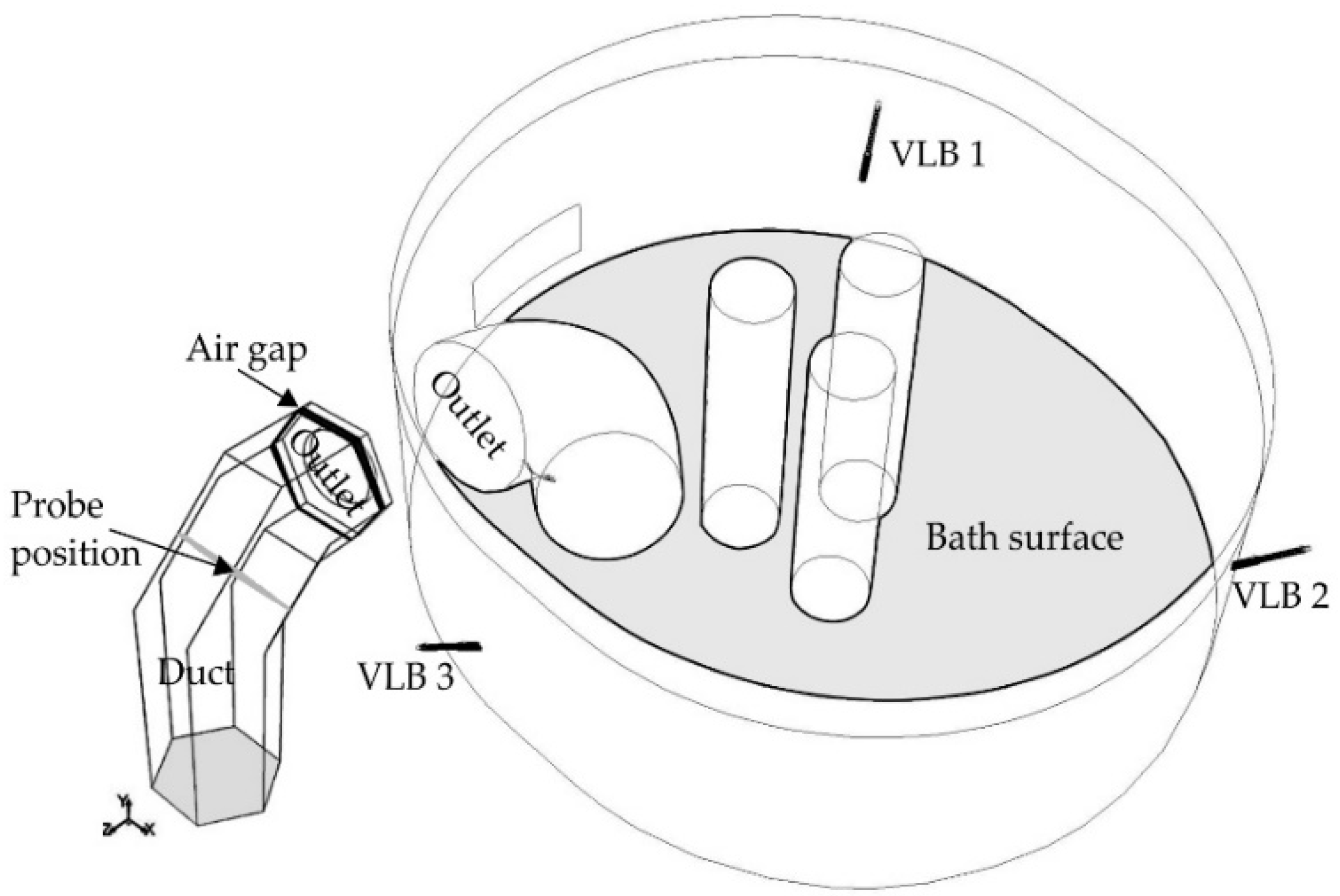
• Outlet: Pressure outlet where the off-gas chemical composition data from other EAFs are used for the backflow volume fractions of species. Temperature was specified from EAF data and low values for k and ε are applied as backflow condition.
• Electrodes: Zero heat flux is assumed on surfaces of the electrodes.
• Roof, side walls, and duct walls: A constant temperature of 1000 K is assigned to the side walls duct walls and roof. No-slip and standard wall function.
• Roof ring gap: The air ingresses through the roof ring gap which is specified as a mass flow rate inlet.

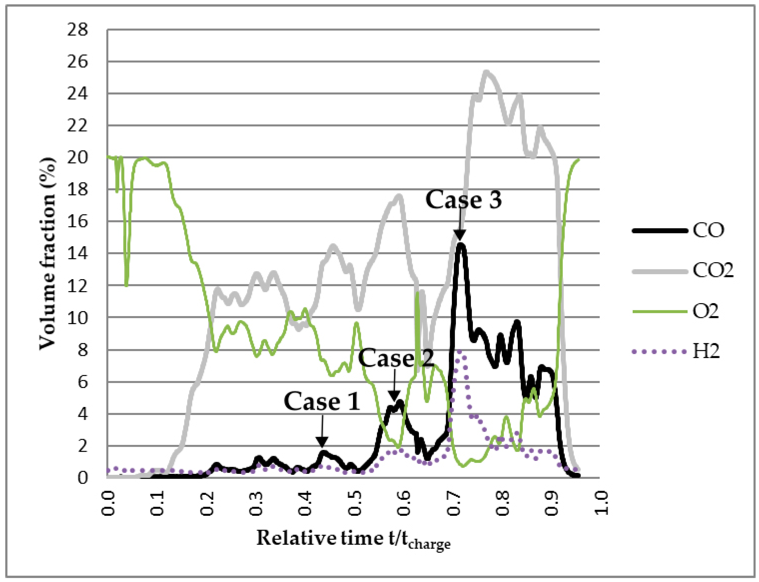
2.5. Case Studies

Before acquiring the off-gas measurements, four cases were studied, as shown in

Table 4. The average volume mass fraction of species for four different cases.

Case	CO Mass Flow Rate (kg·s−1)	Slag Door	Mode
1	0.5	Closed	B3
2	1	Closed (one step reaction)	B + L1
3	1	Open	B + L1
4	1	Closed (O2 removal)	B + L1

. In cases 1 and 2, the simplified oxy-fuel reaction and the first method to exclude oxygen from the main nozzle were used for the B and B+L modes, respectively. In case 3, the air ingress through the slag door is considered. In case 4, the oxygen removal from the furnace is taken into account.

The off-gas measurements data were used to reach a concentration of around 50% nitrogen at the outlet. Then, different flow rates of CO were applied in order to reach the gas composition at the outlet which was first estimated using the backward modelling of the gas flow (reverse engineering) [14]. The first method to exclude the main oxygen partially was used in this case. Then, the influence of the variation of the secondary oxygen flow rate on PC was studied.

2.6. Calculation Procedure

ANSYS FLUENT 13.0.0 (Canonsburg, PA, USA) is used to create the geometry, to generate the mesh and to solve the conservation equations. First, a tetrahedral mesh was generated using ANSYS Meshing and then the tetrahedral cells were converted to polyhedral ones in FLUENT. The final number of cells is equal to 2,000,000. The standard k–ε model is applied to describe the turbulent flow. In addition, the Finite Rate/Eddy Dissipation model in FLUENT is used to model the reactions. The SIMPLE algorithm and PRESTO (PREssure Staggering Option) scheme are applied for the pressure–velocity coupling and pressure discretization, respectively.

3. Results and Discussion

The results are divided into two parts. The first part shows different approaches done to model the flow inside the furnace, namely cases 1–4. In the second part, the CO flow rate at the bath was estimated using the predicted gas composition at the outlet [14]. Besides, the variation of the secondary oxygen flow rate was also studied.

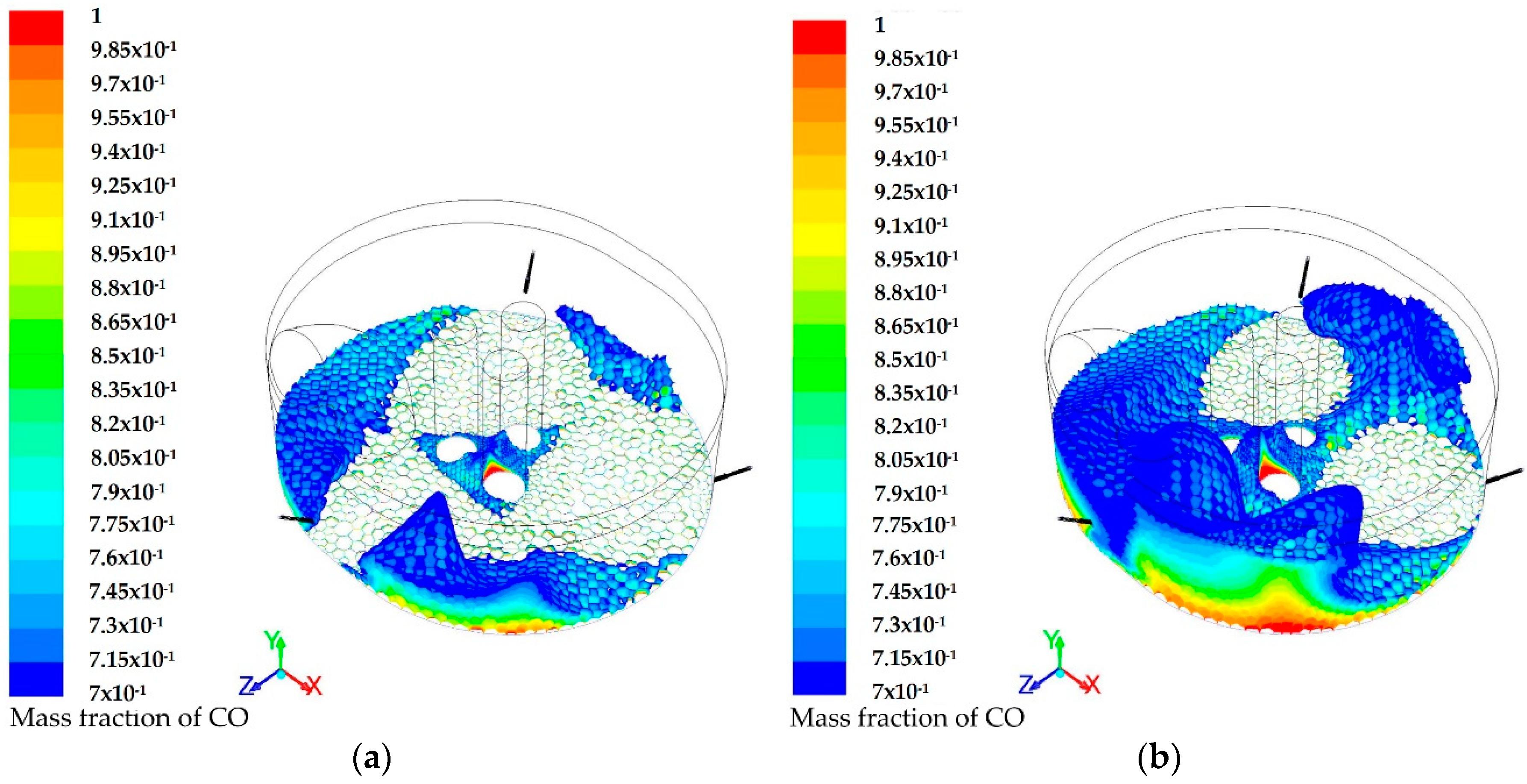
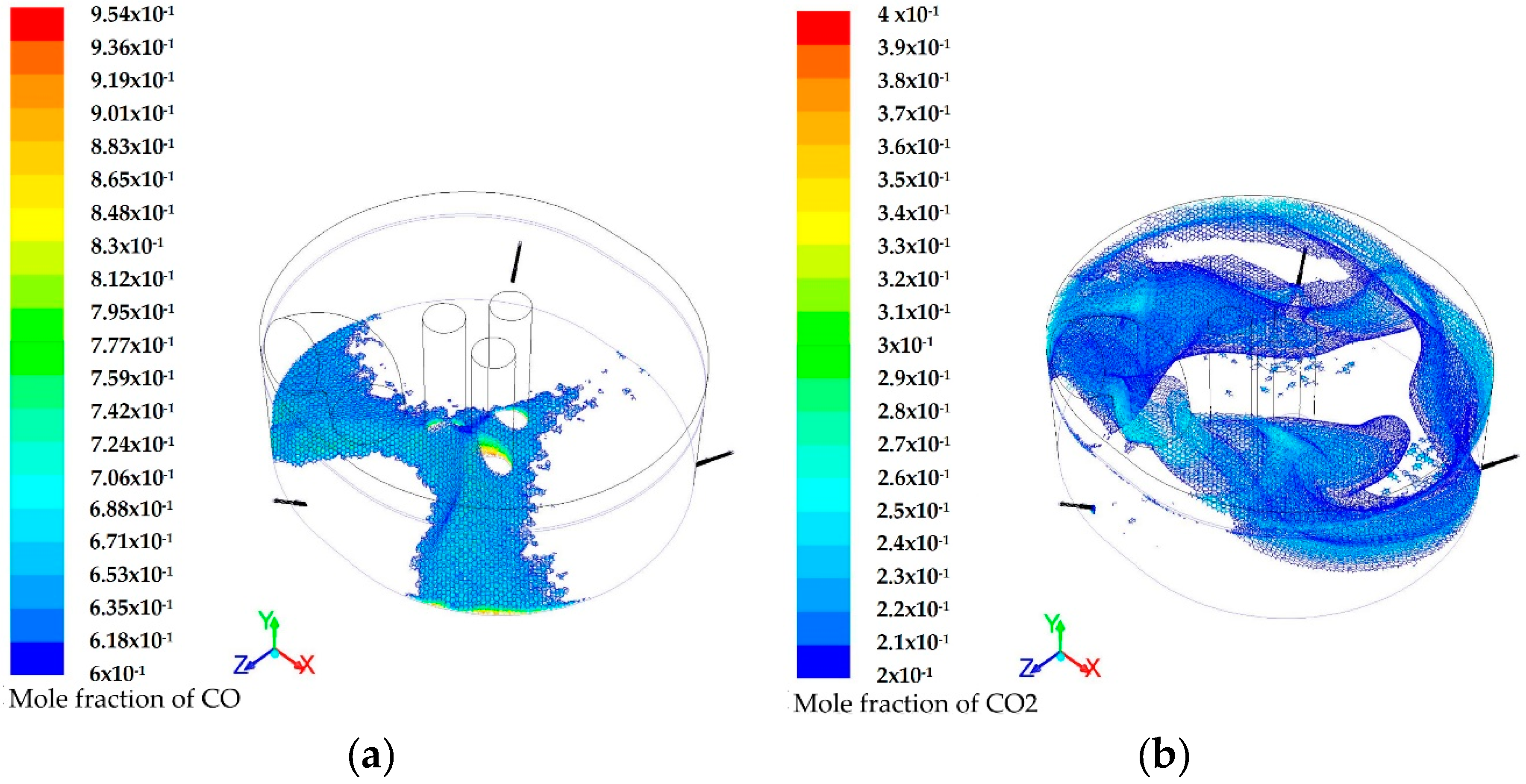
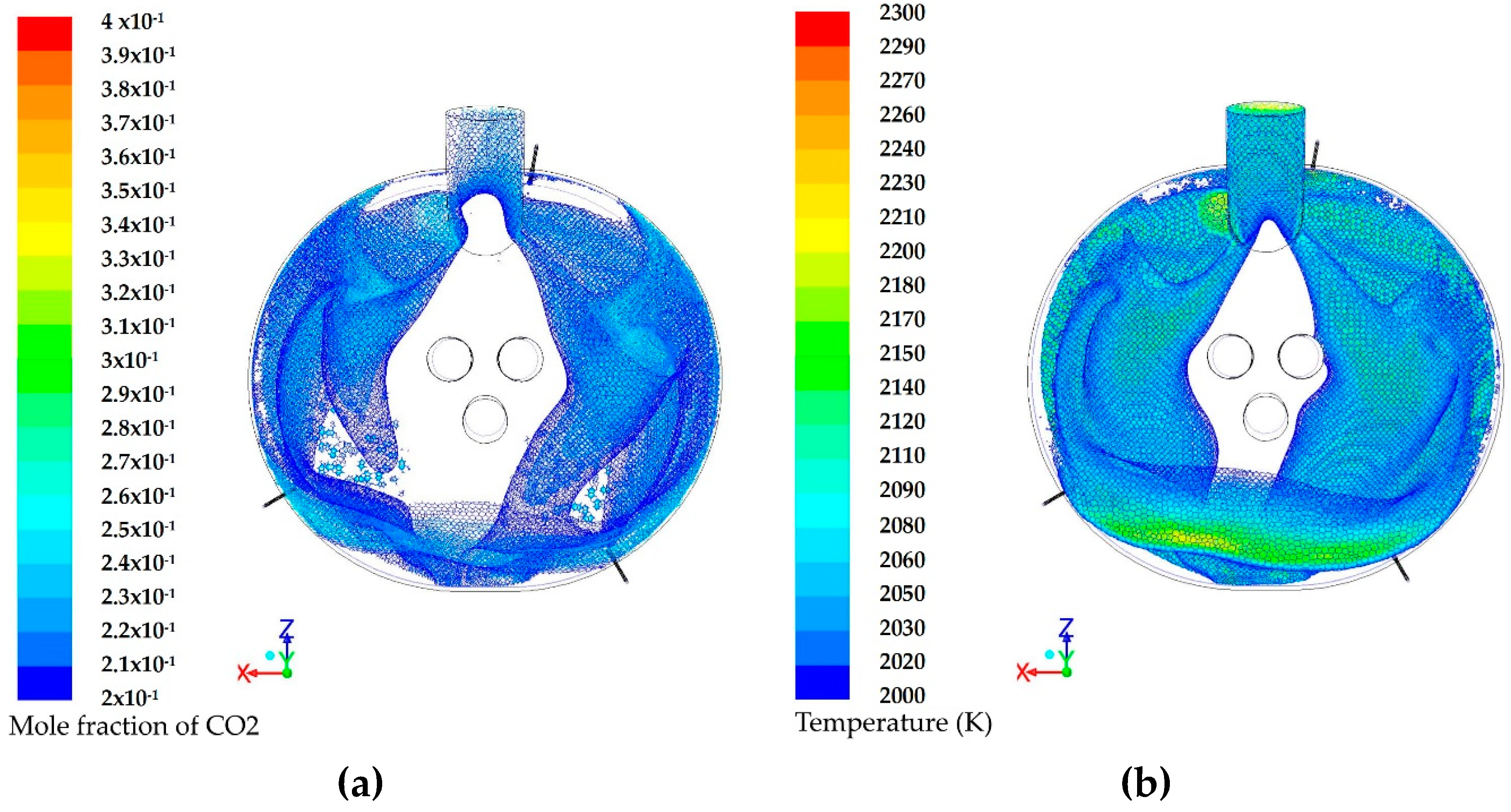
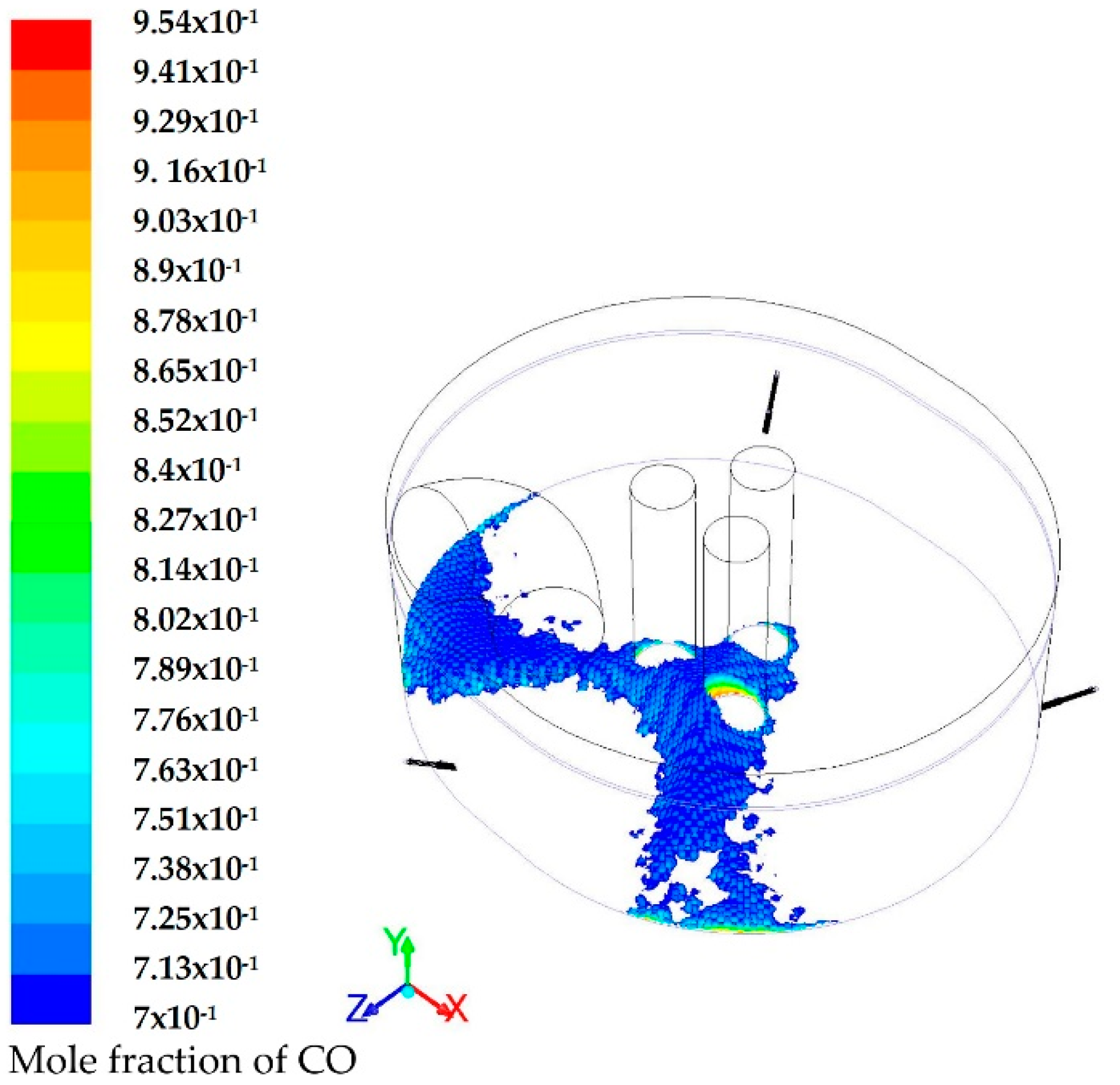
3.1. Modeling of the Reactions Inside the Furnace

Figure 2 shows the high CO concentration ($0.7\le Y_{CO}\le 1$) region inside the furnace in both modes. The concentration of CO is high at the corners between the VLBs and has a maximum value between VLB2 and VLB3.

The highest concentration of CO₂ was observed close to the VLB1 and VLB2, which are located at a further distance from the elbow compared to the VLB3 position. The concentration of CO was higher for the burner + lancing mode compared to the burner mode, Figure 2. This was due to the higher assumed flow rate of CO at the melt surface and the lower flow rate of secondary oxygen in the burner + lancing mode compared to the burner mode. The maximum temperature calculated in case 2 was 2925 K. This high temperature was due to the fact that the endothermic de-PC reaction of CO₂ with carbon in the melt and the electrodes was not considered. The open slag door resulted in a lower maximum temperature of 2429 K, which was due to air leakage into the furnace.

The area weighted average value for each species mass fraction ($\frac{1}{A_{outlet}}\int Y_{i}dA$) at the outlet is shown in

Table 5. The calculated composition of each species at the outlet given in mass fraction.

Case	N2	CO	CO2	PCR
1	-	0.52	0.18	0.26
2	-	0.64	0.13	0.16
3	0.09	0.6	0.14	0.19
4	-	0.55	0.32	0.36

. It is seen that the amount of CO₂ generated was lower for the B+L mode (case 2) compared to the burner mode (case 1). This results in a lower value of the postcombustion ratio (PCR = $\frac{mf C{O}_2}{mf C{O}_2+mf CO}$).

CO₂ concentration at the outlet was about 8% higher when the slag door was open compared to when it was closed, as seen in Table 5. Due to the air leakage from the slag door, the amount of N₂ also increased. Since the NO formation is neglected, the CO combustion by oxygen was overestimated.

The results of the mass removal of oxygen from the bottom of the furnace are shown in Table 5. A higher PCR value was achieved, but this is highly dependent on the sink source and its height from the bath surface.

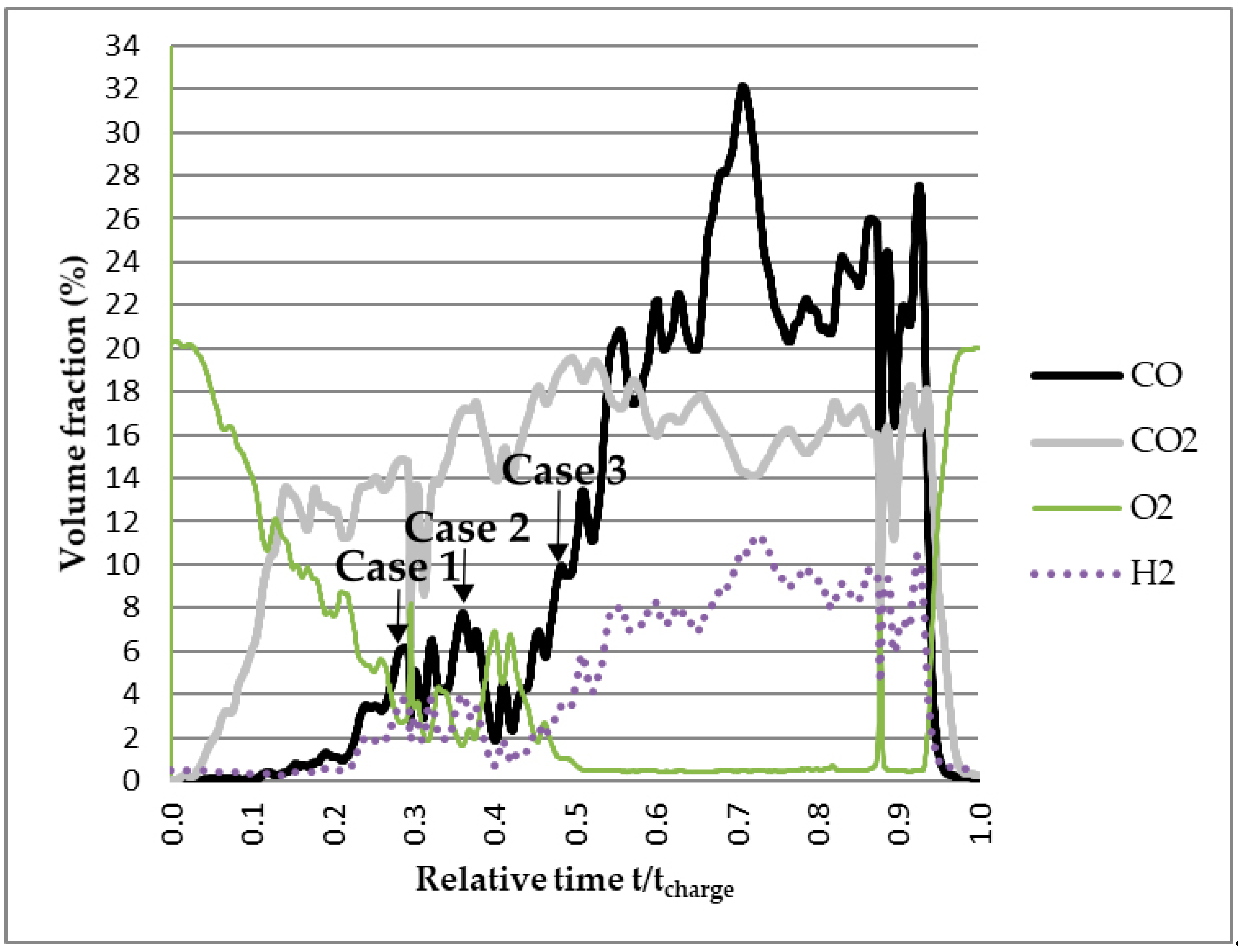
3.2. Modeling the Gas Flow in the Furnace based on the Off-Gas Measurements

In this part, the EAF model was combined with data from off gas measurements to estimate the postcombustion inside the furnace. A gas analysis probe was installed to monitor the off-gas composition at the furnace outlet. The only technically possible place to install the probe was judged to be after the air gap between the furnace elbow and duct system. The air enters through the gap to cool down the off-gas entering the duct. The combined model of the EAF and part of the duct are shown in Figure 3. The outlet surface at the elbow in the EAF was connected to the outlet at the duct. The positions of the tip of the probe and the air gap are shown in Figure 3.

Figure 4 and Figure 5 show the measured off-gas compositions given in volume fraction (%) at the probe position for two charges (charge A and charge B) versus the relative time to the charge time. During each charge, scrap was charged into the furnace and melted.

Since the probe was located after the air gap, first, the off-gas composition at the outlet of the furnace before the air gap is calculated. This was done by using backward modeling of the gas flow inside the duct system [14].

Three cases each were considered for charges A and B during the furnace operation, where CO peaks were observed. These corresponded to 6%, 8%, and 10% for charge A, as shown in Figure 4. Furthermore, 2%, 5%, and 15% CO for charge B, as shown in Figure 5.

The final results of the off-gas composition in mole fraction (equivalent to volume fraction for an ideal gas mixture) at the duct inlet, which meets the composition at the probe spot, are shown in

Table 6. The predicted composition (mole fraction) at the duct inlet for charge A [14].

Case	Composition at the Duct Inlet (mf)				Vin	Pout	Composition at the Probe (Avg. mf)
	CO	CO2	O2	H2			CO	CO2	O2	H2
1	0.14	0.14	10−4	0.04	22	−320	0.06	0.168	0.017	0.033
2	0.2	0.16	10−4	0.07	22	−320	0.082	0.18	0.022	0.069
3	0.2	0.14	10−4	0.09	22	−300	0.11	0.176	0.01	0.076

and

Table 7. The predicted composition (mole fraction) at the duct inlet for charge B [14].

Case	Composition at the Duct Inlet (mf)				Vin	Pout	Composition at the Probe (Avg. mf)
	CO	CO2	O2	H2			CO	CO2	O2	H2
1	0.1	0.12	0.08	0.01	20	−320	0.015	0.18	0.062	0.009
2	0.13	0.15	10−4	0.03	22	−320	0.053	0.173	0.019	0.024
	0.13	0.16	10−4	0.03	22	−320	0.054	0.182	0.019	0.024
3	0.24	0.12	10−5	0.09	22	−300	0.146	0.161	0.007	0.077
	0.25	0.12	10−5	0.09	22	−300	0.155	0.161	0.007	0.077

[14]. The rest of the predicted duct inlet concentrations were around 54% to 67% nitrogen and water. These results were used as the off-gas composition at the outlet in the furnace model.

Table 8. The calculated composition (average mole fraction) at the furnace outlet; burner mode.

Case	Air Flow Rate (Roof) (kg·s−1)	CO Flow Rate (Bottom) (kg·s−1)	N2	CO	CO2	H2O
1	1.5	1	0.44	0.23	0.19	0.07
2	1.5	0.8	0.47	0.18	0.2	0.08
3	1.5	0.6	0.51	0.12	0.21	0.089
4	1.5	0.5	0.52	0.09	0.21	0.095
5	1.8	1	0.48	0.183	0.206	0.069
6	1.8	0.8	0.51	0.13	0.22	0.077
7	1.8	0.7	0.53	0.1	0.22	0.08
8	2	0.9	0.52	0.127	0.22	0.071

shows the results for the off-gas composition at the outlet for different CO flow rates and air flow rates from the roof ring gap for the burner mode. It should be mentioned that no measurements were available to estimate the air flow rate into the furnace.

The result for CO concentration in case 3 (0.12), with a CO flow rate of 0.6 kg·s⁻¹ in Table 8, is in better agreement with case 1 (0.14) in Table 6, which corresponds to the burner mode. In case 4 in Table 8, the flow rate of 0.5 kg·s⁻¹ results in a CO concentration of 0.09 This is in a better agreement with the CO concentration in case 1 in Table 7, which is 0.1. In both cases 3 and 4 in Table 8, the CO₂ concentration is higher compared to case 1 in Table 6 and case 1 in Table 7. As it is mentioned before, the assumption of the simplified oxy-fuel reaction leads to an overestimation of the combustion of CO. Besides, the irreversible reaction (Reaction 2) was applied for the combustion of CO. In reality, CO₂ dissociates to CO and O₂ at high temperatures. The de-PC, due to reaction of CO₂ with carbon in the melt and in the electrodes, was also not modeled. Therefore, it can be concluded that the condition applied for case 4 can correspond to the predicted gas composition in case 1, as seen in Table 7. It should also be mentioned that the unreacted oxygen from the main nozzle (around 0.08 in mole fraction) decreases the ratio of other species at the outlet.

It is seen in Table 8 that the introduction of more air through the roof ring gap, causes the concentration of CO and CO₂ to decrease and increase, respectively.

The results of the outlet composition for the burner + lancing mode (B+L1) are presented in

Table 9. The calculated composition (average mole fraction) at the furnace outlet; burner + lancing mode.

Mode	Case	Air Flow Rate (Roof) (kg·s−1)	CO Flow Rate (Bottom) (kg·s−1)	N2	CO	CO2	H2O
B+L1	1	1.5	0.7	0.46	0.131	0.223	0.069
	2	1.5	0.8	0.45	0.1551	0.219	0.066
B+L2	3	1.5	1.2	0.39	0.24	0.21	0.045
	4	1.2	1	0.37	0.24	0.2	0.05

, cases 1 and 2. The calculated concentration of CO in case 1 in Table 9 is in good agreement with case 2 in Table 7, which is equal to 0.13. The amount of CO₂ is 40% higher than the predicted value in Table 7. This can be explained by the same reasons which are mentioned above for the burner mode.

A high level of CO is observed for case 3 in Table 7. This corresponds to the burner + lancing mode 2 (B+L2), where the carbon lancing starts. The concentration of CO is estimated to be higher than the CO₂ concentration. This is due to the fact that less air is infiltrated during this mode (lower concentration of nitrogen) compared to the previous cases. The results of the outlet composition for the burner + lancing mode (B+L2) are presented in Table 9, cases 3 and 4. The predicted CO value of around 0.24 in Table 9 is in good agreement with the CO concentration values of 0.24 and 0.25 at the duct inlet in case 3, Table 7.

The CO flow rates and air flow rates that resulted in the best agreements are used to compare the influence of the flow rate of the secondary oxygen on PC. The results for the B3 and B+L1 modes are presented in

Table 10. The calculated composition (mole fraction) at the furnace outlet for different secondary oxygen flow rate adjustments for the burner mode with air flow rate of 1.5 kg·s⁻¹.

Case	CO Flow Rate (kg·s−1)	Secondary Oxygen Flow Rate (kg·s−1)	CO	CO2	O2	PCR
1	0.6	0.063	0.12	0.209	2 × 10−6	0.58
2	0.6	0.1	0.107	0.228	9 × 10−6	0.68

and

Table 11. The calculated composition (mole fraction) at the furnace outlet for different secondary oxygen flow rate adjustments for the burner + lancing mode with air flow rate of 1.5 kg·s⁻¹.

Case	CO Flow Rate (kg·s−1)	Secondary Oxygen Flow Rate (kg·s−1)	CO	CO2	O2	PCR
1	0.8	0.059	0.156	0.216	1.1 × 10−6	0.581
2	0.8	0.065	0.155	0.219	1.4 × 10−6	0.585
3	0.8	0.07	0.154	0.221	8 × 10−7	0.589
4	0.8	0.1	0.142	0.236	8 × 10−7	0.624

. Table 10 shows that the PCR increases by 17% in the burner mode, when the secondary oxygen flow rate increases by 60% (from 0.063 kg·s⁻¹ to 0.1 kg·s⁻¹). Table 11 shows that the mass flow rate of the secondary oxygen increases by 70% (from 0.059 kg·s⁻¹ to 0.1 kg·s⁻¹), the concentration of CO₂ increases by 9% and the PCR increases by 7%.

For both mentioned modes, the oxygen concentration remains almost unchanged when the secondary oxygen flow rate is almost two times higher than its initial value.

The postcombustion improves the energy efficiency in EAFs when there is scrap left inside the furnace and also when the scrap absorbs the heat released by the PC reaction. Hence, the highest calculated PCR value at the outlet cannot be the representative of an improved energy efficiency in an EAF. The regions inside the furnace with high CO₂ concentrations must be detected.

Figure 6 demonstrates the high CO (0.6 to 0.95 in mole fraction) and high CO₂ concentration regions inside the furnace for a B+L1 case in which the CO flow rate is 0.8 kg·s⁻¹. It can be seen in Figure 6a that a higher combustion of CO takes place at the positions VLB1 and VLB2. However, still, the region at the lower part of the furnace close to VLB3 has the potential to become combusted. The high CO₂ concentration area at the lower zone of the furnace is shown in Figure 6b, which is located between the VLB1 and VLB2 positions. It can be seen in both Figure 6b and Figure 7a that the CO₂ concentration is also high at the roof, which is due to the air flow through the gap where there is no scrap present. The corresponding high temperature regions are shown in Figure 7b.

The high CO concentration region for case 4 in Table 11, with a secondary oxygen flow rate of 0.1 kg·s⁻¹, is shown in Figure 8. This is obviously lower compared to case 1 in Table 11 due to the higher postcombustion ratio.

3.3. Calculation of the Energy Available in Uncombusted CO Gas

The result of the enthalpy and capacity of CO combustion is shown in

Table 12. The estimation of the capacity of combustion of the CO leaving the furnace compared to the capacity of the oxy-fuel reaction in burner and burner + lancing modes.

Condition	Burner Mode	Burner + Lancing Mode
CO (mole fraction)	0.09	0.156
CO mass flow rate (kg·s−1)	0.14	0.39
Enthalpy of CO combustion (kWh·kg−1 of CO)	2.39	2.39
Capacity of CO combustion (MW)	1.19	3.13
CH4 mass flow rate (kg·s−1)	0.06	0.05
Enthalpy of reaction 1 (kWh/mole)	0.24	0.24
Capacity of reaction 1 (MW)	3.35	2.77

. The enthalpy is calculated by assuming that CO reacts with cold oxygen (at 298 K) at a temperature of 1800 K. The enthalpy of CO₂ is calculated at 2000 K [15].

The burner and burner + lancing modes for charge A are taken into account since there is still an amount of scrap available inside the furnace, and there is a potential to use the chemical energy. In the burner case, the composition and flow rate of CO are 0.09 and 0.14 kg·s⁻¹ at the outlet are taken into account. For the burner + lancing case, the composition and flow rate of CO are 0.156 and 0.39 kg·s⁻¹ at the outlet, respectively. The capacity of CO combustion is calculated as 1.19 and 3.13 MW, and the capacity of the oxy-fuel reaction (Reaction 1) is calculated as 3.35 and 2.77 MW for the burner and burner + lancing modes, respectively. These results show that a considerable amount of energy is available through the PC compared to the energy contribution from the oxy-fuel reaction.

4. Conclusions

The present work focused on investigating the capability of postcombustion in an EAF by adjusting the oxygen flow rate into the furnace. The postcombustion inside an electric arc furnace was developed using CFD. The modeling results were combined with off-gas measurements. The predicted off-gas composition at the furnace outlet [14] was used to estimate the flow rate of CO inside the furnace. The effect of the secondary oxygen flow rate on postcombustion was studied based on the estimated CO flow rates. The results illustrate that when the secondary oxygen flow rate increases by 60% and 70%, the PCR increases by 17% and 7% for the burner and burner lancing modes, respectively.

The capacity of the uncombusted CO in the burner and burner + lancing modes were found to be 1.19 MW and 3.13 MW, respectively. Thus, there is a potential to increase the energy supply to the furnace substantially.

References

1. Grant, M.G. Principles and strategy of EAF post combustion. In Proceedings of the 58th Electric Furnace Conference and 17th Process Technology Conference, Orlando, FL, USA, 12–15 November 2000. [Google Scholar]
2. Januard, F.; Bockel-Macal, S.; Vuillermoz, J.C.; Leurent, J.; Lebrun, C. Dynamic control of fossil fuel injections in EAF through continuous fumes monitoring. Revue Métall. 2006, 103, 275–280. [Google Scholar] [CrossRef]
3. Li, Y.; Fruehan, R.J. Computational fluid dynamics simulation of post combustion in the electric arc furnace. Metall. Mater. Trans. B 2003, 34B, 333–343. [Google Scholar] [CrossRef]
4. Zhonghua, W.; Mazumdar, D.; Mujumdar, A.S. Optimization of post combustion in an electric arc furnace for advanced steelmaking. In Proceedings of the 3rd International Conference on Processing Materials for Properties 2008, Bangkok, Thailand, 7–10 December 2008. [Google Scholar]
5. Thomson, M.J.; Kournetas, N.G.; Evenson, E.; Sommerville, I.D.; McLean, A.; Guerard, J. Effect of oxyfuel burner ratio changes on energy efficiency in electric arc furnace at Co-Steel Lasco. Ironmak. Steelmak. 2001, 28, 266–272. [Google Scholar] [CrossRef]
6. Chan, E.; Riley, M.; Thomson, M.J.; Evenson, E.J. Nitrogen Oxides (NOx) Formation and Control in an Electric Arc Furnace (EAF): Analysis with measurements and computational fluid dynamics (CFD) modeling. ISIJ 2004, 44, 429–438. [Google Scholar] [CrossRef]
7. Opfermann, A.; Riedinger, D. Energy efficiency of electric arc furnace. In Proceedings of the 9th European Electric Steelmaking Conference, Krakow, Poland, 19–21 May 2008. [Google Scholar]
8. Oseman, A.; Ridgeway, J. Performance of the New VLB System at CMC Steel South Carolina. In Proceedings of the AISTech Conference, St. Louis, MI, USA, 4–7 May 2009. [Google Scholar]
9. Westbrook, C.K.; Dryer, F.K. Simplified reaction mechanisms for the oxidation of hydrocarbon. Combust. Sci. Technol. 1981, 27, 31–43. [Google Scholar] [CrossRef]
10. ANSYS FLUENT. Theory and User’s Guide, Release 13.0.0. In Southpointe, 275 Technology Drive; ANSYS FLUENT: Canonsburg, PA, USA, 2010. [Google Scholar]
11. Milewski, J.; Świrski, K.; Santarelli, M.; Leone, P. Advanced Methods of Solid Oxide Fuel Cell Modeling; Springer: London, UK, 2011; p. 201. [Google Scholar]
12. Magnussen, B.F.; Hjertager, B.H. On Mathematical Models of Turbulent Combustion with Special Emphasis on soot Formation and Combustion. Symp. Combust. 1977, 16, 719–729. [Google Scholar] [CrossRef]
13. Peters, A.A.F.; Weber, R. Mathematical modeling of a 2.25 MWt swirling natural gas flame. Part 1: eddy break-up concept for turbulent combustion; probability density function approach for nitric oxide formation. Combust. Sci. Technol. 1995, 110, 67–101. [Google Scholar] [CrossRef]
14. Arzpeyma, N.; Ersson, M.; Jönsson, P.G. Modeling of Post Combustion inside the Off-Gas Dust System of the Ovako Electric Arc Furnace. In Proceedings of the 10th International Conference on CFD in Oil & Gas, Metallurgical and Process Industries SINTEF, Trondheim, Norway, 17–19 June 2014. [Google Scholar]
15. Toulouevski, Y.N.; Zinurov, I.Y. Innovation in Electric Arc Furnaces; Springer: Heidelberg, Germany; Dordrecht, The Netherlands, 2010. [Google Scholar]
Figure 1. (a) The virtual lance burner (VLB) domain; right: front view of the outlet and left: side view; (b) the whole computation domain of the electric arc furnace (EAF) model.
Metals 09 00547 g001
Figure 2. High CO concentration region (in mass fraction) in (a) burner mode; (b) in burner + lancing mode.
Metals 09 00547 g002
Figure 3. The combined model of the duct system and EAF model.
Metals 09 00547 g003
Figure 4. Off-gas composition versus relative time (t/tcharge) for the charge A. Note that the gas mixture also includes N2.
Metals 09 00547 g004
Figure 5. Off-gas composition versus relative time (t/tcharge) for the charge B. Note that the gas mixture also includes N2.
Metals 09 00547 g005
Figure 6. (a) High CO concentration region (in mole fraction) and (b) high CO2 concentration region (in mole fraction); burner + lancing mode.
Metals 09 00547 g006
Figure 7. (a) High CO2 concentration region (in mole fraction) and (b) high temperature region (K); top view of the furnace; burner + lancing mode.
Metals 09 00547 g007
Figure 8. High CO concentration region and (in mole fraction) for case 4 in Table 11 (secondary oxygen mass flow rate of 0.1 kg·s−1).
Metals 09 00547 g008