Abstract
The ultrasonic phased array total focusing method (TFM) has the advantages of high imaging resolution and high sensitivity to small defects. However, it has a long imaging time and cannot realize near-distance defect imaging, which limits its application for industrial detection. A sparse-TFM algorithm is adopted in this work to solve the problem regarding rapid imaging of near- distance defects in thin plates. Green’s function is reconstructed through the cross-correlation of the diffuse full matrix captured by the ultrasonic phased array. The reconstructed full matrix recovers near-distance scattering information submerged by noise. A sparse array is applied to TFM for rapid imaging. In order to improve the imaging resolution, the location of active array elements in the sparse array can be optimized using the genetic algorithm (GA). Experiments are conducted on three aluminium plates with near-distance defects. The experimental results confirm that the sparse-TFM algorithm of Lamb waves can be used for near-distance defects imaging, which increases the computational efficiency by keeping the imaging accuracy. This paper provides a theoretical guidance for Lamb wave non-destructive testing of the near-distance defects in plate-like structures.
1. Introduction
Ultrasonic phased arrays have been widely used in industries due to its strong flexibility and high imaging resolution. It has become a research hotspot in the field of ultrasonic non-destructive testing [1,2]. Compared to the traditional single-chip ultrasonic testing, the ultrasonic phased array transducer is composed of several independent elements. By changing the pulse emission time of a single element according to a certain time sequence, the ultrasonic waves emitted by different elements will be superimposed to form a new wave front. Such a technique can perform linear scanning, sector scanning, and dynamic focusing without probe displacement [3]. However, the phased array acquisition system has some physical limitations. According to the superposition theorem, the sound pressure at any point in the sound field is equal to the superposition of radiated sound pressure at each point on the sound source. On the one hand, there is an obvious interference effect in the sound field near the sound source. The sound pressure amplitude in this area presents an obvious oscillation. On the other hand, the impulse response received by the transducer includes not only the scattering information from the transmitter to the receiver, but also the ultrasonic reverberation inside the transducer. This problem is complicated by the nonlinear saturation from electronic and mechanical crosstalk due to the compact array of elements. For all of the above reasons, part of the signal directly captured by the phased array will appear in the near-field blind region within millimeters of the surface.
Defects buried near the surface are one of most important problems affecting the quality of plate metals. Various near-distance defect detection techniques are widely desired and applied in industrial scenarios [4]. The introduction of wedges between the transducer and specimen can mitigate the near-field effects of the transducer and prevent near-distance defects information from being masked in the near-field range. However, due to the presence of sound beam transmission at the wedge–specimen interface, the energy loss during the sound propagation leads to the defect quantification error or even missed detection. This will reduce the detection reliability. Meanwhile, as the ultrasonic wave propagates in the bounded medium for some sufficiently long time, a quasi-uniform diffusion field is obtained after multiple scattering and reflection events [5]. The generation of the diffusion field provides a great opportunity for near-distance defect detection. The concept was originally used in the field of room acoustics, and then in the analysis of acoustic emission signals. For a 3D diffused noise field, the derivative of the sound field cross-correlation received by the two receivers is proportional to the sum of the causal Green’s function and the anti-causal Green’s function between the two points in the time domain. So far, Green’s function recovery theory has been increasingly used in the fields of ultrasound, structural health monitoring (SHM), seismology, and so on [6,7,8]. Lobkis et al. measured the thermal noise diffusion field in a closed aluminum cavity and obtained the time domain Green’s function between the two receivers through cross-correlation processing [9]. Compillo recorded seismic coda information between two stations and found the group velocities and the polarization characteristics of Rayleigh and Love waves by cross-correlating the coda of seismic events [10]. The cross-correlation of ambient noise within a diffuse field will reproduce the Green’s function between two receivers. This method provides a way to achieve passive imaging using only ambient noise without any external source. Chehami carried out experiments based on the reverberation of an elastic thin plate, indicating that the defect location can be localized by using ambient noise, which provides a theoretical basis for defect imaging [11].
In 2005, the total focusing method (TFM) algorithm was first introduced to defect detection by Holmes [12]. TFM for ultrasonic phased array imaging is a signal post-processing algorithm, which excites each element independently and sequentially while reception is performed by all the elements. It enables one to focus on every specified point within the imaging region using data acquired from full matrix capture (FMC) mode. By taking advantage of the maximum available information for each point, this method has better detection sensitivity and resolution compared with the standard scanning technique. Some researchers even called TFM the “golden rule” algorithm in ultrasonic phased array testing. However, with the increase of the array element number, this method becomes inefficient with massive data processing during TFM imaging. It is still difficult to achieve real-time monitoring in industries when using a large-scale array.
This problem can be solved by selecting only a few elements according to certain rules for data volume reduction and effective imaging. Sparse array was widely used in the medical ultrasonic field as a powerful method to improve efficiency [13]. In many applications, the sparse arrays should be able to generate a specified beamwidth while keeping an allowable peak sidelobe level (PSL). Various optimization algorithms have been proposed for designing a sparse array [14,15]. In order to obtain single or multiple nulls at specific directions while maintaining a low sidelobe level, the harmony search (HS) algorithm was applied to adjust the amplitude, phase, and position of a linear array [16]. Trucco designed the two-dimensional sparse array for underwater three-dimensional imaging with a simulated annealing (SA) method. However, sparse arrays with arbitrary aperture and sparse rate cannot be achieved using this method [17]. Murino used a simulated annealing algorithm to reduce the sidelobe level by adjusting the position and amplitude of elements [18]. A two-layer medium corrected sparse-TFM algorithm was developed by Hu et al. in 2017, which can increase the computational efficiency while maintaining a relatively low error for the arc-distributed hole imaging [19]. However, considering the energy loss caused by wedge coupling, it may mislead the defect detection in serious cases. Haupt was the pioneer in introducing the genetic algorithm (GA) into array design to get the optimal or sub-optimal solution within the range of iteration times through continuous crossover and mutation [20]. In the field of defect identification, GA is one of the most popular optimization techniques used for sidelobe level reduction because it searches through the total solution space and can find the optimal solution globally over a domain [21].
A sparse-TFM imaging method with Lamb waves is adopted in this work to achieve rapid imaging of defects that are near the transducer array via direct contact measurements. The near distance means that defects are located in the near field of the ultrasonic phased array and satisfies the near field calculation formula. Due to its low sound absorption, aluminum is a suitable material for diffuse field measurements. Experiments are carried out on aluminium plates containing near-distance holes. The phased array probe is placed on its side to excite S0 mode Lamb waves. First of all, the FMC mode of a phased array probe was used to obtain the diffuse full matrix after data interception. Based on the classical theory of Green’s function, a full matrix containing the near-distance scattering information obscured by the noise can be obtained through cross-correlation of a diffuse full matrix. Second, it turns out that a hybrid full matrix formed by combining the reconstructed matrix with the directly captured full matrix reduces the background noise, and allows for effective near-distance imaging. In order to improve the spatial resolution and efficiency of imaging, GA is applied to optimize the element layout combining the hybrid full matrix. Finally, rapid imaging of near-distance defects in thin plates is achieved using a sparse-TFM algorithm.
2. Theory for the Sparse-TFM Imaging Using the Diffuse Field Information
2.1. Green’s Function Response Recovery
For a phased array transducer with N elements, each element is excited sequentially. The echo signals received by all elements at each transmission are stored to obtain the full matrix data set. Recording from time zero, the directly captured full matrix data with a long enough window length is denoted as , where and correspond to the transmitting and receiving sensors, respectively. Affected by the near-field blind region, the early defect information is completely submerged in the noise with a large amplitude, which cannot be applied to the subsequent near-distance defect imaging.
In fact, near-distance information exists not only in the obscured region, but is also implicitly contained throughout the diffuse field. The diffuse full matrix is from the signal of time window T after a period of time . The larger the time window T of the interception signal, the better the imaging quality of the reconstruction matrix, but at the cost of a longer computing time. The delay time needs to be determined according to the actual diffusion rate and the signal-to-noise ratio. A smaller cannot satisfy the characteristics of a diffusion field and a larger is not conducive to the recovery of early information due to the complex information of diffusion field. In order to effectively recover the Green’s function between two points by using the cross-correction method of the diffusion field, the statistical average of the cross-correlation between two points in the time domain for an N elements array can be expressed as:
A reconstructed Green’s function matrix derived from the Equation (1) is given by:
As a result of the limited number of phased array elements, the recovery of Green’s function is always imperfect and has a lower accuracy than that of the signal directly obtained. Therefore, the reconstructed Green’s function matrix is only approximately equal to the directly captured full matrix . Although the reconstruction method can be used to obtain the near-distance information more accurately, the later time information is better acquired by using the traditional direct measurement method. By combining the two methods and adding appropriate weight coefficients, the most favorable hybrid full matrix for imaging can be obtained as [22]:
where represents the transition time after removing the nonlinear saturation effect of the reconstruction matrix, the parameter is evaluated as the first scattering response information, is the bottom wave time of the tested specimen, and is the smoothness parameter during the transition.
2.2. Sparse-TFM Imaging
TFM allows the beam to be focused at every point in the imaging region, utilizing all the information in the full matrix of the array data to achieve high-resolution imaging for accurate defect location and quantitative analysis. Taking a conventional rectangular specimen as an example, the coordinate system is established as shown in Figure 1. The ultrasonic array transducer is coupled to the specimen. The x-axis is the moving direction of the probe on the surface of the specimen and the z-axis is the depth direction of the specimen.
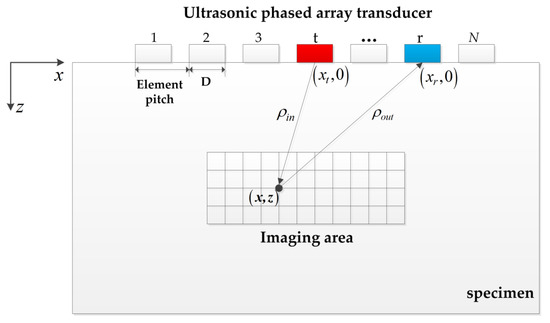
Figure 1.
The schematic diagram of TFM imaging.
The TFM post-processing algorithm first discretizes the imaging area into grid points, and then sums the signals from all elements in the array to synthesize a focal point at each point in the grid. Assuming is a pixel in the grid, the intensity of the image at any point can be calculated as follows:
where N is the number of elements, c is the group velocity of the Lamb wave propagating in the specimen, is the receiving signal of element r while the element t transmits, and and are the coordinates of the transmitting and receiving elements, respectively.
The TFM can be applied to post-processing in nondestructive testing while the computation time is the only limiting factor to processing large amounts of full matrix data. Sparse-TFM is adopted in this work to solve this problem by reducing the number of active transmitting or receiving elements, which is mainly divided into two parts: optimization of the sparse array and TFM imaging. The former is to obtain the optimal or approximate solution of the sparse array distribution in the whole range, while the latter is the process of imaging based on the sparse matrix data. So far, derived from the genetic and evolutionary laws of the biological evolution process, GA is widely used to solve global optimal solution problems. In this paper, the fitness function of GA is constructed based on the minimum sidelobe criterion, and the optimal sparse array distribution is determined within the maximum evolution algebra by the selection, crossover, and mutation operations.
In order to remove image artifacts caused by a sparse transmission or receiving aperture, the effective elements can be weighted to make the effective aperture of the sparse array consistent with that of the full array [23]. In practice, the total effective aperture is obtained by superimposing the effective apertures resulting from individual transmissions at different times, which is shown in Equation (6):
where is the number of transmitting elements, and is the convolution operator. and are the position distribution functions of the transmitting and receiving array elements at the element t excitation, applied with weighting functions and , respectively.
In this paper, for convenience, only the weighting function of the receiving elements is considered by setting for all transmitting elements. Finally, with the aim of imaging the near-distance defects in the target area, the hybrid matrix is substituted for the directly captured matrix. The expression for the sparse-TFM algorithm is shown in Equation (7) [24]:
where and are the total number of transmitting and receiving elements of the sparse array, respectively.
3. Experiments
As shown in Figure 2a, the experimental system was composed of a commercial phased array controller (Multi2000, M2M Inc., France), a computer with a Core E5 CPU and 128 GB RAM, a 1L16-2.0 20 phased array transducer, and three aluminum plates. The aluminum plate was 300 mm 150 mm 1 mm in size with four circular holes. In this paper, three experiments for specimens with different defect were carried out. The relative position of transducers and defects is shown in Figure 2b–d. Specimen 1, including defects parallel to the top edge of aluminum plate, is shown in Figure 2b. Specimen 2, including defects inclined along the top edge of the aluminum plate, is shown in Figure 2c. In specimens 1 and 2, each defect had a diameter of 2 mm and was 10 mm away from the top edge of the aluminum plate. Specimen 3, including defects with different diameters, is shown in Figure 2d. The diameter of each defect in specimen 3 was 1, 3, 5, and 7 mm, respectively, and the distance between the center of each defect and the top edge of the aluminum plate was 40 mm.
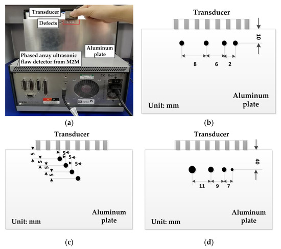
Figure 2.
Schematic of the experimental setup and diagram of defects and transducer position: (a) experimental setup of specimen 1, (b) the relative position of transducers and defects in specimen 1, (c) the relative position of transducers and defects in specimen 2, and (d) the relative position of transducers and defects in specimen 3.
According to the literature [25], the expression of the near-field length for ultrasonic phased array is , where D is the transducer aperture and is wavelength. A five-cycle sinusoidal tone burst signal from a Hanning window was used as the excitation signal in this paper, and the other experimental parameters are listed in Table 1. The phased array transducer was placed above the aluminum plate as shown in Figure 2, which was suitable to excite the S0 mode Lamb waves with a frequency–thickness product of 1 MHzmm [26,27]. In our test, the group velocity of the S0 mode was about 5300 m/s, and the wavelength of the S0 mode was 5.3 mm. After calculation, and . Therefore, the defects in the aluminum plate were located in the near field, and therefore belong to near-distance defects.

Table 1.
Experimental parameters.
Under the configuration of the above parameters, the full matrix of data was obtained by setting the probe to full matrix acquisition mode. An example of typical signals, for , of each full matrix is shown in Figure 3 for specimen 2. The time window T of each set of signals was , and all signals were normalized. The directly captured signal response with a time length of is shown in Figure 3a. It can be seen that the early signals were almost completely submerged by the noise. The diffuse full matrix intercepted by initiating recording some sufficiently long time, , after transmission, is shown in Figure 3b. The reconstructed Green’s function is shown in Figure 3c, which recovers the near-distance information, and lays the foundation for imaging. A hybrid full matrix that better reflects global information is shown in Figure 3d.
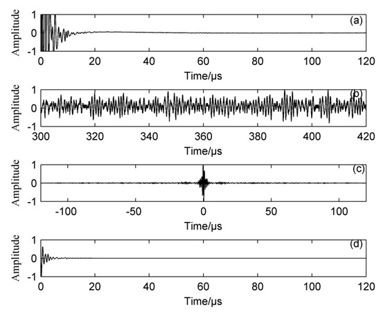
Figure 3.
Example of detection signals with specimen 2 for : (a) directly captured signal response , (b) diffuse full matrix , (c) reconstructed Green’s function, and (d) hybrid full matrix .
4. Experimental Results
4.1. Near-Distance TFM Imaging
Images of the aluminium plates were generated using the TFM, as shown in Figure 4. The directly captured images (Figure 4a,c,e) show a strong area of noise that extends to about 43 mm from the array. The defects of ≈5–40 mm away from the array are submerged by this area. The images produced from the hybrid full matrix are shown in Figure 4b,d,f, which allowed for effective near-distance imaging from a single directly coupled experimental realization. It can be seen that the characteristics of the detected defects were almost identical to their real situation, while the background noise was significantly reduced. Even if the defect had a diameter of only 1 mm, it could be clearly detected.
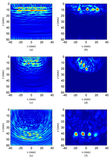
Figure 4.
Near-distance TFM imaging: (a) directly captured full matrix of specimen 1, (b) hybrid full matrix of specimen 1, (c) directly captured full matrix of specimen 2, (d) hybrid full matrix of specimen 2, (e) directly captured full matrix of specimen 3, and (f) hybrid full matrix of specimen 3.
4.2. Sparse Arrays Designed by Using GA
In Figure 4, the near-distance imaging capability of TFM imaging using a hybrid full matrix is demonstrated. However, the entire TFM imaging process is time-consuming, especially when the number of array elements is large. To overcome the above problem, sparse processing was performed on the hybrid full matrix. Considering the influence of active elements on the imaging results, sparse array experiments were carried out with 7, 10, 13, and 16 receiving elements. The sparse receive elements location was optimized using the GA, and the key steps of this algorithm are summarized below [28]:
Step 1. Initialization: Each element in the array is a gene in the chromosome. The values of genes in the active elements are set as 1; otherwise, the values are set as 0. In order to maximize the lateral resolution, the first and the last receiver elements are active. After several experiments, the number of initial groups M and iterations T in this work were set to 30 and 100, respectively.
Step 2. Objective function: To minimize the peak sidelobe level of the sparse array, the fitness function of GA was constructed as follows:
where , is the angle of the incidence of a plane wave, and is the beam steering direction. , where denotes the wavelength of the Lamb wave. is the binary coefficient, is 1 when the element is active, and is 0 when it is inactive. is the peak value of the beam main lobe, and the objective function is defined as: .
Step 3. Selection, crossover, and mutation: The selection, crossover, and mutation algorithm expands the search space of the GA, such that the GA is more likely to get the global optimal value.
Step 4. Stop criteria: The iteration process is terminated if the maximum number of generations is reached.
The optimal location of the active received elements were determined using GA, and three sequences are listed in Table 2.
Table 2.
Sparse arrays designed by GA.
GA, SA, and particle swarm optimization (PSO) are the most mature and widely used in sparse array design. Shi et al. proved that the SA algorithm is better than PSO algorithm in 2013 [29]. Therefore, the effects of the application of GA and SA algorithms are considered and compared. Taking a sparse array with seven active elements as an example, sparse-TFM imaging was performed on the non-optimized array, optimized array of GA, and SA. The comparison results are shown in Figure 5. Comparing Figure 5a and Figure 5b, it appears that the image quality of the second one was better than that of the first. Indeed, it presents fewer artifacts and side noise, especially around the defects. Comparing Figure 5b and Figure 5c, the optimized array using GA presented a better image quality at the same number of iterations. The optimal element layout had the lowest side lobe peak, which could optimize the energy distribution of the sound field, and to weaken the influence of noise on imaging. This illustrates that the optimization of the sparse array using the GA was necessary for sparse-TFM imaging.
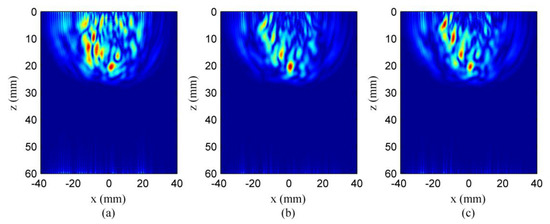
Figure 5.
Sparse-TFM imaging results with seven active elements: (a) non-optimized sparse array; (b) optimized sparse array using the SA, and (c) optimized sparse array using the GA.
4.3. Near-Distance Sparse-TFM Imaging
GA is used to select the element layout of the best effective receiving array elements, and then the corresponding weight functions are performed to obtain the sparse-TFM imaging results, as shown in Figure 6. Figure 6a–c are the imaging results of specimen 1 in different sparse arrays. Figure 6d–f are the imaging results of specimen 2 in different sparse arrays. Figure 6g–i are the imaging results of specimen 3 in different sparse arrays. As the number of receiving elements increased, the image quality was further improved while the artifacts were obviously reduced. This was because the image contrast could be reduced in the case of a high sparse rate due to the influence of the sidelobes. The experimental results detailed above show that clearer defect images with fewer artifacts could be obtained via sparse-TFM using a diffuse field in aluminum plates.
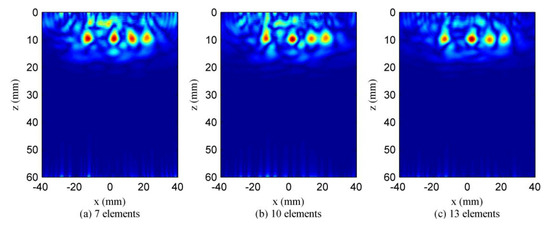
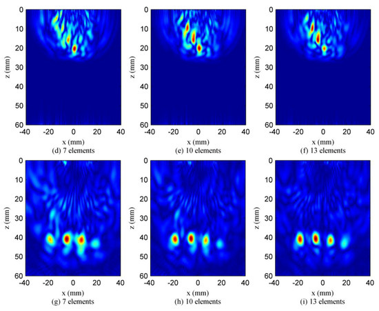
Figure 6.
Sparse-TFM imaging results with varying numbers of receiving elements.
When the number of elements was 13, it was almost the same as the TMF imaging effect. Compared to the 10-element sparse-TFM imaging, one can see that the side lobes and the artifacts near the defect holes in the 7 elements sparse-TFM imaging were greatly increased, but its resolution was acceptable in practical testing. After many experiments, it was shown that when the number of receiving arrays was reduced to 6, some defects could not be imaged due to the sharp decline of energy. Accordingly, it was observed that the fewer combined transmit-receive elements used in sparse-TFM imaging algorithm, the more the resultant sidelobe amplitude was. This is why sidelobes were generated with the TFM imaging, but they can be seen in images generated with the sparse-TFM algorithm.
5. Comparison and Discussion
In order to further analyze the sparse-TFM imaging effect through the cross-correlation of the diffuse field, the array performance indicator (API) and signal-to-noise ratio (SNR) are defined to aid this quantification. API is a dimensionless measurement of the image resolution. The smaller the API value, the narrower the sound beam width and the better the imaging quality [30]. Conversely, the larger the API value is, the wider the ultrasonic beam width will be, which will easily cause aliasing of adjacent defect images and worsen the imaging quality. The expression of API is shown in Equation (9). It is defined as the area, , within which the point spread function is greater than −6 dB down from its maximum value, normalized to the square of the wavelength.
SNR can reflect the overall image quality of the ultrasonic detection image, indicating the relationship between the defect signal and the noise signal [31]. Correspondingly, the expression of SNR is shown in Equation (10):
where denotes the maximum value of the defect signal, and is the average amplitude of the background noise level.
To facilitate the analysis of the imaging results, API, SNR, and computation time of the three experiments for each array were statistically analyzed, as shown in Table 3. The noise suppression was achieved by summing the contributions of different transmitters and receivers. Therefore, the noise level reduced when more receiver elements were used. As the number of array elements increased, the API value decreased, and the SNR value increased continuously. Taking imaging results with specimen 1 as an example, the API value of 7 elements was increased by 26% compared to that of 16 elements. The SNR value was decreased by 5 dB, but the imaging speed was improved by about 2-fold. From these experimental results, it is noted that sparse-TFM imaging could shorten the computation time significantly at the cost of low SNR. Moreover, the image quality of arrays did not have a greater loss under the condition of a certain sparse rates while the imaging efficiency could be greatly improved.
Table 3.
Performance comparison of three specimens for different array.
6. Conclusions
A sparse-TFM algorithm for the near-distance imaging of aluminum plates was presented in this paper, and the influence of sparse receiving elements on computational efficiency and defect quantification accuracy was discussed. The following conclusions can be obtained:
- The feasibility of using the cross-correlation of diffusion field signals from Lamb waves to recover the Green’s function was verified, which is the key process of detecting near-distance defects with an ultrasonic phased array.
- Combining the TFM imaging, a hybrid full matrix formed through an appropriate temporal weighting sum of the reconstruction and conventional full matrix contained the near-distance information and later time information for the imaging of near-distance defects. The defect information presented using this method was almost consistent with the reality, but the calculation was time consuming.
- To maximize the reduction of the data processing times, the sparse-TFM proposed in this paper was similar to the TFM algorithm, but not all elements were used. This work considered the case of a sparse receiver array and a full transmission array, and the sparse-TFM image quality depended on the correct location of active elements in the sparse array to avoid the artifacts and sidelobe noise. GA is an effective optimization method to design sparse receive arrays, which have better performance compared to non-optimized sparse arrays.
Hence, the proposed method allowed for the near-distance defect imaging in thin plates from a single directly coupled experimental realization. It greatly reduced the calculation while keeping a relatively favorable accuracy by reducing the receiving elements. To show the great potential of Green’s function retrieval and sparse-TFM imaging of near-distance defects to inspect plate-like structures, the results presented in this paper have been preliminarily limited to isotropic materials. Since the presented method is based on information processing and optimization algorithm, there is no theoretical obstacle in applying the method to anisotropic materials like the detection of carbon composites, fatigue cracks in flying bodies, etc. These new investigations are now in process.
Author Contributions
Data curation, W.Z.; Formal analysis, G.F.; Investigation, H.Z. (Haiyan Zhang); Methodology, Y.L.; Project administration, H.Z. (Hui Zhang); Writing—original draft, Y.L.; Writing—review and editing, Q.Z.
Funding
The work in this paper is supported by the National Natural Science Foundation of China (Grant Nos. 11874255, 11674214), and the Key Technology R&D Project of Shanghai Committee of Science and Technology (Grant No. 16030501400).
Conflicts of Interest
The authors declare no conflict of interest.
References
- Zhang, C.; Huthwaite, P.; Lowe, M. The Application of the Factorization Method to the Subsurface Imaging of Surface-Breaking Cracks. IEEE Trans. Ultrason. Ferroelectr. Freq. Contr. 2018, 65, 497–511. [Google Scholar] [CrossRef]
- Xiang, Y.; Teng, D.; Deng, M.; Li, Y.; Liu, C.; Xuan, F. Characterization of Local Residual Stress at Blade Surface by the V(z) Curve Technique. Metals 2018, 8, 651. [Google Scholar] [CrossRef]
- Yuan, C.; Xie, C.H.; Li, L.C.; Zhang, F.Z.; Gubanski, S.M. Ultrasonic phased array detection of internal defects in composite insulators. IEEE Trans. Dielectr. Electr. Insul. 2016, 23, 525–531. [Google Scholar] [CrossRef]
- Tian, S.Y.; Xu, K. An Algorithm for Surface Defect Identification of Steel Plates Based on Genetic Algorithm and Extreme Learning Machine. Metals 2017, 7, 311. [Google Scholar] [CrossRef]
- Weaver, R.; Lobkis, O. On the emergence of the Green’s function in the correlations of a diffuse field: Pulse-echo using thermal phonons. Ultrasonics 2002, 40, 435–439. [Google Scholar] [CrossRef]
- Larose, E.; Derode, A.; Campillo, M.; Fink, M. Imaging from one-bit correlations of wideband diffuse wave fields. J. Appl. Phys. 2004, 95, 8393–8399. [Google Scholar] [CrossRef]
- Larose, E.; Roux, P.; Campillo, M. Reconstruction of Rayleigh-Lamb dispersion spectrum based on noise obtained from an air-jet forcing. J. Acoust. Soc. Am. 2007, 122, 3437–3444. [Google Scholar] [CrossRef]
- Sabra, K.G.; Gerstoft, P.; Roux, P.; Kuperman, W.A. Extracting time-domain Green’s function estimates from ambient seismic noise. Geophys. Res. Lett. 2005, 32, L03310. [Google Scholar] [CrossRef]
- Lobkis, O.I.; Weaver, R.L. On the emergence of the Green’s function in the correlations of a diffuse field. J. Acoust. Soc. Am. 2001, 110, 3011–3017. [Google Scholar] [CrossRef]
- Campillo, M.; Paul, A. Long-Range Correlations in the Diffuse Seismic Coda. Science 2003, 299, 547–549. [Google Scholar] [CrossRef]
- Chehami, L.; Rosny, J.D.; Prada, C.; Moulin, E.; Assaad, J. Experimental study of passive defect localization in plates using ambient noise. IEEE-T Special Issue 2015, 62, 1544–1553. [Google Scholar] [CrossRef]
- Holmes, C.; Drinkwater, B.W.; Wilcox, P.D. Post-Processing of the Full Matrix of Ultrasonic Transmit–Receive Array Data for Non-Destructive Evaluation. NDT&E Int. 2005, 38, 701–711. [Google Scholar]
- Austeng, A.; Holm, S. Sparse 2-D arrays for 3-D phased array imaging - design methods. IEEE Trans. Ultrason. Ferroelect. Freq. Contr. 2002, 49, 1073–1086. [Google Scholar] [CrossRef]
- Yang, P.; Chen, B.; Shi, K.R. A novel method to design sparse linear arrays for ultrasonic phased array. Ultrasonics 2006, 44, 717–721. [Google Scholar] [CrossRef]
- Haupt, R.L. Adaptively thinned arrays. IEEE Trans. Antennas Propagat. 2015, 63, 1626–1632. [Google Scholar] [CrossRef]
- Yang, S.H.; Kiang, J.F. Optimization of Sparse Linear Arrays Using Harmony Search Algorithms. IEEE Trans. Antennas Propagat. 2015, 63, 4732–4738. [Google Scholar] [CrossRef]
- Trucco, A. Thinning and weighting of large planar arrays by simulated annealing. IEEE Trans. Ultrason. Ferroelect. Freq. Contr. 1999, 46, 347–355. [Google Scholar] [CrossRef]
- Murino, V.; Trucco, A.; Regazzoni, C.S. Synthesis of Unequally Spaced Arrays by Simulated annealing. IEEE Trans. Signal. Process. 1996, 44, 119–122. [Google Scholar] [CrossRef]
- Hu, H.; Du, J.; Xu, N.; Jeong, H.; Wang, X.H. Ultrasonic sparse-TFM imaging for a two-layer medium using genetic algorithm optimization and effective aperture correction. NDT&E Int. 2017, 90, 24–32. [Google Scholar]
- Haupt, R.L. An introduction to genetic algorithms for electromagnetics. IEEE Antennas Propagat. Mag. 1995, 37, 7–15. [Google Scholar] [CrossRef]
- Du Plessis, W.P.; Bin Ghannam, A. Improved Seeding Schemes for Interleaved Thinned Array Synthesis. IEEE Trans. Antennas Propagat. 2014, 62, 5906–5910. [Google Scholar] [CrossRef]
- Potter, J.N.; Wilcox, P.D.; Croxford, A.J. Diffuse field full matrix capture for near-surface ultrasonic imaging. Ultrasonics 2018, 82, 44–48. [Google Scholar] [CrossRef]
- Lockwood, G.R.; Li, P.C.; O’Donnell, M.; Foster, F.S. Optimizing the radiation pattern of sparse periodic linear arrays. IEEE Trans. Ultrason. Ferroelectr. Freq. Contr. 1996, 43, 7–14. [Google Scholar] [CrossRef]
- Moreau, L.; Drinkwater, B.W.; Wilcox, P.D. Ultrasonic imaging algorithms with limited transmission cycles forrapid nondestructive evaluation. IEEE Trans. Ultrason. Ferroelectr. Freq. Contr. 2009, 56, 1932–1944. [Google Scholar] [CrossRef] [PubMed]
- Sun, F.; Zeng, Z.M.; Jin, S.J.; Chen, S.L. Sound-field of Discrete Point Sources Simulation on Deflecting and Focusing of Near-field of Ultrasonic Phased Array. J. Sys. Simul. 2013, 25, 1108–1112. [Google Scholar]
- Rodriguez, S.; Deschamps, M.; Castaings, M.; Ducasse, E. Guided wave topological imaging of isotropic plates. Ultrasonics 2014, 54, 1880–1890. [Google Scholar] [CrossRef] [PubMed]
- Fan, G.; Zhang, H.; Zhang, H.; Zhu, W.; Chai, X. Lamb Wave Local Wavenumber Approach for Characterizing Flat Bottom Defects in an Isotropic Thin Plate. Appl. Sci. 2018, 8, 1600. [Google Scholar] [CrossRef]
- Haupt, R.L. Thinned arrays using genetic algorithms. IEEE Trans. Antennas Propagat. 1994, 42, 993–999. [Google Scholar] [CrossRef]
- Shi, D.H.; Xi, J.; Zhou, Z.W. Research on optimization method of symmetric thinned planar array. J. Spacecraft TT&C Technol. 2013, 32, 302–305. [Google Scholar]
- Zhang, J.; Drinkwater, B.W.; Wilcox, P.D. Effects of array transducer inconsistencies on total focusing method imaging performance. NDT&E Int. 2011, 44, 361–368. [Google Scholar]
- Velichko, A.; Wilcox, P.D. An analytical comparison of ultrasonic array imaging algorithms. J. Acoust. Soc. Am. 2010, 127, 2377–2384. [Google Scholar] [CrossRef] [PubMed]


© 2019 by the authors. Licensee MDPI, Basel, Switzerland. This article is an open access article distributed under the terms and conditions of the Creative Commons Attribution (CC BY) license (http://creativecommons.org/licenses/by/4.0/).