Abstract
The startup of casting sequences in continuous casting of steel using three different turbulence inhibitors were modeled and simulated through the multiphase volume of fluid model (VOF) in a four-strand tundish. In the actual caster, one of the inhibitors released the liquid steel with a superheat high enough to avoid freezing problems in the outer strands. A second inhibitor improved the flow, yet it yielded steel freezing in these strands. A two-phase air–water system was used to model the liquid steel–air system and the interfaces were tracked by a donor–acceptor principle applied in the computational mesh. These activities led to the design of a third inhibitor. Experimental outcomes and the mathematical simulations agreed remarkably well regarding the velocity of the stream front in the tundish floor and the mass of steel reaching the outer strands. A larger steel mass and a faster stream front helped to completely prevent the steel from freezing in the outer strands. Finally, flow fields during the filling of the tundish using two of these inhibitors were simulated and the results explain the different performances observed experimentally.
1. Introduction
Tundish design consists of the reorientation and guiding of steel flow in order to control its turbulence, to reduce dead zones, and to float out inclusions as much as possible. Most flow control devices (FCDs) consist of arrangements of flow modifiers such as weirs, dams, pads, and turbulence inhibitors (TIs), or a combination of all these devices [1]. The optimal combination of flow modifiers inside of the tundish permits the restructuring of steel flows, causing it to behave as desired, with more plug flows and minimum dead or stagnant regions [2]. This latter requirement is important in order to avoid the formation of steel skulls in the corners of the tundish that facilitate the stripping of the residual steel at the end of a casting sequence. The general procedure to design flow control systems for tundish operations is based on water modeling that determines the residence time distribution (RTD) curves of tracers injected in the inlet, and is sometimes complemented with mathematical simulations [3,4]. Tundish design assumes that the tundish is operating under steady-state conditions. This is true during a good fraction of the casting time of a steel ladle, which explains the great success of the water modeling and mathematical simulation approaches employed in tundish design to date.
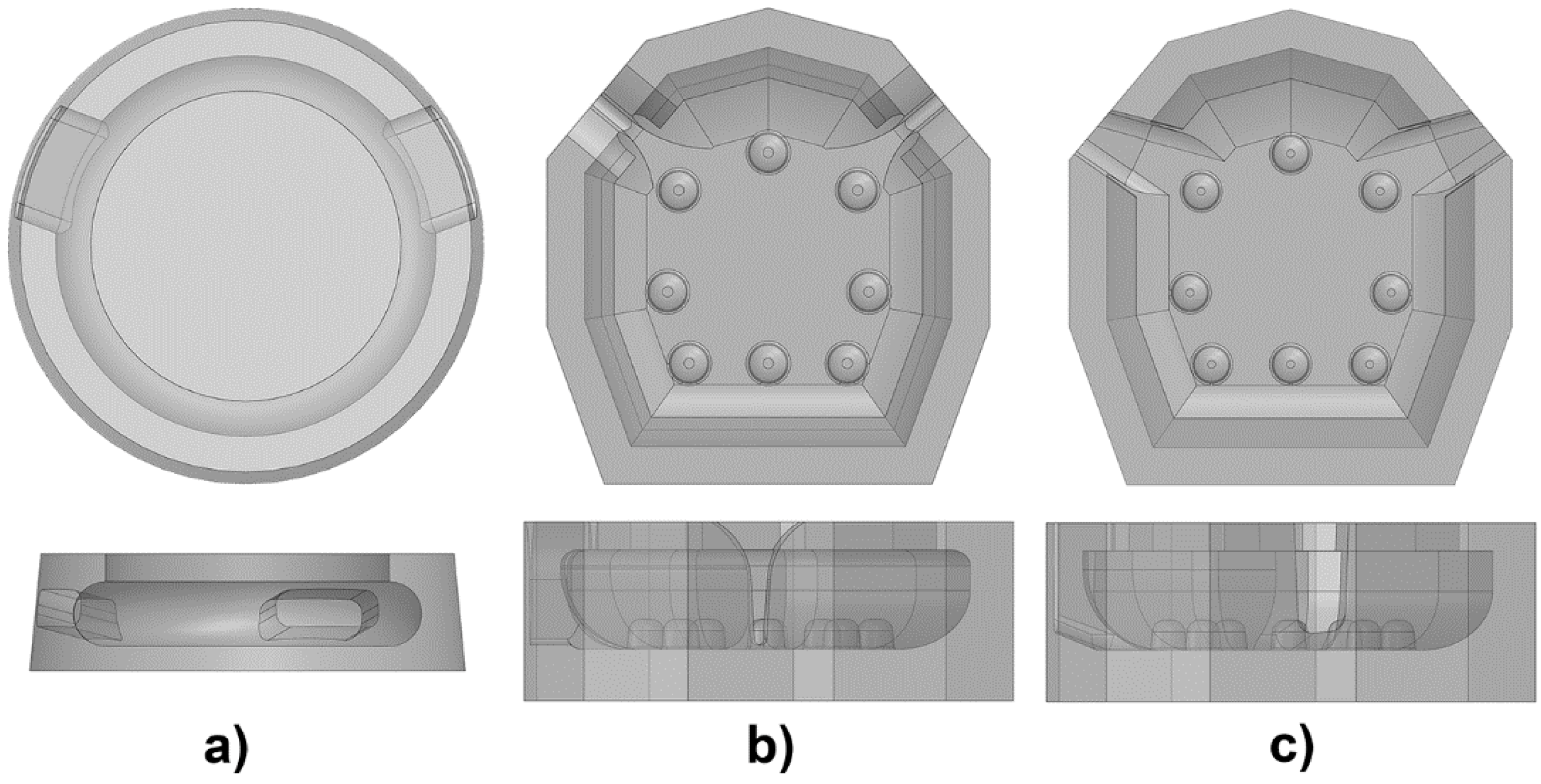
Few reports on tundish design are concerned with designs of flow control systems for transient operations, specifically during ladle change operations, as reported by some researchers [5,6]. Another important unsteady operating condition of the tundish is during the startup of casting sequences, especially when the steel splashing becomes a safety issue in the casting floor. In a previous publication [7], the design of three turbulence inhibitors (TI1, TI2, and TI3, shown in Figure 1) were studied using a 1/3 scale tundish water model, from the point of view of controlling the flow during the startup of casting sequences in a four-strand billet tundish as shown in Figure 2. At the startup of the tundish, whose conditions are reported in Table 1, TI1 delivered streams of steel that reached the two extreme strands without steel freeze-up problems. As the caster required a second of these devices that maintained or, better, improved the floatability of inclusions, a second inhibitor (TI2) was designed and was successful. However, during its trial heats at the caster, TI2 yielded frequent steel freeze-up problems in the two extreme strands of this tundish. Hence, a tradeoff between capability in the floatation of inclusions and avoidance of the freeze-up problems was obtained through a third design (TI3).
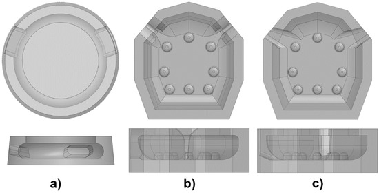
Figure 1.
Turbulence inhibitors tested in this work: (a) TI1; (b) TI2; (c) TI3.
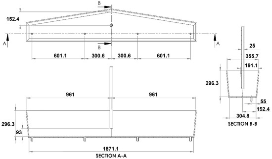
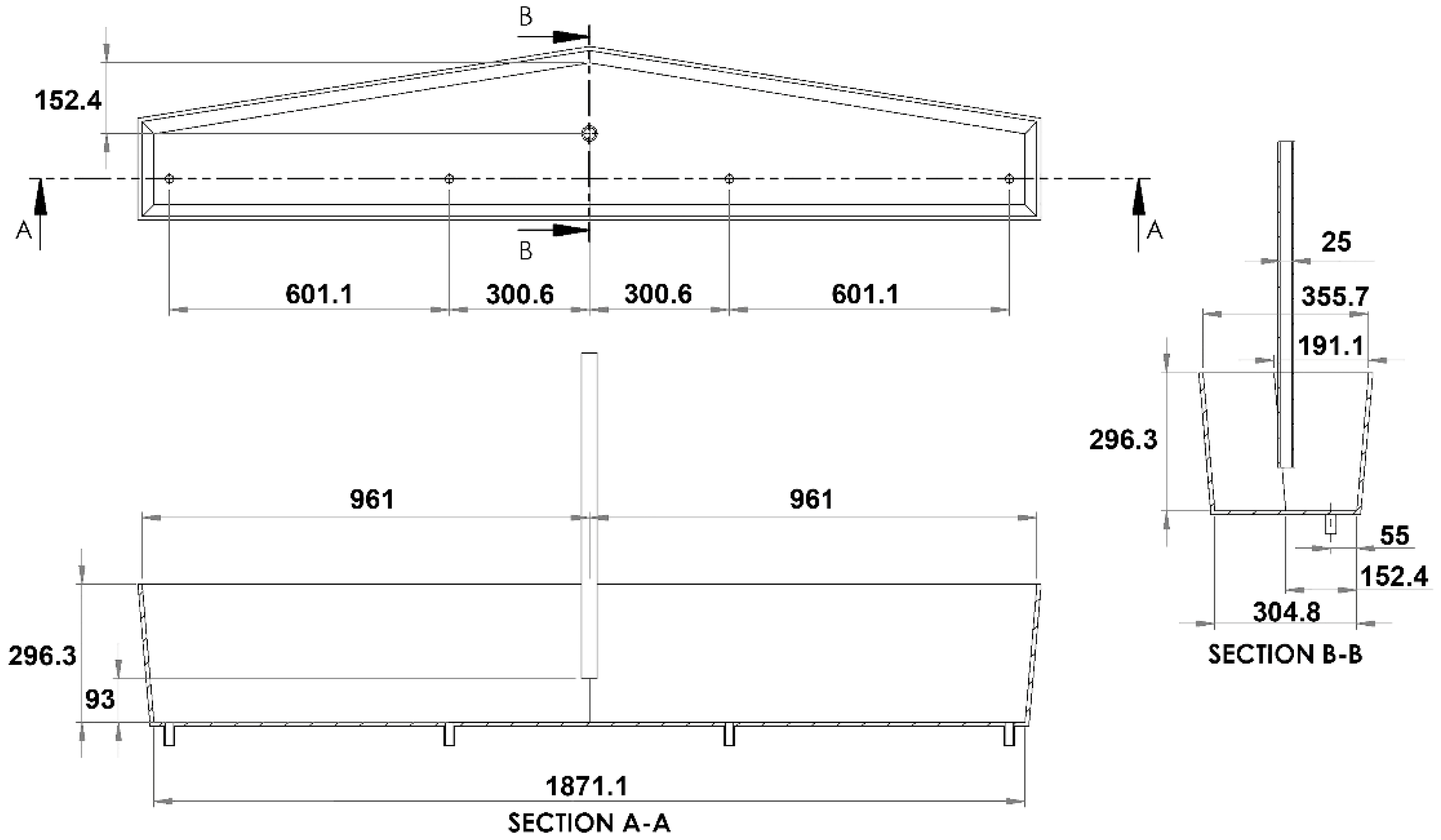
Figure 2.
Dimensions of the tundish in millimeters at 1/3 scale of the actual one.

Table 1.
Operating conditions of the tundish (1/3rd scale) under steady and unsteady conditions (startup of a casting sequence).
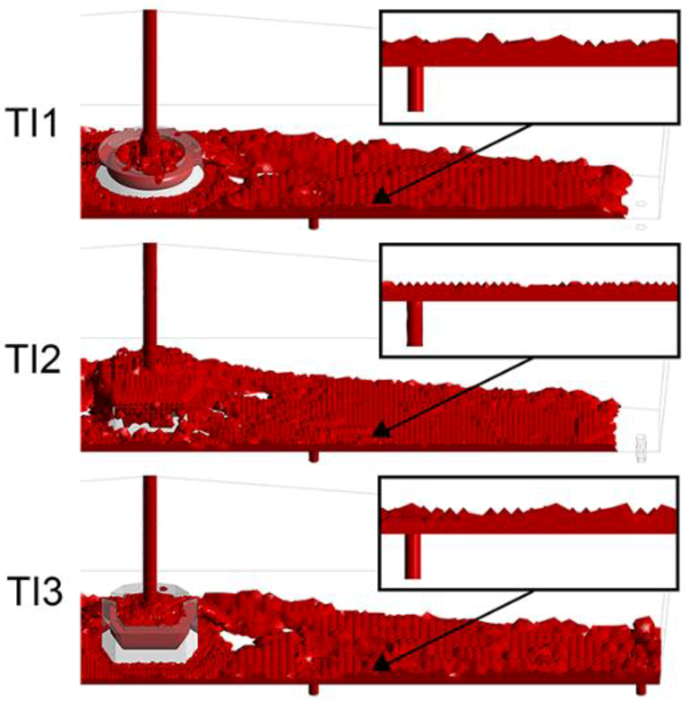
A comparison of the three inhibitors at the startup of the casting was carried out by using red-colored water and the results are reported in Figure 3 [7]. As seen in this figure, the red-colored water reached the extreme strands at about the same time in inhibitors T1 and T3. With inhibitor TI2, the streams did not deliver enough steel at the right speed, and the losses of energy were large enough to create steel freeze-up problems. The present work deals with the rest of the tundish operation after the startup, that is, the tundish filling and the fluid flow dynamics associated with these operations under the conditions reported in Table 1. The basis of the simulation was the water model of the tundish and the inhibitors presented in Figure 1 and Figure 2. Therefore, all the numerical results of fluid flow were related to the flow of water. To translate the velocities from the model to the actual tundish, the following relationship based on the Froude number [8] was employed:
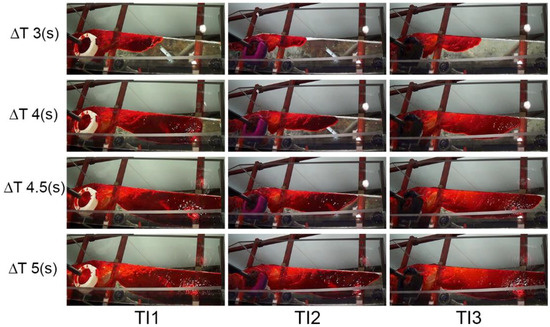
Figure 3.
Streams of liquid water streams at startup operation using different tundish inhibitors.
2. Mathematical Model for the Two-Phase Flow
2.1. The Volume of Fluid Model
The mathematical simulations in this study focused on the startup of the casting to examine liquid splashing and fluid dynamics in the initial tundish filling process. The target of these simulations was to track the gas–liquid interfaces during the initial conditions of turbulence and the interaction of the fluid with the TI at the first instance of the tundish filling. Given the interest outlined here, the most appropriate computing scheme was the volume of fluid (VOF) model [9].For two-phase flows, this model is based on a phase indicator χp(x,y,z,t) that distinguishes if the phase, p, is present in a flow field location with coordinates (x,y,z) at time t. Expressed as a mathematical definition:
When the indicator is averaged over a sufficiently large volume of flow, the fraction volume of phase p is obtained:
The physical properties of the fluids are estimated by simple additive rules:
The continuity equation (without mass exchange among the phases) is:
The velocity–momentum fields shared by the two phases is:
The physical properties are those calculated through Equation (4), and consequently the volume fraction of the phases is implicit in Equation (5). To define the interfaces between both phases, the donor–acceptor formulation of the VOF model was adopted [9]. The tracking of the interfaces was carried out by solving the equation of continuity through an explicit scheme using a Courant number of 0.5:
The contribution of turbulent stresses to the momentum equation is given by the term in Equation (6). Therefore, one of the appropriate models to link Equations (6) and (7) is obtained through the realizable k–ε model [10]. Two additional equations for the turbulent kinetic energy and the dissipation rate of the kinetic energy form parts of the system of equations to be solved [9,10]. The finite volume method was used for the discretization of these equations [11], building a non-structured mesh composed mostly of tetrahedral cells.
To simulate the dispersion of the tracer, the velocity field was calculated from the preceding equations and used in the following mass transfer equation [12]:
where Deff is the effective diffusivity, which is the sum of molecular and turbulent diffusivities, according to:
where D0 is the molecular diffusivity and Sct is the turbulent Schmidt number. Because turbulent flows generally carry mass over an equivalent Schmidt mixing length, this coefficient was assumed to be equal to 1. A concentration-step-type boundary condition was applied at the ladle shroud to simulate the injection of the tracer in the tundish.
2.2. Boundary Conditions and Algorithm of Solution
At the solid surfaces of the tundish system, the logarithmic wall function [8] was employed to link the flow field out of the boundary layer with the flow velocities close to the wall, inside this layer. In the inlet, inside the ladle shroud, a turbulent velocity profile was assumed through the 1/7th law of turbulent flow in pipes [13]. Outlet velocities were also used as boundary conditions in the four strands of the tundish. In the bath surface, a pressure condition was applied. The (Pressure Implicit Splitting Operations) PISO algorithm [9] was employed to solve the set of Equations (4) and (5). At the water–air interfaces, the surface tension force was substituted as a momentum source in the last term, right side of Equation (6), designated by the letter F. The computation of this force (surface tension of water = 0.073 N m−1) was performed using Brackbill’s continuum surface model of [14]. The physical properties used in the model for water density, water viscosity, and surface tension were 1000 kg m−3, 0.001 Pa s, and 0.073 N m−1, respectively. Air density and air viscosity were 1.2 kg m−3 and 18.27 × 10⁻⁶ Pa s, respectively [5,6].
3. Results and Discussion
3.1. Control of Steel Freezing in Outer Strands
To estimate the weights of steel at the instant the streams of water reached the extreme strands, the volumes of the streams of water computed using the VOF model were redefined through software [15]. Later, their respective volumes were scaled up from 1/3rd to full scale. The resulting volumes were multiplied by the density of liquid steel (7100 kg/m3). The results of these operations yielded masses for half the tundish of the liquid stream of 755.41, 617.09, and 762.67 kg for TI1, TI2, and TI3, respectively. These results are presented through the simulated masses of liquid streams with the mathematical model shown in Figure 4. The sizes of the jets flowing through the slits of TI1 and TI3 are apparently larger than those corresponding to TI2, which explains the larger amounts of liquid directed toward the outer streams.
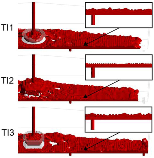
Figure 4.
Initial liquid streams at startup conditions for each TI.
3.2. Control of Tundish Filling Operations
Since the TI3 had the same performance as that of TI1 for startup of the casting sequence and the elimination of the steel freezing problems in the two extreme strands, the next tundish aspect under scrutiny was the fluid dynamics during the filling operation using either TI model. This comparison made it possible, through the analysis of the RTD curves, to elucidate which of the two TIs had better potential to float up inclusions.
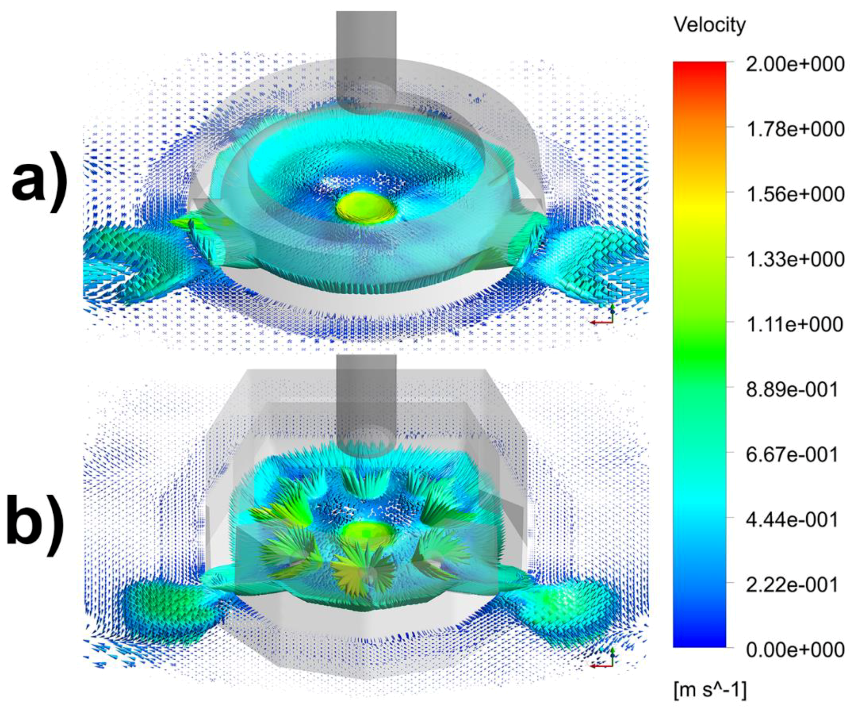
Figure 5 shows the internal velocity fields of the liquid inside TI1 and TI3, respectively. After impacting the bottom, the liquid rose along the curved walls of TI1 with relatively uniform velocities, while in TI3 the presence of the pins at the bottom created local velocity gradients that dissipated the kinetic energy of the liquid. This dissipation was accompanied by a refinement of the turbulent eddies [4]. The jets flowing through the slits of the inhibitors were about the same size, quickly draining the liquid as seen in the photos of the first and third columns of Figure 3, where the inhibitors remained unfilled during the starting operation. Contrary to this performance, TI2 was filled, as seen in the photos of the second column of Figure 3, and this observation is also evident in Figure 4.
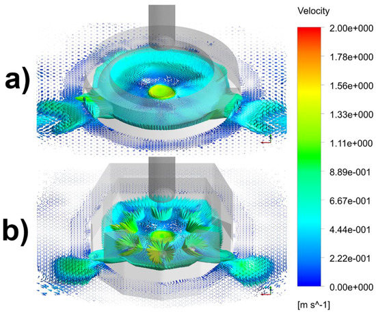
Figure 5.
Numerical velocity fields inside the TIs: (a) TI1; (b) TI3.
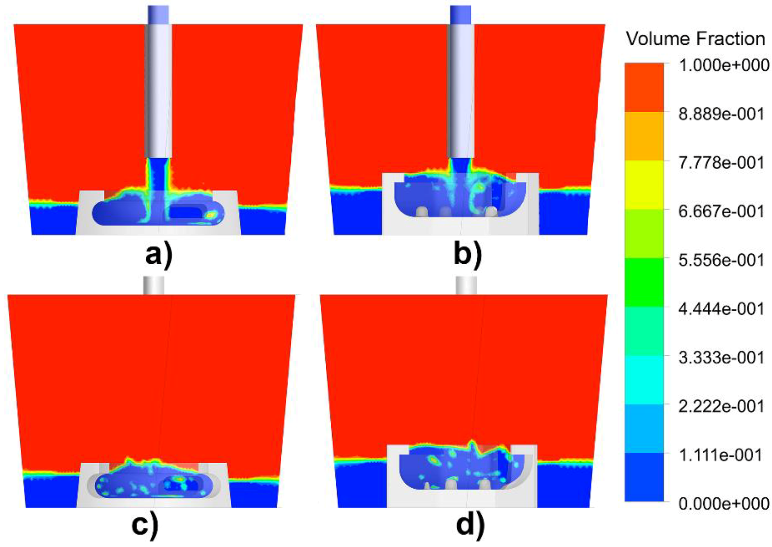
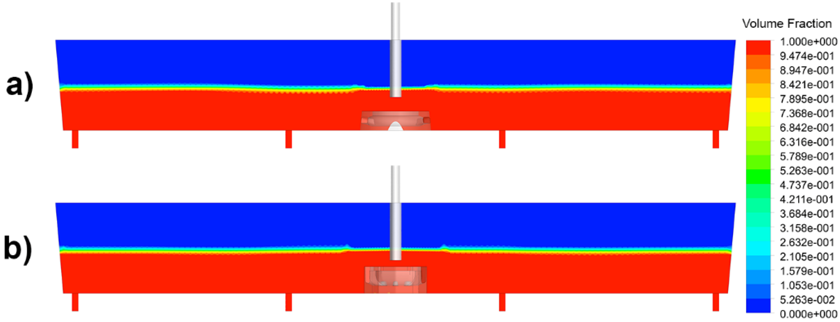
The volume fractions of the air entrained by the entry jets in a plane passing through the axis of the ladle shroud are shown in Figure 6a,b for TI1 and TI3, respectively. Figure 6c,d shows the distribution of volume fractions of phases passing through a plane located between the entry jet and the edge of each inhibitor. Air was entrained through the boundary layer between the liquid jets and the atmospheric air, as can be seen in Figure 6a,b. The air bubbles were momentarily pushed toward the walls of the inhibitors, as seen in Figure 6c,d, before ascending due to density differences between the liquid and gas phases. Both inhibitors avoided the outspread of the air bubbles to the rest of the liquid volume, constraining the possible reoxidation of actual steel to a smaller volume.
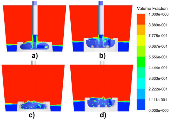
Figure 6.
Volume fractions of gas phase in the two-phase flow during tundish filling operations: (a) TI1, plane passing through the ladle shroud axis; (b) TI3 plane passing through the ladle shroud axis; (c) TI1 plane located at half the distance between the center of the tundish and the wall of the inhibitor; (d) TI3 plane located at half the distance between the center of the tundish and the wall of the inhibitor.
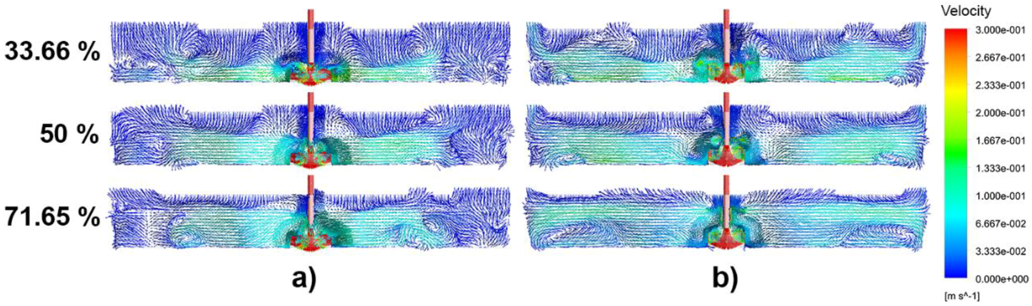
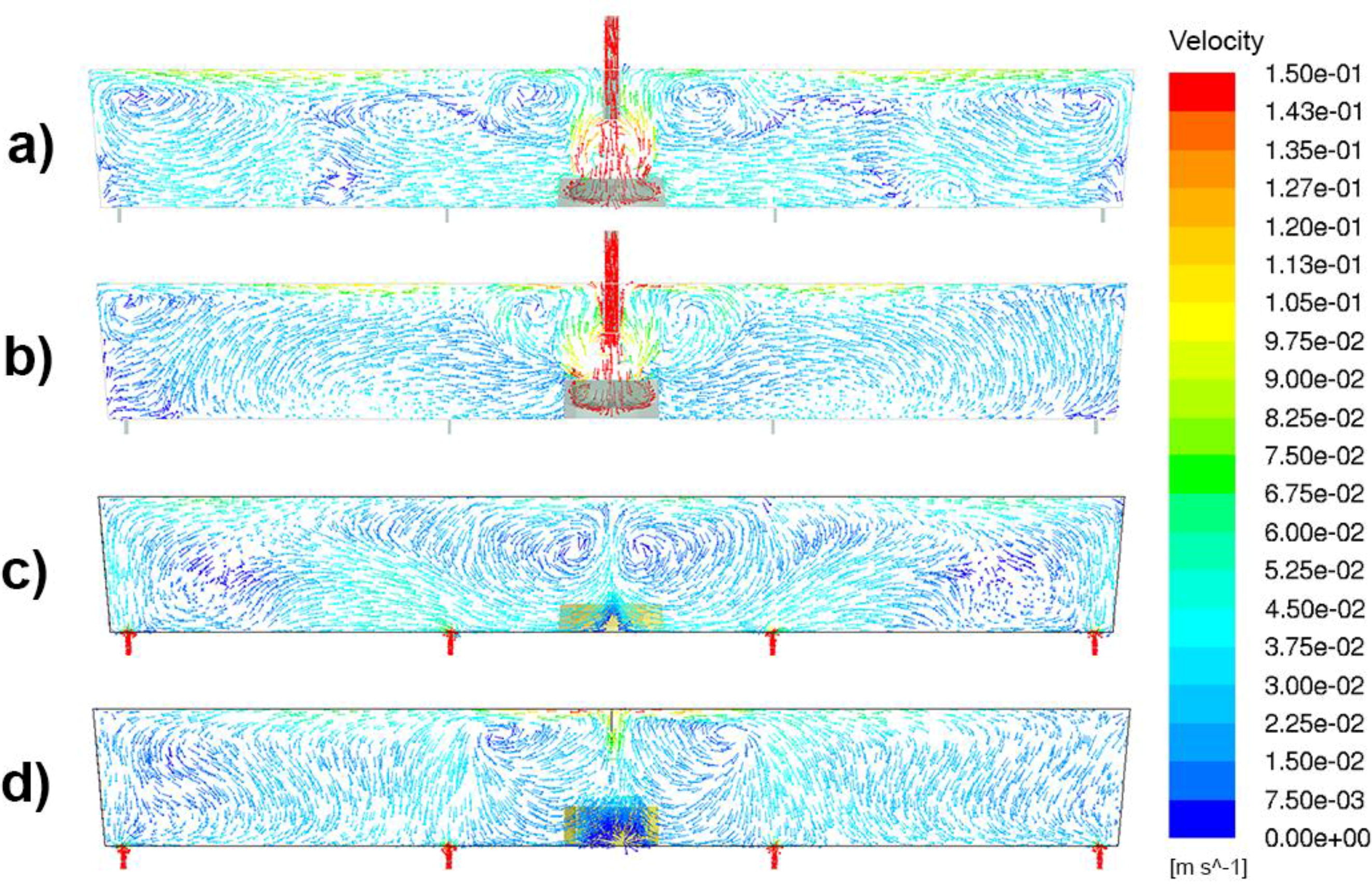
The velocity fields in a longitudinal–vertical plane through the ladle shroud are shown in Figure 7a,b, using TI1 and T13, respectively, at different steel level fillings. At the lowest height percentage recorded in these figures, the liquid lost momentum and impacted the extreme tundish walls with smaller velocities when using TI1 than when using TI3. As the tundish was being filled, this condition remained close to the working level of the tundish. Close to the working level, the lowest flow field (shown in Figure 7b) of the TI3 formed upper long recirculating flows along the tundish while TI1 yielded shorter flows without any apparent defined recirculation (Figure 7a).

Figure 7.
Velocity fields in planes passing through the ladle shroud axis at different height percentages of the operating level in the tundish: (a) TI1; (b) TI3.
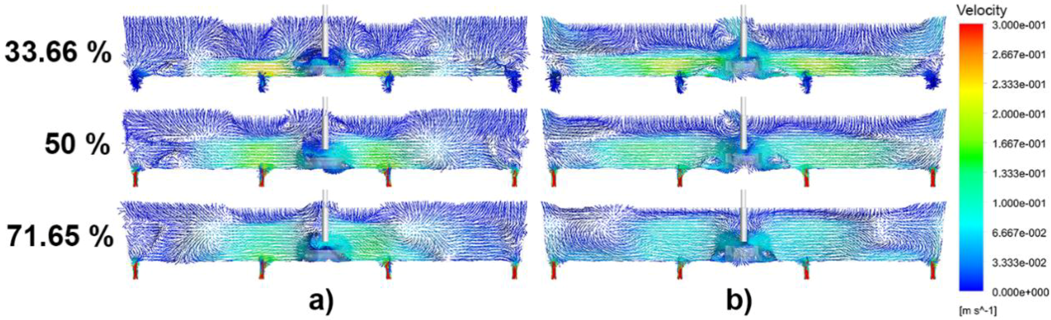
The velocity fields in the same type of plane passing through the strands are presented in Figure 8 at the same bath levels as those shown in the preceding figure (the view of this figure is from the perspective of the delta side of the tundish toward the flat back plane of the tundish, where the ladle shroud is visible because it is in front of the plane where the strands are located, see Figure 2. The first streams of liquid passing through at the lowest height percentage flowed toward the internal strands and, at higher levels, TI3 yielded streams of liquid with relatively high velocities along the tundish bottom while TI1 always yielded streams with lower velocities.
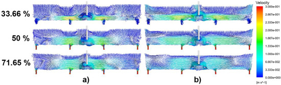
Figure 8.
Velocity fields in planes passing through the positions of the four strands at different height percentages of the operating level in the tundish: (a) TI1; (b) TI3.
The overall effect was that TI1 yielded regions of low velocity in the two extremes of the tundish during the filling operation. This effect could also be seen in horizontal planes, as shown in Figure 9, during the unsteady filling operation for the velocity fields corresponding to the same liquid levels of Figure 7 and Figure 8.
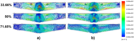
Figure 9.
Velocity fields at different height percentages of the total bath level during operation of the tundish: (a) TI1; (b) TI3.
At any liquid level, TI1 left considerable volumes of liquid with small velocities, while TI3 pushed the liquid, yielding a distributed filling flow. The stability of the gas–liquid interface was maintained during the filling of the tundish, as can be seen by the numerical and experimental results presented in Figure 10 when using either of the two inhibitors. Velocity fields in the vertical planes passing through the axis of the ladle shroud once that the tundish was filled and operating under steady-state conditions are shown in Figure 11a,b using TI1 and TI3, respectively. Figure 11c,d shows the velocity fields in planes passing through the axis of the strands using TI1 and TI3, respectively. TI1 left regions with small velocities mainly in the corner of the tundish.
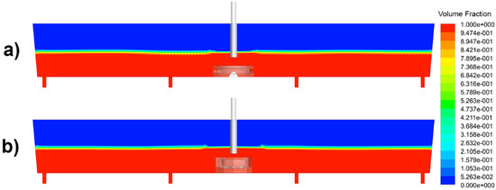
Figure 10.
Stability of the gas–liquid interface during the tundish filling, presented as volume fractions of liquid (red) and gas (blue): (a) TI1; (b) TI3.
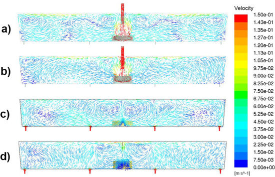
Figure 11.
Velocity fields in vertical planes passing through the axis of the ladle shroud: (a) TI1 and (b) TI3. Velocity fields in planes passing through the four strands: (c) TI1; (d) TI3.
3.3. Experimental and Numerical RTD Curves
A pulse injection of a red dye tracer was injected in the ladle shroud of the water model to determine the RTD curves following the principles explained in chemical engineering textbooks [2,16] under steady-state conditions and full tundish level. These simulations had a twofold purpose: first, to corroborate the predictive capacity of the mathematical model, and second, to demonstrate that even under steady conditions the fluid flow patterns created by each inhibitor during the tundish filling operation prevailed. Therefore, the performance of both inhibitors to control the flow and overall RTD curves were determined using the equations presented in the lower part of Table 2. The outputs of this procedure are reported in the upper part of Table 2, and from these results the following observations were established:
Table 2.
Experimental averaged flow parameters from the residence time distribution (RTD) curves.
- TI2 yielded the highest plug volume fraction (which favors floatation of inclusions), but as mentioned above, delayed the steel stream toward the extreme strands leading to steel freezing problems during startup.
- TI3 yielded a slightly larger plug flow fraction than TI1, with smaller mixed flow fraction.
- The concentration peak of TI3 was the tallest among the three inhibitors.
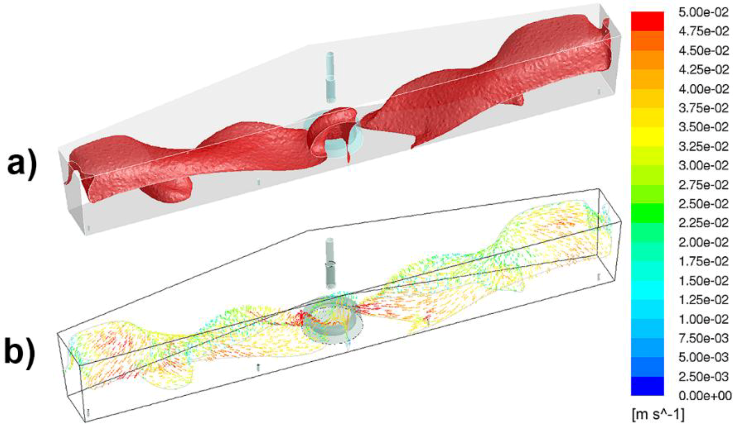
Figure 12a,b shows an isoconcentration surface and the associated velocity field respectively 300 s after the tracer was injected in the ladle shroud for TI1. The liquid transported the tracer close to the tundish bottom after leaving the inhibitor and, as the liquid approached the tundish walls, the tracer was sent toward the surface following the exact velocity field presented in Figure 12b. However, in the same tundish, the TI3 yielded a flow that transported the tracer upwards just after leaving the inhibitor as the isoconcentration surface and the associated velocity field indicated in Figure 13a,b, respectively. In other words, TI3 would eventually send the steel upwards, pushing the inclusions toward the slag phase where they would be absorbed and dissolved.
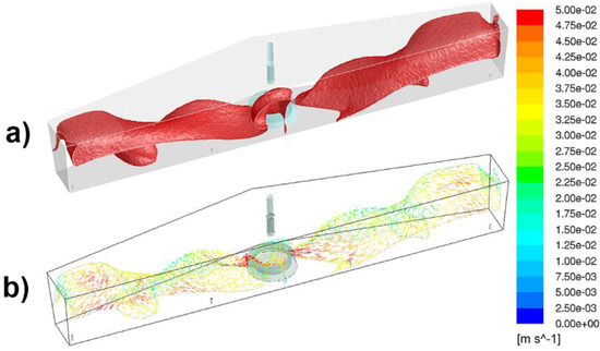
Figure 12.
Tracer mixing kinetics for TI1: (a) Isoconcentration surface in mass fraction of a tracer 300 s after its injection in the ladle shroud and (b) associated velocity field. Isoconcentration surface in mass fraction is 2.6 × 10⁻⁵.
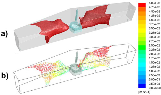
Figure 13.
Tracer mixing kinetics for TI3: (a) Isoconcentration surface in mass fraction of a tracer 300 s after its injection in the ladle shroud and (b) associated velocity field. Isoconcentration surface in mass fraction is 2.6 × 10⁻⁵.
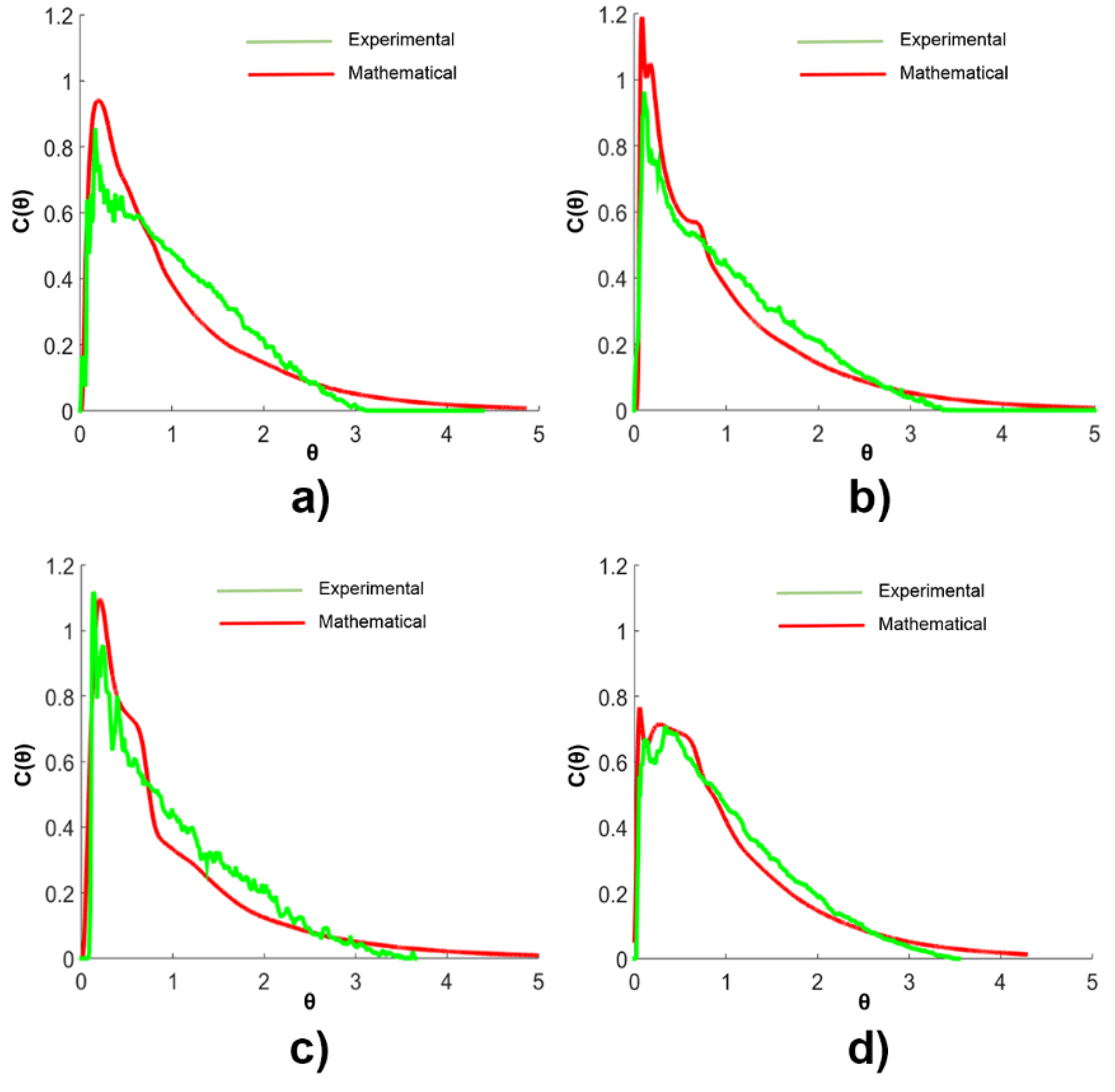
Figure 14a,b shows the individual numerical and calculated RTD curves for the internal and external strands using TI1, and Figure 14c,d shows the individual numerical and calculated RTD curves for the internal and external strands using TI3 curves, respectively. Both numerical and experimental curves match very well, proving that the velocity fields predicted by the mathematical model are reliable and that the model can be used for other tundish designs. The caster is now operating with the inhibitors TI1 and TI3 without any report of steel freezing problems.
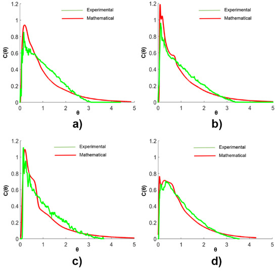
Figure 14.
Experimental and numerical RTD curves: (a) Internal strand, TI1; (b) External strand TI1; (c) Internal strand, TI3; and (d) External strand, TI3.
4. Conclusions
- The coupling of physical and mathematical multiphase simulations provides a powerful modern approach to solve practical industrial problems.
- The VOF model predicts the speed at which the experimental stream of liquid in the tundish flows along the floor very well.
- The current requirements for the optimum design of turbulence inhibitors should include the maximization of plug flow patterns in combination with a good performance during unsteady operations of the tundish.
- The TI3 provides the highest plug flow using a flow pattern that sends the liquid toward the bath surface driving the inclusions toward the metal–slag interface.
Author Contributions
Conceptualization, R.D.M. and K.C.; methodology, R.D.M. and J.G.; software, A.N.-B. and J.R.; validation, J.G., R.D.M. and K.C.; formal analysis, R.D.M. and K.C.; investigation, R.D.M.; resources, K.C.; data curation, R.D.M.; writing—original draft preparation, R.D.M.; writing—review and editing, R.D.M. and K.C.
Acknowledgments
The authors give the thanks to the institutions Consejo Nacional de Ciencia y Tecnologia (CoNaCyT), Sistema Nacional de Investigadores (SNI) and Comision de Fomento de Actividades Acedemicas (COFAA) for their support to this research.
Conflicts of Interest
The authors declare no conflict of interest.
Nomenclature
| C | Concentration of a tracer |
| D0 and Deff | Molecular and turbulent diffusivities |
| F | Additional term force in the Navier–Stokes equations |
| Q | Liquid flow rate through the tundish |
| t | Time |
| tmin | Minimum residence time of the tracer inside the tundish |
| Mean residence time distribution | |
| TI1, TI2, TI3 | Turbulence inhibitors 1, 2, and 3 |
| u, v | Velocities |
| Sc | Schmidt number |
| V | Liquid volume in the tundish |
| Vd, Vdead | Dead volume |
| Vp, VPlug | Plug volume |
| Vm, Vmix. | Mixing volume |
| p | Pressure |
| α | Volume fraction |
| ρ | Density |
| μ | Viscosity |
| λ | Scale factor |
| Phase indicator | |
| θmean | As defined in Table 2. |
| Sub-Indexes | |
| p, q | Phases p and q |
| t | Turbulent |
References
- Morales, R.D.; López-Ramírez, S.; Palafox-Ramos, J.; de Jesus Barreto Sandoval, J.; Zacharias, D. Melt flow control in a multistrand tundish using a turbulence inhibitor. Metall. Mater. Trans. B 2000, 31, 1505–1515. [Google Scholar] [CrossRef]
- Fogler, H.S. Elements of Chemical Reaction Engineering; Prentice Hall Inc.: London, UK, 1992; pp. 708–710. [Google Scholar]
- López-Ramírez, S.; de Jesus Barreto-Sandoval, J.; Morales, R.D.; Zacharias, D. Physical and mathematical determination of the influence of input temperature changes on the molten steel flow characteristics in slab Tundishes. Metall. Mater. Trans. B 2001, 35, 957–966. [Google Scholar] [CrossRef]
- Espino-Zarate, A.; Morales, R.D.; Nájera-Bastida, A.; Macías-Hernández, M.; Sandoval-Ramos, A. Fluid flow and mechanisms of momentum transfer in a six-strand tundish. Metall. Mater. Trans. B 2010, 41, 962–975. [Google Scholar] [CrossRef]
- García-Hernández, S.; Morales, R.D.; de Jesus Barreto Sandoval, J.; Calderón-Ramos, I.; Gutiérrez, E. Modeling study of slag emulsification during ladle change-over using a dissipative ladle shroud. Steel Res. Int. 2016, 87, 1154–1167. [Google Scholar] [CrossRef]
- Morales, R.D.; García-Hernández, S.; de Jesus Barreto Sandoval, J.; Ceballos-Huerta, A.; Ramos, I.C.; Gutiérrez, E. Multiphase flow Modeling of slag entrainment during ladle change-over operation. Metall. Mater. Trans. B 2016, 47, 2595–2606. [Google Scholar] [CrossRef]
- Morales, R.D.; Guarneros, J.; Nájera-Bastida, A.; Rodrñiguez, J. Control of two-phase flows during startup operations of casting sequences in a billet tundish. JOM 2018, 70, 2103–2108. [Google Scholar] [CrossRef]
- Frank, M. White, Fluid Mechanics, 4th ed.; McGraw-Hill: New York, NY, USA, 1999; pp. 294–296. [Google Scholar]
- Hirth, C.W.; Nichols, B.D. Volume of Fluid (VOF) Method for the Dynamics of Free Boundaries. J. Comput. Phys. 1981, 39, 201. [Google Scholar] [CrossRef]
- Yeoh, G.H.; Tu, J. Computational Techniques for Multiphase Flows; Butterworth-Heinemann: Oxford, UK, 2010; pp. 133–170. [Google Scholar]
- Manual of ANSYS-FLUENT. Available online: http://www.ansys.com/Products/Fluids/ANSYS-Fluent (accessed on 5 March 2018).
- Ferziger, H.; Peric, M. Computational Methods for Fluid Dynamics; Springer: New York, NY, USA; Berlin, Germany, 2002; pp. 72–75. [Google Scholar]
- Bird, R.B.; Stewart, W.E.; Lightfoot, E.N. Transport. Phenomena, 2nd ed.; John Wiley & Sons: New York, NY, USA, 2007; pp. 166–168. [Google Scholar]
- Brackbill, J.U.; Kothe, D.B.; Zemack, C. A continuum method for modeling surface tension. J. Comput. Phys. 1992, 100, 335–354. [Google Scholar] [CrossRef]
- Manual of Solid Works. Available online: www.solidworks.com (accessed on 5 March 2018).
- Levenspiel, O. Chemical Reaction Engineering; John Wiley and Sons: New York, NY, USA, 1999; pp. 257–312. [Google Scholar]


© 2019 by the authors. Licensee MDPI, Basel, Switzerland. This article is an open access article distributed under the terms and conditions of the Creative Commons Attribution (CC BY) license (http://creativecommons.org/licenses/by/4.0/).