Modeling of Ti6Al4V Alloy Orthogonal Cutting with Smooth Particle Hydrodynamics: A Parametric Analysis on Formulation and Particle Density


Abstract
1. Introduction
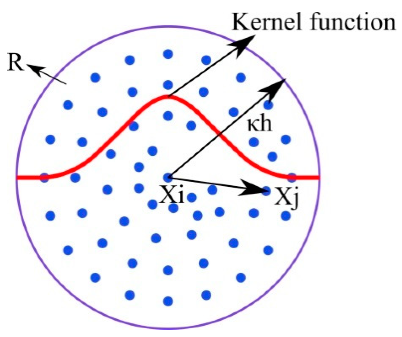
2. SPH Foundations
3. Material Modeling
3.1. Constitutive Model
3.2. Equation of State
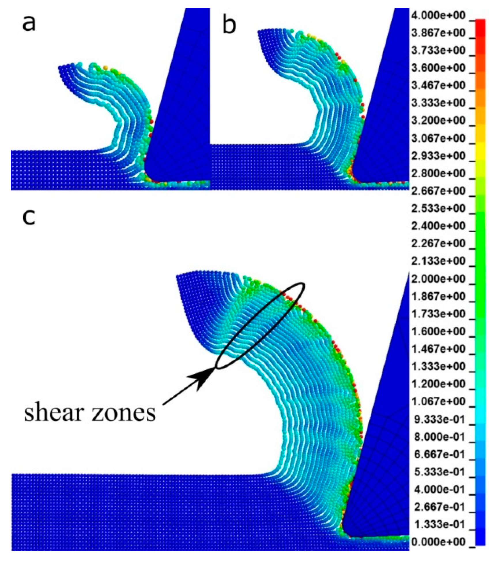
3.3. Material Separation Modelling
3.4. Contact and Friction Modeling
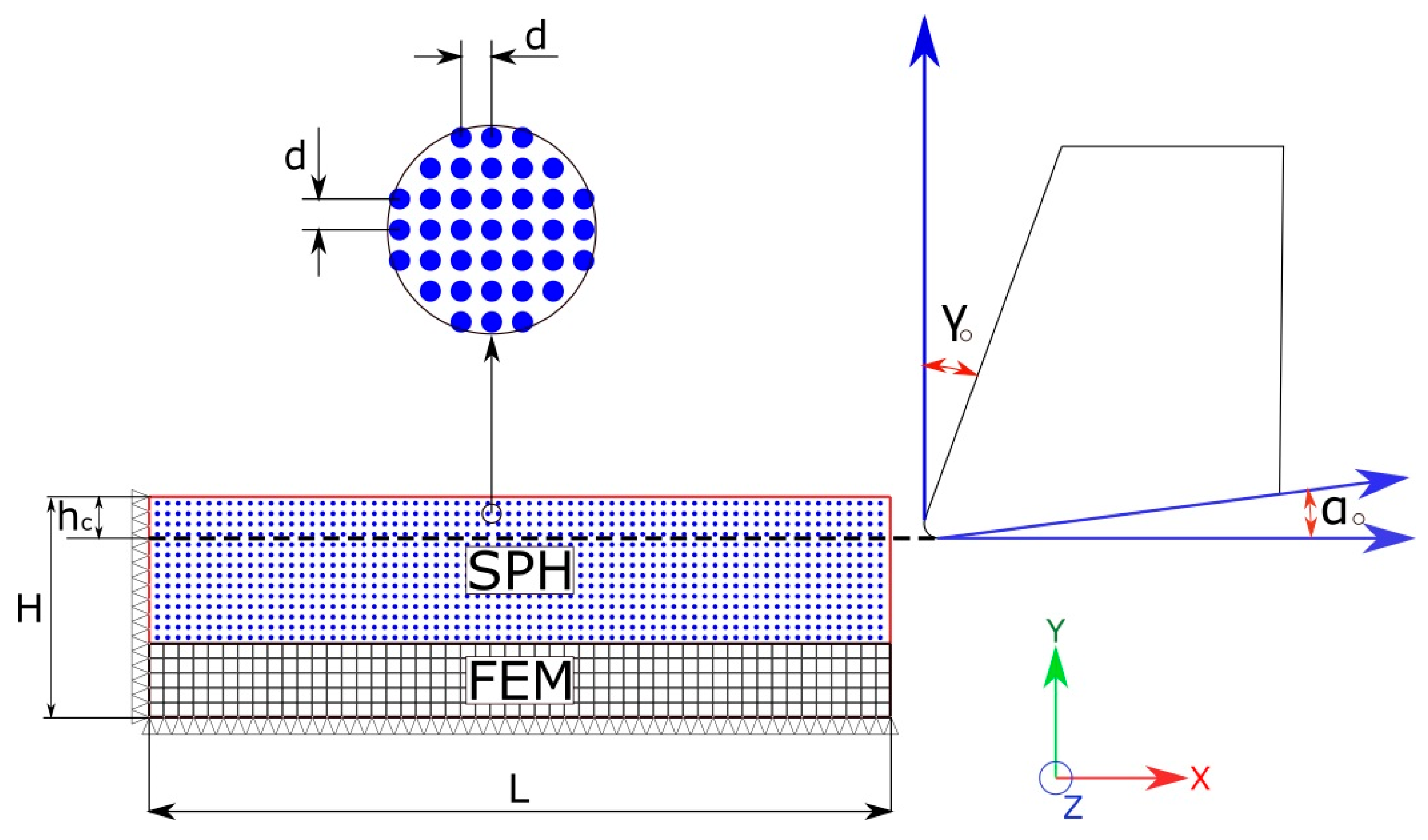
4. Numerical Simulation Configuration
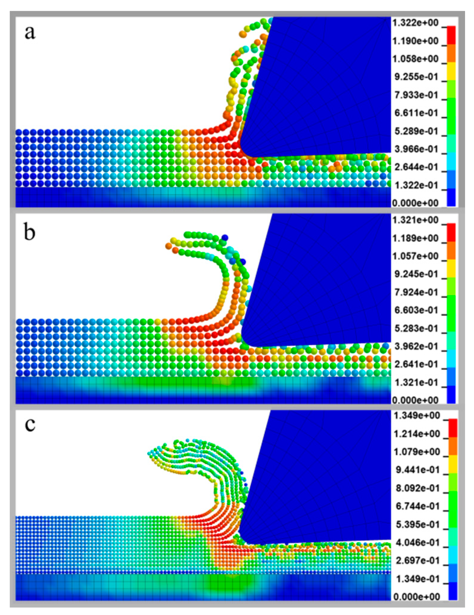
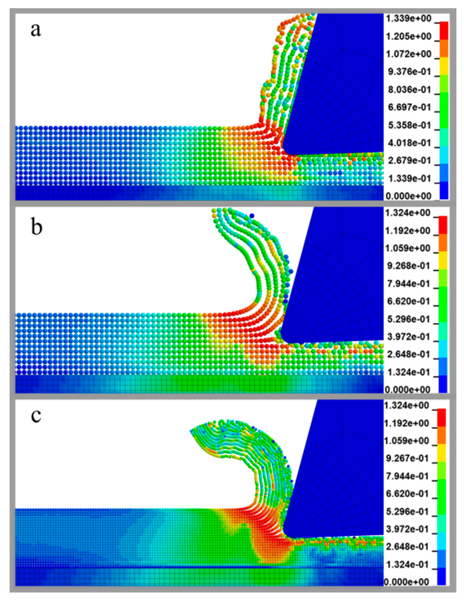
5. Results and Discussion
6. Conclusions
Author Contributions
Funding
Conflicts of Interest
Nomenclature
| A | Initial yield stress [MPa] |
| B | Hardening constant [MPa] |
| C | Strain Rate Constant |
| d | Distance between particles [mm] |
| E | Young’s Modulus [GPa] |
| Cutting Force [N/mm] | |
| Feed Force [N/mm] | |
| f | Friction coefficient |
| H | Height of the workpiece [mm] |
| h | Smoothing length [mm] |
| hc | Depth of cut [mm] |
| K | Bulk modulus [GPa] |
| L | Length of the workpiece [mm] |
| m | Thermal softening exponent |
| Mass of particle | |
| n | Hardening exponent |
| P | Pressure [GPa] |
| r | Cutting edge radius [μm] |
| Room temperature [K] | |
| Melting temperature [K] | |
| V | Cutting speed [m/s] |
| Wc | Width of the workpiece |
| W | Kernel function |
| Position vector of particle i | |
| x | Position vector of a point in space |
| α | Clearance angle [deg] |
| γ | Rake angle [deg] |
| Dirac function | |
| Volume of particle | |
| Equivalent strain | |
| Equivalent strain rate [1/s] | |
| Reference strain rate [1/s] | |
| Relative change of density | |
| ρ | Density [] |
| Density of particle | |
| Normal stress [GPa] | |
| Equivalent stress [GPa] | |
| Frictional stress [GPa] |
References
- Welsch, G.; Boyer, R.; Collings, E.W. (Eds.) Materials Properties Handbook: Titanium Alloys; ASM International: Materials Park, OH, USA, 1994; ISBN 978-0-87170-481-8. [Google Scholar]
- Davim, J.P. (Ed.) Machining of Titanium Alloys; Springer: New York, NY, USA, 2014; ISBN 978-3-662-43901-2. [Google Scholar]
- Ezugwu, E.O.; Wang, Z.M. Titanium alloys and their machinability—A review. J. Mater. Process. Technol. 1997, 68, 262–274. [Google Scholar] [CrossRef]
- Mamalis, A.G.; Horváth, M.; Branis, A.S.; Manolakos, D.E. Finite element simulation of chip formation in orthogonal metal cutting. J. Mater. Process. Technol. 2001, 110, 19–27. [Google Scholar] [CrossRef]
- Ng, E.-G.; Aspinwall, D.K. Modelling of hard part machining. J. Mater. Process. Technol. 2002, 127, 222–229. [Google Scholar] [CrossRef]
- Guo, Y.B.; Yen, D.W. A FEM study on mechanisms of discontinuous chip formation in hard machining. J. Mater. Process. Technol. 2004, 155–156, 1350–1356. [Google Scholar] [CrossRef]
- Hua, J.; Shivpuri, R. Prediction of chip morphology and segmentation during the machining of titanium alloys. J. Mater. Process. Technol. 2004, 150, 124–133. [Google Scholar] [CrossRef]
- Rhim, S.-H.; Oh, S.-I. Prediction of serrated chip formation in metal cutting process with new flow stress model for AISI 1045 steel. J. Mater. Process. Technol. 2006, 171, 417–422. [Google Scholar] [CrossRef]
- Calamaz, M.; Coupard, D.; Girot, F. A new material model for 2D numerical simulation of serrated chip formation when machining titanium alloy Ti–6Al–4V. Int. J. Mach. Tools Manuf. 2008, 48, 275–288. [Google Scholar] [CrossRef]
- Sima, M.; Özel, T. Modified material constitutive models for serrated chip formation simulations and experimental validation in machining of titanium alloy Ti–6Al–4V. Int. J. Mach. Tools Manuf. 2010, 50, 943–960. [Google Scholar] [CrossRef]
- Pimenov, D.Y.; Guzeev, V.I.; Koshin, A.A. Influence of cutting conditions on the stress at tool’s rear surface. Russ. Eng. Res. 2011, 31, 1151–1155. [Google Scholar] [CrossRef]
- Pimenov, D.Y.; Guzeev, V.I. Mathematical model of plowing forces to account for flank wear using FME modeling for orthogonal cutting scheme. Int. J. Adv. Manuf. Technol. 2017, 89, 3149–3159. [Google Scholar] [CrossRef]
- Ducobu, F.; Rivière-Lorphèvre, E.; Filippi, E. Influence of the Material Behavior Law and Damage Value on the Results of an Orthogonal Cutting Finite Element Model of Ti6Al4V. In Proceedings of the 14th CIRP Conference on Modeling of Machining Operations (CIRP CMMO), Turin, Italy, 13–14 June 2013; Settineri, L., Ed.; Elsevier: Amsterdam, The Netherlands, 2013; pp. 379–384. [Google Scholar]
- Boldyrev, I.S.; Shchurov, I.A.; Nikonov, A.V. Numerical Simulation of the Aluminum 6061-T6 Cutting and the Effect of the Constitutive Material Model and Failure Criteria on Cutting Forces’ Prediction. In Proceedings of the 2nd International Conference on Industrial Engineering (ICIE-2016), Chelyabinsk, Russia, 19–20 May 2016; Radionov, A.A., Ed.; Elsevier: Amsterdam, The Netherlands, 2016; pp. 866–870. [Google Scholar]
- Ducobu, F.; Arrazola, P.-J.; Rivière-Lorphèvre, E.; de Zarate, G.O.; Madariaga, A.; Filippi, E. The CEL Method as an Alternative to the Current Modelling Approaches for Ti6Al4V Orthogonal Cutting Simulation. In Proceedings of the 16th CIRP Conference on Modelling of Machining Operations (16th CIRP CMMO), Cluny, France, 15–16 June 2017; Outeiro, J., Poulachon, G., Eds.; Elsevier: Amsterdam, The Netherlands, 2017; pp. 245–250. [Google Scholar]
- Ducobu, F.; Rivière-Lorphèvre, E.; Filippi, E. Finite element modelling of 3D orthogonal cutting experimental tests with the Coupled Eulerian-Lagrangian (CEL) formulation. Finite Elem. Anal. Des. 2017, 134, 27–40. [Google Scholar] [CrossRef]
- Grissa, R.; Zemzemi, F.; Fathallah, R. Three approaches for modeling residual stresses induced by orthogonal cutting of AISI316L. Int. J. Mech. Sci. 2018, 135, 253–260. [Google Scholar] [CrossRef]
- Gingold, R.A.; Monaghan, J.J. Smoothed particle hydrodynamics: theory and application to non-spherical stars. Mon. Not. R. Astron. Soc. 1977, 181, 375–389. [Google Scholar] [CrossRef]
- Libersky, L.D.; Petschek, A.G. Smooth particle hydrodynamics with strength of materials. In Advances in the Free-Lagrange Method Including Contributions on Adaptive Gridding and the Smooth Particle Hydrodynamics Method; Trease, H.E., Fritts, M.F., Crowley, W.P., Eds.; Springer: Berlin, Germany, 1991; Volume 395, pp. 248–257. ISBN 978-3-540-54960-4. [Google Scholar]
- Liu, G.R. Meshfree Methods: Moving Beyond the Finite Element Method, 2nd ed.; CRC Press: Boca Raton, FL, USA, 2009; ISBN 978-1-4200-8210-4. [Google Scholar]
- Liu, G.R.; Liu, M.B. Smoothed Particle Hydrodynamics: A Meshfree Particle Method; World Scientific: Hackensack, NJ, USA, 2003; ISBN 978-981-238-456-0. [Google Scholar]
- Heinstein, M.; Segalman, D. Simulation of Orthogonal Cutting with Smooth Particle Hydrodynamics; SAND-97-1961; Sandia National Labs.: Albuquerque, NM, USA, 1 September 1997.
- Limido, J.; Espinosa, C.; Salaün, M.; Lacome, J.L. SPH method applied to high speed cutting modelling. Int. J. Mech. Sci. 2007, 49, 898–908. [Google Scholar] [CrossRef]
- Calamaz, M.; Limido, J.; Nouari, M.; Espinosa, C.; Coupard, D.; Salaün, M.; Girot, F.; Chieragatti, R. Toward a better understanding of tool wear effect through a comparison between experiments and SPH numerical modelling of machining hard materials. Int. J. Refract. Met. Hard Mater. 2009, 27, 595–604. [Google Scholar] [CrossRef]
- Villumsen, M.F.; Fauerholdt, T.G. Simulation of Metal Cutting using Smooth Particle Hydrodynamics. In Proceedings of the 7th LS-DYNA Anwenderforum, Bamberg, Germany, 30 September–1 October 2008; pp. 17–36. [Google Scholar]
- Bagci, E. 3-D numerical analysis of orthogonal cutting process via mesh-free method. Int. J. Phys. Sci. 2011, 6, 1267–1282. [Google Scholar]
- Dănuț, J. SPH Meshless Simulation of Orthogonal Cutting of AA6060-T6. Appl. Mech. Mater. 2015, 808, 258–263. [Google Scholar] [CrossRef]
- Spreng, F.; Eberhard, P. Machining Process Simulations with Smoothed Particle Hydrodynamics. In Proceedings of the 15th CIRP Conference on Modelling of Machining Operations, Karlsruhe, Germany, 11–12 June 2015; pp. 94–99. [Google Scholar]
- Umer, U.; Mohammed, M.K.; Qudeiri, J.A.; Al-Ahmari, A. Assessment of finite element and smoothed particles hydrodynamics methods for modeling serrated chip formation in hardened steel. Adv. Mech. Eng. 2016, 8, 1–11. [Google Scholar] [CrossRef]
- Geng, X.; Dou, W.; Deng, J.; Yue, Z. Simulation of the cutting sequence of AISI 316L steel based on the smoothed particle hydrodynamics method. Int. J. Adv. Manuf. Technol. 2017, 89, 643–650. [Google Scholar] [CrossRef]
- Madaj, M.; Píška, M. On the SPH Orthogonal Cutting Simulation of A2024-T351 Alloy. In Proceedings of the 14th CIRP Conference on Modeling of Machining Operations, Turin, Italy, 13–14 June 2013; Settineri, L., Ed.; Elsevier: Amsterdam, The Netherlands, 2013; pp. 152–157. [Google Scholar]
- Olleak, A.A.; El-Hofy, H.A. SPH Modelling of Cutting Forces while Turning of Ti6Al4V Alloy. In Proceedings of the 10th European LS-DYNA Conference, Würzburg, Germany, 15–17 June 2015. [Google Scholar]
- Takabi, B.; Tajdari, M.; Tai, B.L. Numerical study of smoothed particle hydrodynamics method in orthogonal cutting simulations – effects of damage criteria and particle density. J. Manuf. Process. 2017, 30, 523–531. [Google Scholar] [CrossRef]
- Heisel, U.; Zaloga, W.; Krivoruchko, D.; Storchak, M.; Goloborodko, L. Modelling of orthogonal cutting processes with the method of smoothed particle hydrodynamics. Prod. Eng. 2013, 7, 639–645. [Google Scholar] [CrossRef]
- Avachat, C.S.; Cherukuri, H.P. A Parametric Study of the Modeling of Orthogonal Machining Using the Smoothed Particle Hydrodynamics Method. In Proceedings of the ASME 2015 International Mechanical Engineering Congress and Exposition, Houston, TX, USA, 13–19 November 2015; ASME: Houston, TX, USA, 2015; p. V014T06A005. [Google Scholar]
- Limido, J.; Espinosa, C.; Salaun, M.; Mabru, C.; Chieragatti, R.; Lacome, J.L. Metal cutting modelling SPH approach. Int. J. Mach. Mach. Mater. 2011, 9, 177–196. [Google Scholar] [CrossRef]
- Randles, P.W.; Libersky, L.D. Smoothed Particle Hydrodynamics: Some recent improvements and applications. Comput. Methods Appl. Mech. Eng. 1996, 139, 375–408. [Google Scholar] [CrossRef]
- Vila, J.P. SPH Renormalized Hybrid Methods for Conservation Laws: Applications to Free Surface Flows. In Meshfree Methods for Partial Differential Equations II; Griebel, M., Schweitzer, M.A., Eds.; Springer: Berlin, Germany, 2005; Volume 43, pp. 207–229. ISBN 978-3-540-23026-7. [Google Scholar]
- Livermore Software Technology Corporation. LS-DYNA KEYWORD USER’S MANUAL; Livermore Software Technology Corporation: Livermore, CA, USA, 2017. [Google Scholar]
- Monaghan, J.J.; Lattanzio, J.C. A refined particle method for astrophysical problems. Astron. Astrophys. 1985, 149, 135–143. [Google Scholar]
- Seo, S.; Min, O.; Yang, H. Constitutive equation for Ti–6Al–4V at high temperatures measured using the SHPB technique. Int. J. Impact Eng. 2005, 31, 735–754. [Google Scholar] [CrossRef]
- Ducobu, F.; Rivière-Lorphèvre, E.; Filippi, E. On the importance of the choice of the parameters of the Johnson-Cook constitutive model and their influence on the results of a Ti6Al4V orthogonal cutting model. Int. J. Mech. Sci. 2017, 122, 143–155. [Google Scholar] [CrossRef]
- Ducobu, F.; Rivière-Lorphèvre, E.; Filippi, E. Experimental contribution to the study of the Ti6Al4V chip formation in orthogonal cutting on a milling machine. Int. J. Mater. Form. 2015, 8, 455–468. [Google Scholar] [CrossRef]


| Material Parameters | Values |
|---|---|
| A (MPa) | 997.9 |
| B (MPa) | 653.1 |
| C | 0.0198 |
| m | 0.7 |
| n | 0.45 |
| (s−1) | 1 |
| (K) | 298 |
| (K) | 1878 |
| Young’s Modulus (E, GPa) | 113.8 |
| Density ρ ( | 4430 |
| Friction coefficient (f) | 0.2 |
| Al | C | Fe | H | N | O | V | OT |
|---|---|---|---|---|---|---|---|
| 5.5–6.75 | 0.1 | 0.3 | 0.0125 | 0.05 | 0.2 | 3.5–4.5 | 0.4 |
| Machining Parameters | Values | ||
|---|---|---|---|
| Cutting speed V [m/s] | 0.5 | ||
| Rake angle, γ [deg] | 15 | ||
| Clearance angle, α [deg] | 2 | ||
| Cutting edge radius r [μm] | 20 | ||
| Depth of cut, hc [mm] | 0.04 | 0.06 | 0.1 |
| Depth of Cut hc [mm] | Experimental Cutting Force [N/mm] | Standard Formulation (d = 0.01 [mm]) [N/mm] | Renormalized Formulation (d = 0.01 [mm]) [N/mm] | Renormalized Formulation (d = 0.005 [mm]) [N/mm] |
|---|---|---|---|---|
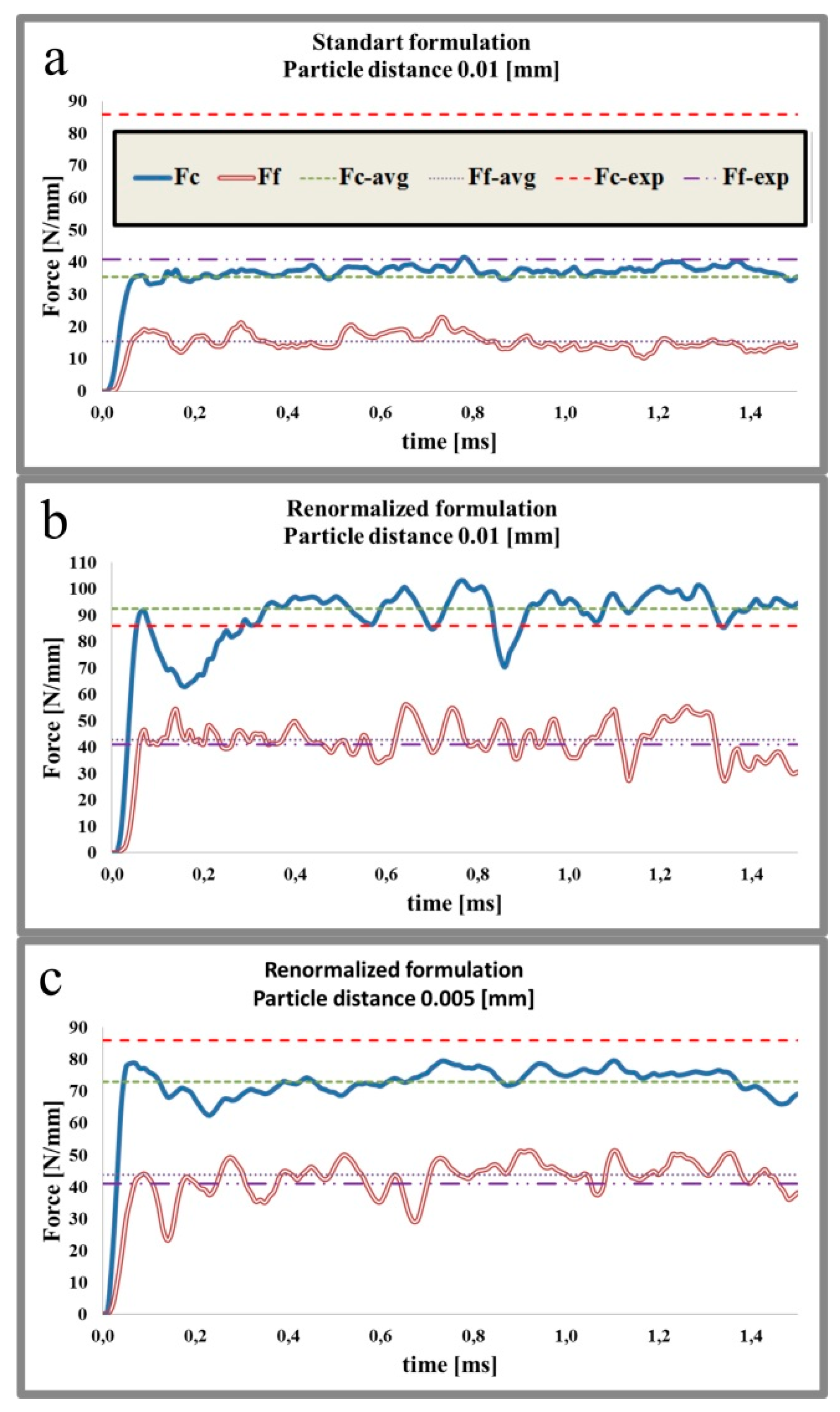
| 0.04 | 86 | 35.6 | 92.5 | 73 |
| −58.6% | +7.6% | −15.1% | ||
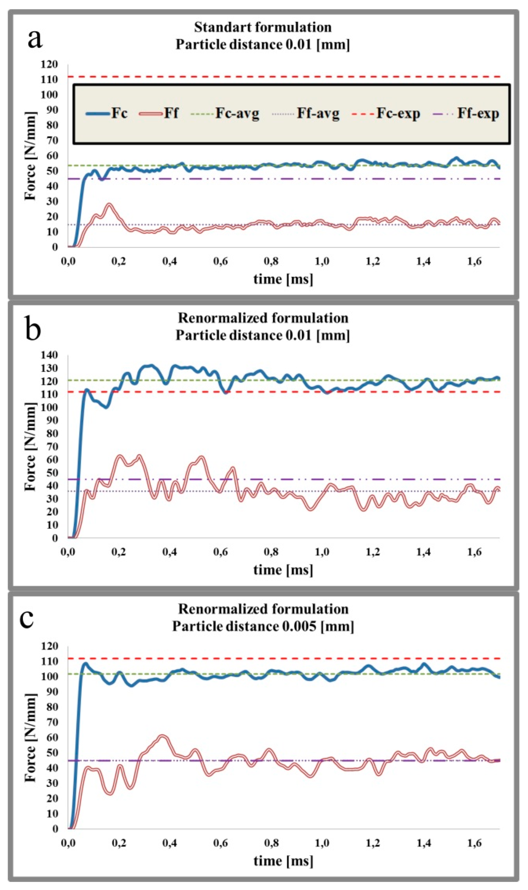
| 0.06 | 112 | 53,76 | 120.9 | 101.9 |
| −52% | +7.94% | −9.02% | ||
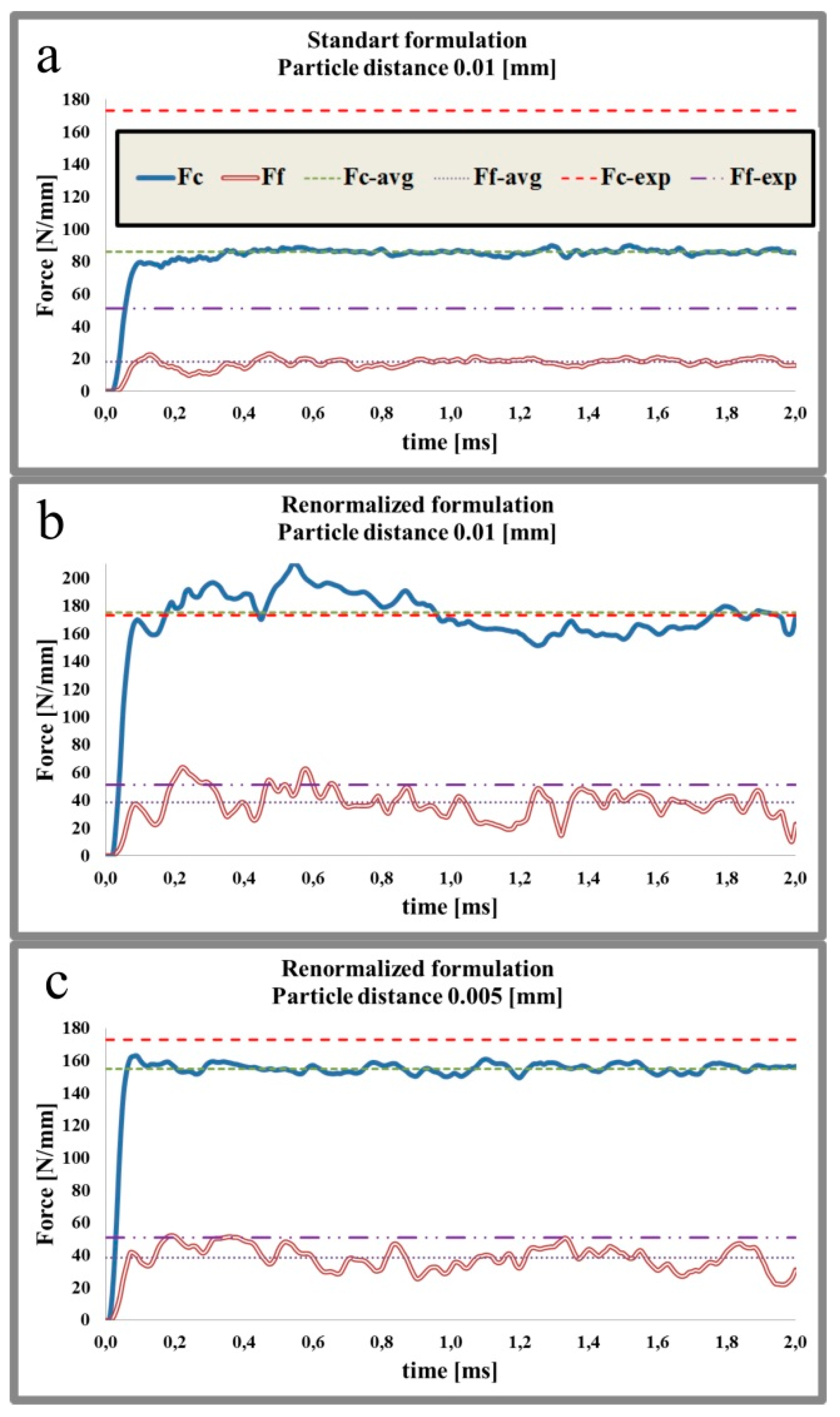
| 0.1 | 173 | 86 | 175 | 155 |
| −50.3% | +1.2% | −10.4% |
| Depth of Cut hc [mm] | Experimental Feed Force [N/mm] | Standard Formulation (d = 0.01 [mm]) [N/mm] | Renormalized Formulation (d = 0.01 [mm]) [N/mm] | Renormalized Formulation (d = 0.005 [mm]) [N/mm] |
|---|---|---|---|---|
| 0.04 | 41 | 15.5 | 42.8 | 43.8 |
| −62,2% | +4.39% | +6.8% | ||
| 0.06 | 45 | 14.9 | 35.95 | 45.1 |
| −66,9% | −20.1% | 0.2% | ||
| 0.1 | 51 | 18.15 | 38.39 | 38.6 |
| −64.4% | −24.7% | −24.3% |
© 2019 by the authors. Licensee MDPI, Basel, Switzerland. This article is an open access article distributed under the terms and conditions of the Creative Commons Attribution (CC BY) license (http://creativecommons.org/licenses/by/4.0/).
Share and Cite
Lampropoulos, A.D.; Markopoulos, A.P.; Manolakos, D.E. Modeling of Ti6Al4V Alloy Orthogonal Cutting with Smooth Particle Hydrodynamics: A Parametric Analysis on Formulation and Particle Density. Metals 2019, 9, 388. https://doi.org/10.3390/met9040388
Lampropoulos AD, Markopoulos AP, Manolakos DE. Modeling of Ti6Al4V Alloy Orthogonal Cutting with Smooth Particle Hydrodynamics: A Parametric Analysis on Formulation and Particle Density. Metals. 2019; 9(4):388. https://doi.org/10.3390/met9040388
Chicago/Turabian StyleLampropoulos, Adam D., Angelos P. Markopoulos, and Dimitrios E. Manolakos. 2019. "Modeling of Ti6Al4V Alloy Orthogonal Cutting with Smooth Particle Hydrodynamics: A Parametric Analysis on Formulation and Particle Density" Metals 9, no. 4: 388. https://doi.org/10.3390/met9040388
APA StyleLampropoulos, A. D., Markopoulos, A. P., & Manolakos, D. E. (2019). Modeling of Ti6Al4V Alloy Orthogonal Cutting with Smooth Particle Hydrodynamics: A Parametric Analysis on Formulation and Particle Density. Metals, 9(4), 388. https://doi.org/10.3390/met9040388