On the Design of Innovative Heterogeneous Sheet Metal Tests Using a Shape Optimization Approach ^†

Abstract

The development of full-field measurement methods has enabled a new trend of heterogeneous mechanical tests. The inhomogeneous strain fields retrieved from these tests are being widely used in the calibration of constitutive models for sheet metals. However, today, there is no mechanical test able to characterize the material in a large range of strain states. The aim of this work is to present a heterogeneous mechanical test with an innovative tool/specimen shape, capable of producing rich heterogeneous strain paths and thus providing extensive information on material behavior. The proposed specimen is found using a shape optimization process where an index that evaluates the richness of strain information is used. In this work, the methodology and results are extended to non-specimen geometry dependence and to the non-dependence of the geometry parametrization through the use of the Ritz method for boundary value problems. Different curve models, such as splines, B-splines, and NURBS, are used, and C1 continuity throughout the specimen is guaranteed. Moreover, several deterministic and stochastic optimization methods are used in order to find the method or the combination of methods able to minimize the cost function effectively. Results demonstrated that the solution is dependent on the geometry definition, as well as on the optimization methodology. Nevertheless, the obtained solutions provided a wider spectrum of strain states than standard tests.

1. Introduction

Industry is increasingly demanding and becoming more competitive. Due to efficiency and cost reduction requirements, numerical simulation has been applied to sheet metal-forming processes since the 1960s [1]. Currently, numerical simulations can accurately replicate the forming process due to the ability to process complex iterative calculus using material properties, surface properties, and process conditions [2]. However, to this end, the finite element models must have accurate constitutive models and well-defined material parameters. Due to the rolling process, sheet metals exhibit orthotropic behavior. This anisotropy influences the sheet metal-forming operations’ results, implying the use of complex constitutive mathematical models capable of describing the material behavior [3,4].

Constitutive models consist of functions that accurately describe the material behavior. The complexity of these models determines the number of material parameters to identify. Usually, Finite Element Modeling Update (FEMU) or equilibrium techniques are used to determine the models’ input data. FEMU consists of an iterative inverse technique that begins with a known solution and identifies the constitutive parameters minimizing the difference between known and predicted forces and/or displacement fields [5]. However, methods based on equilibrium satisfaction, such as the Virtual Field Method (VFM) or the Equilibrium Gap Method (EGM), search for the parameters that satisfy equilibrium equations (in the local or weak form) using a known (experimental) kinematic field (displacement or strain).

Regardless of the method, the parameter identification depends on the amount and quality of experimental data. There are two approaches related to experimental data: homogeneous and non-homogeneous tests [4]. The first approach uses classical tests, i.e., tensile test, shear test, etc. Each test usually produces homogeneous strain fields that allow identifying a limited number of parameters, requiring a large number of tests to identify the constitutive parameters properly [6]. The second approach is related to Full-Field Measurement (FFM) strategies. Due to the development of FFM methods and Digital Image Correlation (DIC), it is possible to obtain the strain or displacement field data on the surface of the specimen. Theoretically, with this extensive amount of information, it should be possible to identify a large set of parameters using only one test. This leads to a reduction of the experimental test set used to build the experimental database [7,8]. As a result of these innovative techniques, this field of research has been growing. Some proposals for non-standard uniaxial tests [9] and also for non-standard biaxial tensile specimens [10] have already been published. In the published works, the specimens used can have different cross-sections and geometries (holes, cuts, etc.), promoting heterogeneous displacement fields through the specimen. Moreover, some original tests introduced new designs, such as the geometry presented by Pottier [11]. A review of the mechanical tests commonly used for parameter identification can be seen in [12,13]. However, none of the presented tests can promote a very wide spectrum of strain states with a large magnitude of plastic strain.

The main goal of this work is to design a tool-specimen capable of maximizing the number of heterogeneous strain states, as well as plastic strain range. To this end, a numerical iterative process that optimizes the test geometry is used. In each iteration, an indicator capable of quantifying and rating the mechanical information provided by the test is used. Although this approach is completely numerical, recent works [14] experimentally validated this design by an optimization methodology. The approach used is similar to the ones used in recent works [4,7,15]. However, previous works have only considered a constant number of design variables without analyzing the influence of the number of variables in the solution. Additionally, it is known [15,16] that the curve model that defines the geometry, such as splines, B-splines, or NURBS, influences the shape optimization process. Moreover, design processes are initial solution dependent when using gradient-based or the direct search optimization algorithm, such as the ones used in the mentioned previous works.

This work focuses on analyzing and solving some of the mentioned limitations of the previous works. Therefore, in this work, a Ritz-type design methodology is used to minimize the dependence of the geometry definition model, as well as the number of design control points. Additionally, several optimization algorithms are used, including a global search and a metaheuristic algorithm, to avoid initial solution dependence and analyze the performance of the design-by-optimization process.

2. Methodology

2.1. Constitutive Model

An appropriate constitutive model is a prerequisite for accurate simulations and design. In this work, a phenomenological model composed by the non-quadratic Yld2004-18p yield criterion combined with a mixed isotropic-kinematic hardening law is used. Additionally, the rupture behavior of DC04 is characterized by the calibration of the macroscopic Cockcroft and Latham (CL) rupture criterion [15].

Table 1. Constitutive equations that describe the mechanical behavior of the material. Data from [4].

Isotropic hardening:

${\sigma }_{\mathrm{Y}}\left({\overline{\epsilon }}^{\mathrm{P}}\right)={\sigma }_0+({\sigma }_{\infty }-{\sigma }_0)[1-\exp (-\delta {\overline{\epsilon }}^{\mathrm{P}})]+\beta {\overline{\epsilon }}^{\mathrm{P}}$

Kinematic hardening:

$\dot{\mathit{\alpha }}={\sum }_{i=1}^3\dot{\mathit{\alpha }}={\sum }_{i=1}^3\left(\frac{C_i}{\overline{\eta }}\mathit{\eta }-{\gamma }_i·{\mathit{\alpha }}_i\right){\dot{\overline{\epsilon }}}^{\mathrm{p}}$

Yld2004-18p yield criterion:

$\overline{\eta }{\left(\mathit{\eta }\right)}^a={\sum }_{i=1,j=1}^3{\left|{\tilde{\mathbf{S}}}_i^1-{\tilde{\mathbf{S}}}_j^2\right|}^{\mathrm{a}}=4{\sigma }_{\mathrm{Y}}^a$

${\tilde{\mathbf{S}}}^{\left(k\right)}={\tilde{\mathbf{L}}}^{\left(k\right)}:\mathbf{S},k=1,2$

${\tilde{\mathbf{L}}}^{\left(k\right)}=\left[\begin{array}{cccccc}0& -c_{12}^{\left(k\right)}& -c_{13}^{\left(k\right)}& 0& 0& 0\\ -c_{21}^{\left(k\right)}& 0& -c_{23}^{\left(k\right)}& 0& 0& 0\\ -c_{31}^{\left(k\right)}& -c_{32}^{\left(k\right)}& 0& 0& 0& 0\\ 0& 0& 0& -c_{44}^{\left(k\right)}& 0& 0\\ 0& 0& 0& 0& -c_{55}^{\left(k\right)}& 0\\ 0& 0& 0& 0& 0& -c_{66}^{\left(k\right)}\end{array}\right]$

Rupture criterion:

$W={\int }_0^{{\overline{\epsilon }}_{\mathrm{P}}^{\mathrm{f}}}\frac{{\sigma }_I}{\overline{\eta }}\mathrm{d}{\overline{\epsilon }}^{\mathrm{P}}\le W_{\mathrm{CL}}^{\mathrm{f}}$

sums up the constitutive equations that describe the material behavior. A detailed description of the model and a parameter identification procedure for a DC04 mild steel can be found in previous works [4,17]. The values of isotropic and kinematic hardening coefficients used in this work, as well as the Yld2004-18p yield anisotropy coefficients are listed in

Table 2. Constitutive model parameters used in this work. Data from [17].

Parameter	Value	Units	Parameter	Value	Units
$c_{12}^{\left(1\right)}$	1.264	-	$c_{13}^{\left(1\right)}$	0.974	-
$c_{21}^{\left(1\right)}$	1.242	-	$c_{23}^{\left(1\right)}$	1.049	-
$c_{31}^{\left(1\right)}$	0.578	-	$c_{32}^{\left(1\right)}$	0.708	-
$c_{44}^{\left(1\right)}=c_{55}^{\left(1\right)}$	1.000	-	$c_{66}^{\left(1\right)}$	1.365	-
$c_{12}^{\left(2\right)}$	0.793	-	$c_{13}^{\left(2\right)}$	0.672	-
$c_{21}^{\left(2\right)}$	0.838	-	$c_{23}^{\left(2\right)}$	0.929	-
$c_{31}^{\left(2\right)}$	0.996	-	$c_{32}^{\left(2\right)}$	0.768	-
$c_{44}^{\left(1\right)}=c_{55}^{\left(1\right)}$	1.000	-	$c_{66}^{\left(2\right)}$	0.678	-
${\sigma }_0$	100.030	MPa	${\sigma }_{\infty }$	210.268	MPa
$\delta$	5.917		$\beta$	102.729	MPa
$C_1$	1018.425	MPa	${\gamma }_1$	22.85	-
$C_2$	27,439.960	MPa	${\gamma }_2$	258.38	-
$C_3$	145.246	MPa	${\gamma }_3$	0.0258	-

.

2.2. Indicator and Cost Function

To design a heterogeneous test, it is necessary to find a way to quantify the richness of information obtained by the test. In this work, an indicator $I_{\mathrm{T}}$ [12] capable of quantifying the strain state range and deformation heterogeneity is used. This indicator also quantifies the strain level achieved in the test from the entire specimen surface, using a continuous evaluation of the strain field up to rupture. The indicator is defined by the terms listed in

Table 3. Terms that define the indicator $I_{\mathrm{T}}$. Data from [12].

Strain state range and heterogeneity:

Diversity of the mechanical information,

$\mathrm{Std}\left({\displaystyle \frac{{\epsilon }_2}{{\epsilon }_1}}\right)=\sqrt{{\displaystyle \frac{{\sum }_i^n{[{({\epsilon }_2/{\epsilon }_1)}_i-{\mu }_{{\epsilon }_2/{\epsilon }_1}]}^2}{n-1}}}$

Strain state range covered by the mechanical test,

${\left({\displaystyle \frac{{\epsilon }_2}{{\epsilon }_1}}\right)}_{\mathrm{R}}={\left({\displaystyle \frac{{\epsilon }_2}{{\epsilon }_1}}\right)}_{\max }-{\left({\displaystyle \frac{{\epsilon }_2}{{\epsilon }_1}}\right)}_{\min }$

Deformation heterogeneity of the specimen,

$\mathrm{Std}\left({\overline{\epsilon }}^{\mathrm{P}}\right)=\sqrt{{\displaystyle \frac{{\sum }_i^n{({\epsilon }_i^{\mathrm{P}}-{\mu }_{{\epsilon }^{\mathrm{P}}})}^2}{n-1}}}$

Strain Level:

Maximum strain achieved,

${\overline{\epsilon }}_{\mathrm{Max}}^{\mathrm{P}}={\displaystyle \frac{{\overline{\epsilon }}_{\mathrm{test}}^{\mathrm{P}}+{\overline{\epsilon }}_{\mathrm{tens}}^{\mathrm{P}}+{\overline{\epsilon }}_{\mathrm{shear}}^{\mathrm{P}}+{\overline{\epsilon }}_{\mathrm{biaxial}}^{\mathrm{P}}+{\overline{\epsilon }}_{\mathrm{comp}}^{\mathrm{P}}+{\overline{\epsilon }}_{\mathrm{plane}}^{\mathrm{P}}}{6}}$

Average deformation over the specimen,

$A{v}_{{\overline{\epsilon }}^{\mathrm{P}}}={\displaystyle \frac{{\sum }_i^n{\overline{\epsilon }}_i^{\mathrm{P}}{\upsilon }_i}{{\upsilon }_{\mathrm{T}}}}$

and can be described as,

$$I_{\mathrm{T}}=W_{\mathrm{r}1}\frac{\mathrm{Mean}\left[\mathrm{Std}({\epsilon }_2/{\epsilon }_1)\right]}{W_{\mathrm{a}1}}+W_{\mathrm{r}2}\frac{{({\epsilon }_2/{\epsilon }_1)}_R}{W_{\mathrm{a}2}}+W_{\mathrm{r}3}\frac{\mathrm{Mean}\left[\mathrm{Std}\left({\overline{\epsilon }}^{\mathrm{P}}\right)\right]}{W_{\mathrm{a}3}}+W_{\mathrm{r}4}\frac{{\overline{\epsilon }}_{\mathrm{Max}}^{\mathrm{P}}}{W_{\mathrm{a}4}}+W_{\mathrm{r}5}\frac{A{v}_{{\overline{\epsilon }}^{\mathrm{P}}}}{W_{\mathrm{a}5}},$$

(1)

where $W_{\mathrm{r}i}$ and $W_{\mathrm{a}i}$ are the relative and absolute weighting factors whose values are exposed in

Table 4. Absolute and relative weights of the design indicator.

${\mathit{W}}_{\mathbf{a}1}$	${\mathit{W}}_{\mathbf{a}2}$	${\mathit{W}}_{\mathbf{a}3}$	${\mathit{W}}_{\mathbf{a}4}$	${\mathit{W}}_{\mathbf{a}5}$	${\mathit{W}}_{\mathbf{r}1}$	${\mathit{W}}_{\mathbf{r}2}$	${\mathit{W}}_{\mathbf{r}3}$	${\mathit{W}}_{\mathbf{r}4}$	${\mathit{W}}_{\mathbf{r}5}$
1	4	0.25	0.8	0.4	0.13	0.02	0.25	0.35	0.25

. These values equally balance the impact of each term in the indicator $I_{\mathrm{T}}$ [12]. ${\epsilon }_2/{\epsilon }_1$ is the ratio between the minor and major principal strains. ${\overline{\epsilon }}^{\mathrm{P}}$ represents the equivalent plastic strain of the specimen.

The value of the indicator depends on the strain state range. Therefore, and due to the anisotropic behavior of the materials, the different strain states considered were calibrated for the DC04 using classical tests [4].

Table 5. ${\epsilon }_2/{\epsilon }_1$ range characterizing the different strain states.

Strain State	${\mathit{\epsilon }}_2/{\mathit{\epsilon }}_1$ Range
Uniaxial tension	$-0.627\pm 0.03$
Simple shear	$-1\pm 0.03$
Plain strain tension	$0\pm 0.03$
Equibiaxial tension	$1\left(0.94-1\right)$
Uniaxial compression	$-1.595\pm 0.03$

depicts the values used to define each strain state. These value ranges are used to calculate the maximum strain achieved in each state. Due to the anisotropy of the material, the uniaxial tension and uniaxial compression states are obtained for ${\epsilon }_2/{\epsilon }_1=-0.627$ and ${\epsilon }_2/{\epsilon }_1=-1.595$, respectively. However, the ratio of principal strains in the simple shear state is always equal to −1, as verified experimentally and analytically in [18]. It should be highlighted that the aim of this work is to design a specimen that maximizes the value of $I_{\mathrm{T}}$.

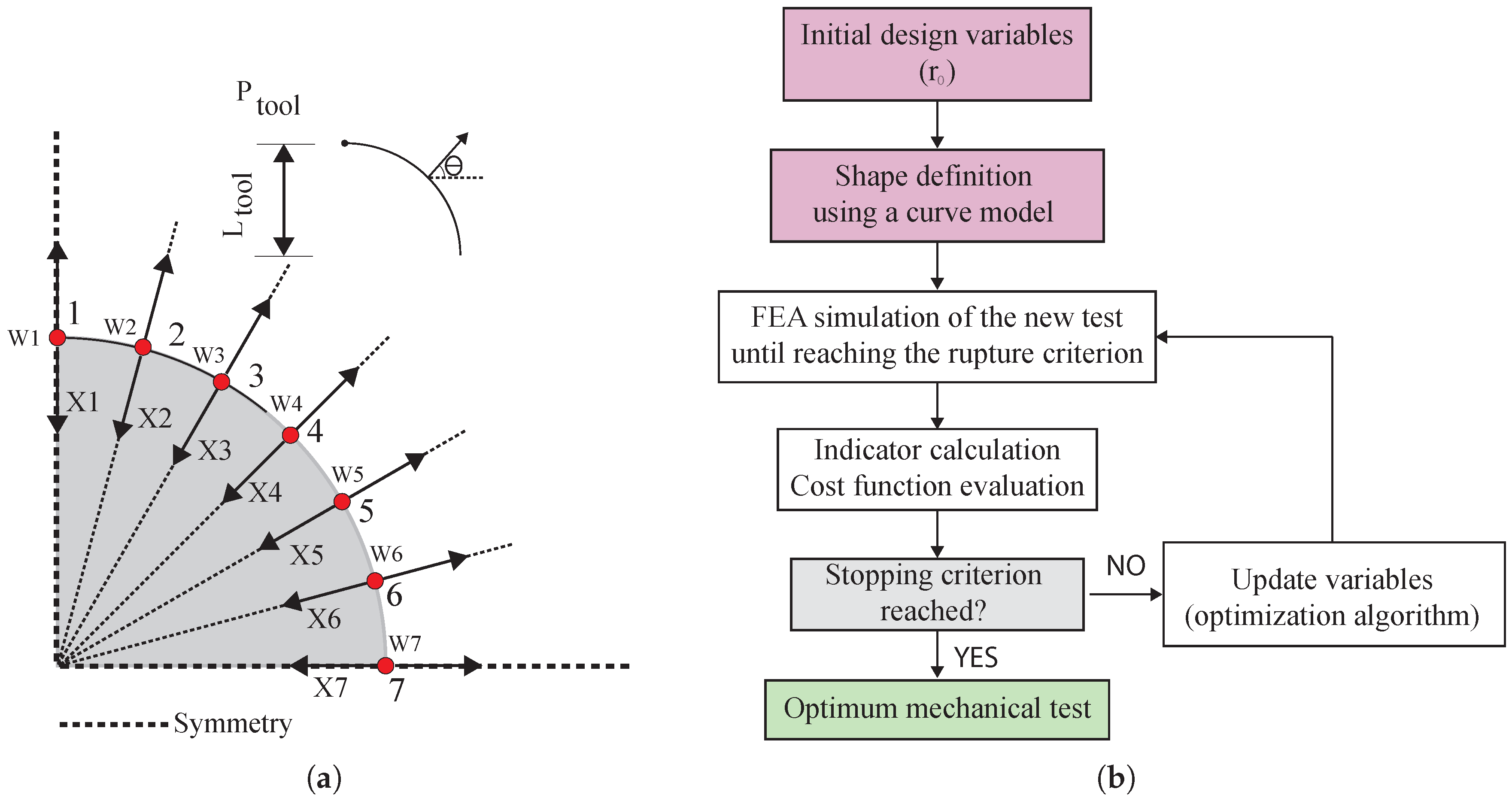
3. Optimization Features and Geometry Definition

3.1. Geometry Definition Using a Curve Model

Different curve models are used to describe, parameterize, and control the specimen geometry during the iterative process:

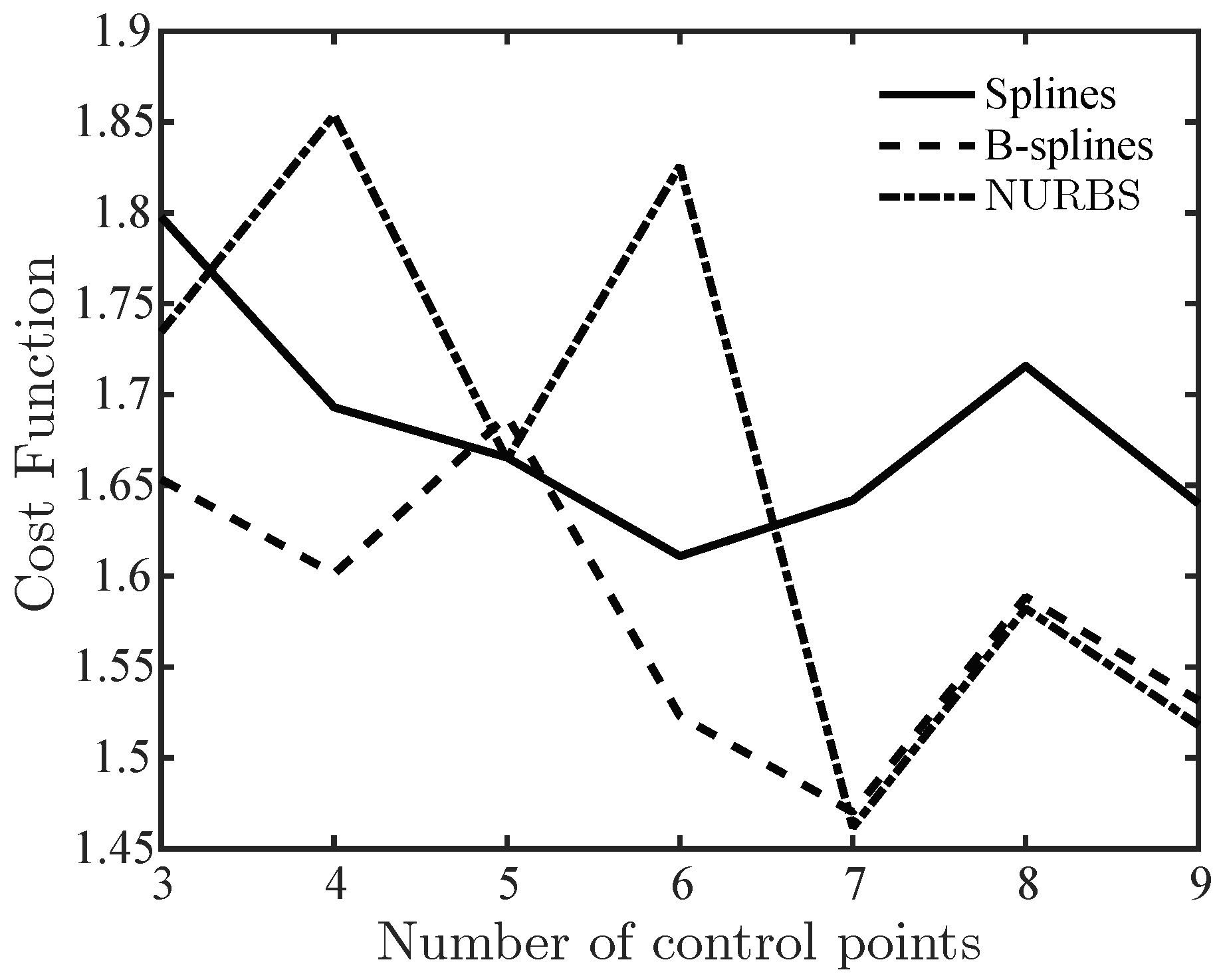
• Cubic splines: Define a curve as a set of connected piecewise simple polynomial functions. The control points are interpolated, and no local control is considered in the geometry, only global. Therefore, abrupt variations can be observed on consecutive control points’ positions during the optimization, leading to unrealistic specimen shapes and to premature strain localization and rupture [4]. In order to avoid this drawback, a penalty function $Res$ to constrain these variations was created. This penalty function is defined by:

  $$Res=\sum _{i=1}^6\alpha ({\left[\max (g_{U,i}\left(r\right),0)\right]}^2+{\left[\max (g_{L,i}\left(r\right),0)\right]}^2),$$

  (2)

  with:

  $$g_{U,i}\left(r\right)=X_{i+1}-(1+a_v)X_i$$

  (3)

  and:

  $$g_{L,i}\left(r\right)=(1-a_v)X_i-X_{i+1},$$

  (4)

  where $\alpha =1/{(U_{\mathrm{bound}}-L_{\mathrm{bound}})}^2$, the parameter $a_v$ defines the admissible variation, and $X_i$ represents the control point.
• B-splines can be set as a single piecewise curve defined as a linear combination of control points $X_i$ and a B-spline basis function $N_{i,k}\left(t\right)$. The B-spline can be described as:

  $$P{\left(t\right)}_{\mathrm{B}-\mathrm{spline}}=\sum _{i=0}^n{X}_i{N}_{i,k}\left(t\right),n\le k-1,t\in [t_{k-1},t_{k+1}].$$

  (5)

  For the $i\mathrm{th}$ normalized B-spline basis function of order k, the basis function $N_{i,k}\left(t\right)$ is defined by:

  $$N_{i,1}\left(t\right)=\left\{\begin{array}{cc}1,\hfill & \mathrm{if}{v}_i\le t\le v_{i+1}\hfill \\ 0,\hfill & \mathrm{otherwise}\hfill \end{array}\right.$$

  (6)

  and:

  $$N_{i,k}\left(t\right)=\frac{(t-v_i)N_{i,k-1}\left(t\right)}{v_{i+k}-v_i}+\frac{(v_{i+k+1}-t)N_{i+1,k-1}\left(t\right)}{v_{i+k+1}-v_{i+1}},$$

  (7)

  where $v_i$ are elements of a knot vector. In this work, B-splines of fourth order are used. Notice that, when using fourth order B-splines, the penalty function (2) is unnecessary because the curve becomes smoother. The knot vector assumes the following form: $V=(0,0,0,0,t_k,\dots ,t_i,1,1,1,1)$, where n + 1 is the number of control points;
• NURBS are functions that have the same properties as B-splines and are capable of representing a wider class of geometries. A NURBS curve is represented as a combination of control points and rotational basis functions $R_{i,k}\left(t\right)$ and can be defined by:

  $$P{\left(t\right)}_{\mathrm{nurbs}}=\sum _{i=1}^n{X}_i{R}_{i,k}\left(t\right)$$

  (8)

  with:

  $$X_i{R}_{i,k}\left(t\right)=\frac{W_i{N}_{i,k}\left(t\right)}{{\sum }_{i=1}^n{W}_i{N}_{i,k}\left(t\right)},$$

  (9)

  where $W_i>0$ is a weighting factor for the control points. If the weights of the control points are equal to one, the resulting curve is a B-spline. For more details concerning curve models, see [19].

3.2. Numerical Method and Test Design

The design of the heterogeneous test resorts to a shape optimization problem. In order to balance the loads in the transversal directions, the design methodology uses a symmetric model (Figure 1a). In this model, the design variables are the n control points’ positions $X_i=[X_1,\dots ,X_n]$ that define the specimen’s initial shape (before deformation) and weights $W_i=[W_1,\dots ,W_n]$ and the rigid tool length $L_{\mathrm{tool}}$. The tool length defines only the size of the tool. The shape of the tool is defined by the boundary of the specimen. As shown in Figure 1a, each control point is spaced radially by ${90}^{°}/(n-1)$. It was defined that the control points only change their radial position. In each design iteration, the specimen geometry and loading path are allowed to change freely, limited uniquely by the design variables’ boundaries. The search universe of the design variables is given by $X_i\in [10,60]\mathrm{mm}$ and $W_i\in [0.5,20]$.

The optimization of the loading path depends on the design of the rigid tool. To avoid symmetry conflicts, the tool needs to be coincident with the specimen shape and the beginning point $P_{\mathrm{tool}}$ to be at ${90}^{°}$, which means that the orientation of the tool displacement $\theta$ will be ${90}^{°}$ due to the symmetry. The loading path is applied up to rupture, established by $W_{\mathrm{CL}}^{\mathrm{f}}$. During the process, the optimization algorithm automatically modifies the specimen shape until reaching a stopping criterion. In each FEA evaluation, the mesh is automatically adapted to the specimen. However, whatever the specimen size, the number of elements remains constant.

This iterative process was launched using a MATLAB-Python-Abaqus environment. In MATLAB, the initial coordinates $R_0=\{X_0,W_0,P_{\mathrm{tool}}\}$ of the design variables, the optimization algorithm, and the curve model definition are specified. A script developed in Python is able to read the defined geometry and to update it. The numerical simulation was carried out up to rupture by Abaqus [20]. The output result was also post-processed using a Python script, enabling calculation of the indicator $I_{\mathrm{T}}$ and cost function. Based on the final result, the process may end if a stopping criterion is reached or continues to update the design variables’ coordinates iteratively. This iterative design optimization problem can be formulated as:

$$\begin{array}{ll}{\displaystyle \underset{R=\{X_i,W_i,P_{\mathrm{tool}}\}}{min}}\hfill & f\left(R\right)=2-I_{\mathrm{T}}+Res\hfill \end{array}$$

(10)

$$\begin{array}{ll}\mathrm{subject}\mathrm{to}:\hfill & 10\le X_i\le 60\mathrm{mm}\hfill \\ & {10}^{°}\le {\mathrm{P}}_{\mathrm{tool}}\le {90}^{°}\hfill \\ & 0.5\le W_i\le 20(\mathrm{for}\mathrm{NURBS})\hfill \\ & W_i=1(\mathrm{for}\mathrm{B}-\mathrm{Splines})\hfill \\ & W_i=\nexists (\mathrm{for}\mathrm{splines}).\hfill \end{array}$$

(11)

Following the established numerical procedure (Figure 1b), the outcome revealed to be dependent on:

• The geometry definition and discretization: This feature is related to the numerical simulation, the number of elements, the number of control points used, the curve model, the parametrization used, etc.
• The optimization method: This defines the robustness of the process and can influence the final result.
• The cost function parameters: A modification of these parameters can lead to different results. A very robust cost function can provide better results. However, this is not the object of study in this work.

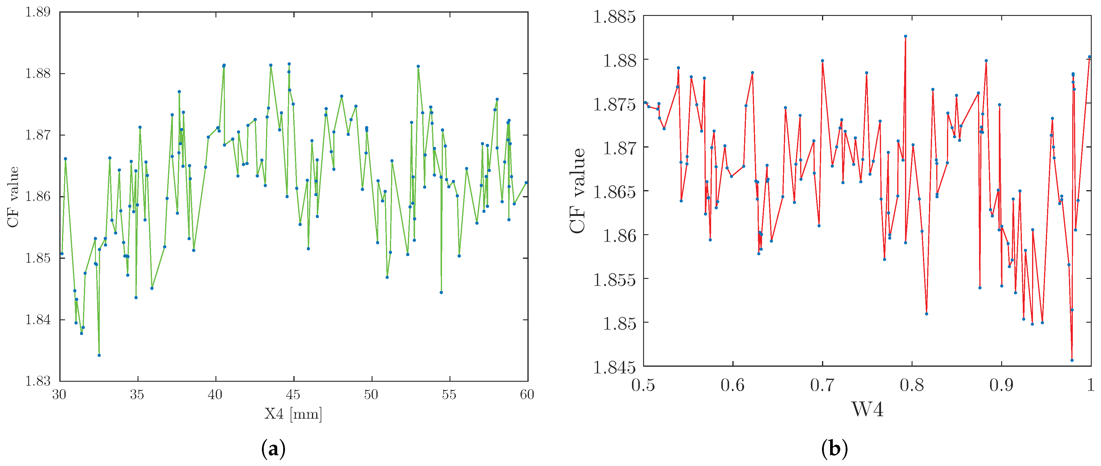
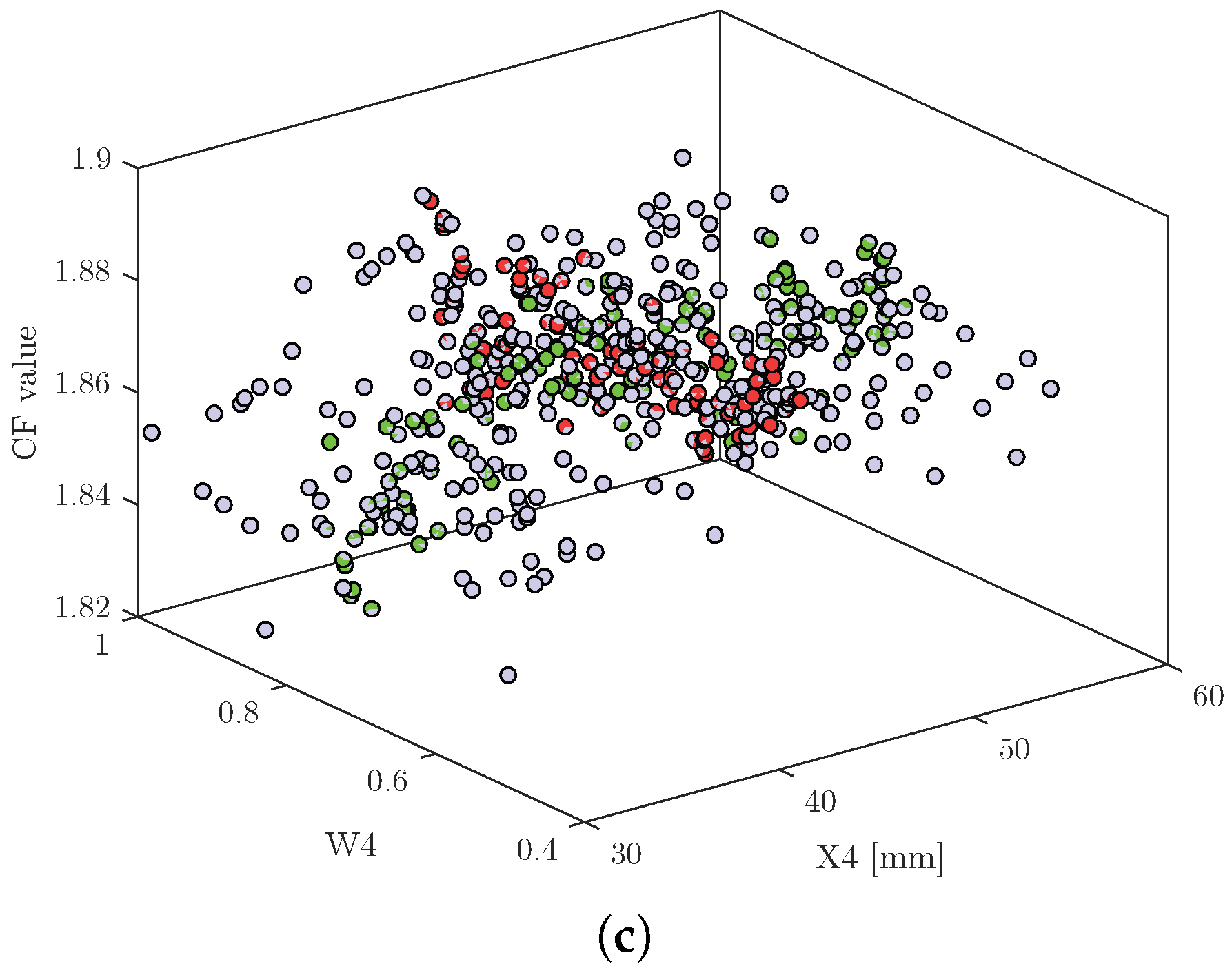
3.3. Number of Control Points and Sensitivity Analysis

The geometry of the specimen is defined by the control points’ positions, which means that the number of control points used has an influence on the design process. To obtain a non-linear design process independent of the number of control points, the optimum control parametrization Ritz method was used [21]. In this method, the number of control points is progressively increased until convergence to an optimum value. In this work, the iterative process was executed for each curve model starting with three control points, using the SDBOX [22] optimization technique.

Due to the black-box nature of this problem, the derivatives are not available. The sensitivity analysis of the cost function allows analyzing the contribution of a variable to the cost function, showing how it behaves when the variables’ values change. The derivative information can be obtained using approximation methods, such as finite differences, when the cost function behaves as a smooth continuous function. This would widen the range of applicable optimization algorithms. However, the output of the objective function value is dependent on a FEA. As the mesh generation is random, even when applying fine meshes, the output result will always have small discrete variations, which can lead to noisy data. In this work, the One-At-a-Time (OAT/OFAT) method was used to perform a sensitivity analysis of the cost function [1,23], where the contributions were determined by varying a parameter, while keeping all the others constant. The initial configuration shown in Figure 1 and Control Point 4 were selected for the sensitivity analysis.

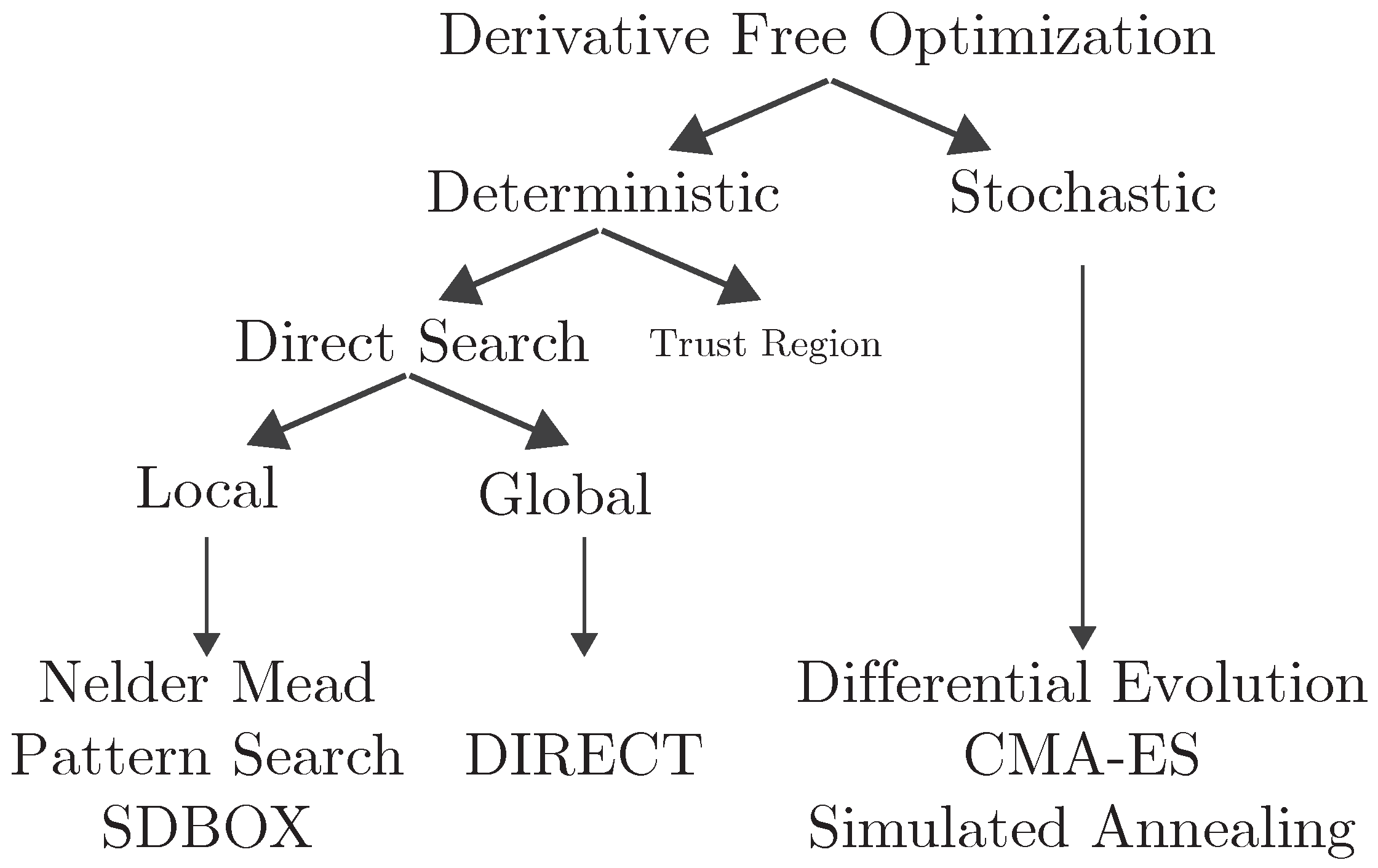
3.4. Optimization Strategy

One of the goals of this work is to find an optimization algorithm capable of robustly minimizing the objective function. The performance of the optimization algorithm is evaluated by the time and the number of function evaluations required to converge. According to the sensitivity analysis results (see Section 4.1), the cost function is non-smooth and (possibly) multi-modal. Therefore, the solution lies in finding suitable Derivative-Free Optimization (DFO) methods to solve the optimization problem [22,24]. The recently-developed DFO methods are either deterministic or stochastic. Figure 2 classifies the optimization methods according to their categories.

Direct search methods are deterministic and can be described as a continuous examination of the outcome results generated by the optimization strategy. The local direct search algorithms are dependent on the initial parameters and conditions and are susceptible to local minima [25]. However, these methods have a fast convergence. Global search optimization methods, such as Lipschitzian-based partitioning methods, provide theoretical guarantees of finding the global minimum of an optimization problem within a certain tolerance. In stochastic optimization, randomness is part of the search procedure for the global optimum. Most of the methods are based on population/swarm intelligence and mimic the behavior of natural systems. Such algorithms are less prone to getting trapped in local minima. However, the convergence is commonly much slower [26,27]. In this work, seven optimization strategies were used; however, only four were able to converge to a solution: the Nelder–Mead, pattern search, SDBOX, and CMA-ES.

3.4.1. CMA-ES

The Covariance Matrix Adaptation Evolutionary Strategy (CMA-ES) is an evolutionary algorithm proposed by Nikolaus Hansen and Andreas Ostermeier [28]. CMA-ES is a second order approach and creates a Gaussian probabilistic model of possible solutions. The new candidate solutions are sampled according to a multivariate normal distribution, and the mutation acts as a perturbation with zero mean. In this particular algorithm, pairwise dependencies between the variables in the distribution are represented by a covariance matrix that is updated progressively. This process will then influence the next generation [24,28].

3.4.2. SDBOX

To guarantee both global convergence and robustness, this optimization strategy has roots in gradient-based methods. This algorithm is able to detect the coordinate direction that minimizes the cost function by investigating the local behavior. To create a new point, the algorithm performs a line-search along the found coordinate direction. The iterations’ information can be used to build an approximation of the cost function [22].

3.4.3. Nelder–Mead

Nelder–Mead is a direct search algorithm based on a spacial approximation. It consists of the definition of a non-degenerate simplex [24]. For an objective function containing r variables, this algorithm retrieves the convex hull of $r+1$ vertices. In each iteration, it removes the vertex with the worst objective function value. Then, it updates it to a better value by reflecting, expanding, or contracting the simplex along the joint line with the centroids of the remaining vertices. This algorithm usually requires a low number of function evaluations before finding the minimum. However, if the function is multi-modal, it becomes dependent on the initial shape of the specimen, as it gets trapped in the local minima.

3.4.4. Pattern Search

Pattern search is a direct search method proposed by Hooke and Jeeves. It involves two types of moves: (i) exploratory search, which is a local search step that looks for an improving direction, and (ii) pattern move, where, after a chosen direction, it tries larger moves in the improving direction. The implemented pattern search uses Mesh Adaptive Direct Search (MADS), which removes the restrictions of general pattern search to finitely-selected directions, allowing local analysis in a dense set of directions in the space of design variables [29].

4. Results and Discussion

4.1. Ritz Method and Sensitivity Analysis

Figure 3 shows the outcomes of the Ritz method. Unlike what was expected, a full convergence with the increase of control points was not observed. The use of a higher number of control points allows the representation of a wider class of geometries. However, the number of local minima of the cost function can also increase and, consequently prevent the full convergence of the optimization method. Furthermore, the number of design variables was higher, which may have led to unrealistic geometries, resulting in simulations that did not converge to a solution. Even without full convergence, Figure 3 shows the number of control points that should be used for each curve model definition: seven control points for B-splines and NURBS and six for splines.

Figure 4 shows the behavior of the cost function in response to small perturbations of the position and weight values. The function exhibits a non-smooth and non-continuous behavior, demonstrating that gradient-based methods cannot be used.

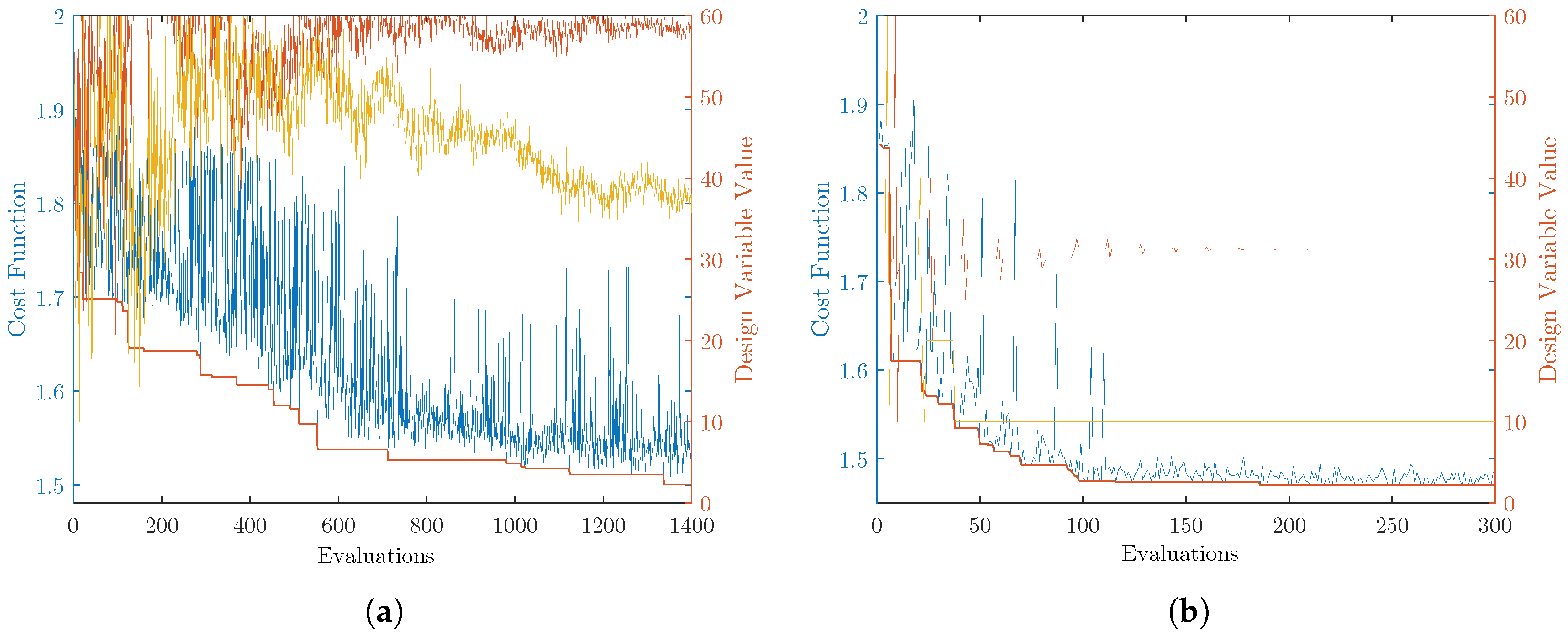
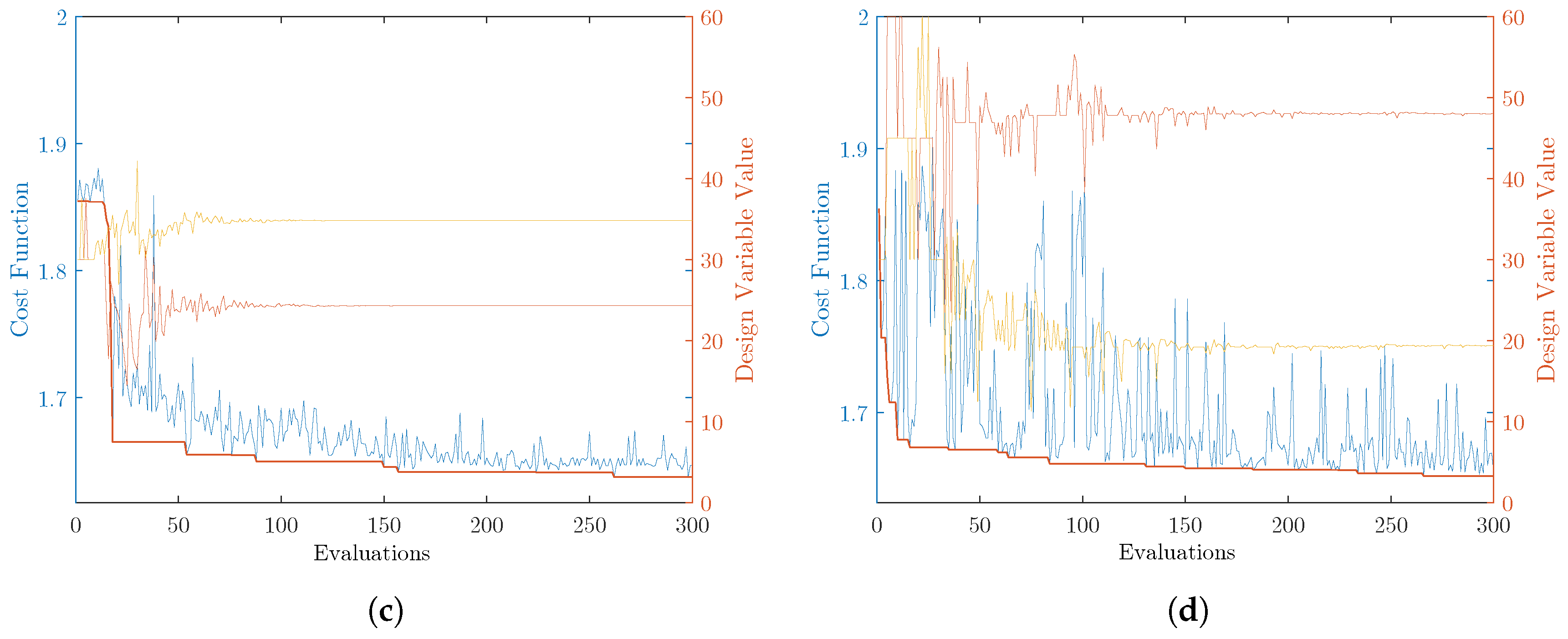
4.2. Optimization Algorithms Performance Evaluation

The results were obtained by combining the optimization algorithms with the curve models. The aim was to find a combination capable of robustly minimizing the cost function and, consequently, provide a specimen design. The optimization algorithms’ performance was based on two criteria: the best CF value and the convergence rate. Figure 5 shows the convergence rate of the cost function and the evolution of two design variables, allowing us to observe the differences between their behaviors. The direct search algorithms were faster to converge to a solution. The Nelder–Mead had a smoother convergence curve because it promotes small modifications in the design variables between iterations. Pattern search performed more abrupt modifications, which led to an irregular cost function minimization. SDBOX revealed a good compromise between efficiency and convergence properties. As expected for stochastic algorithms, CMA-ES presented large oscillations; however, it reached the lowest cost function value.

Concerning the design variables, in the first evaluations, large oscillations were observed. The design variables reached the search universe boundaries, and with the reduction and convergence of the cost function, their convergence was attained, even if it converged to a local minimum.

CMA-ES was, along with SDBOX, the algorithm that reached the best results; however, a much higher number of iterations was required. Notice that after 1000 function evaluations, the design variables were still converging.

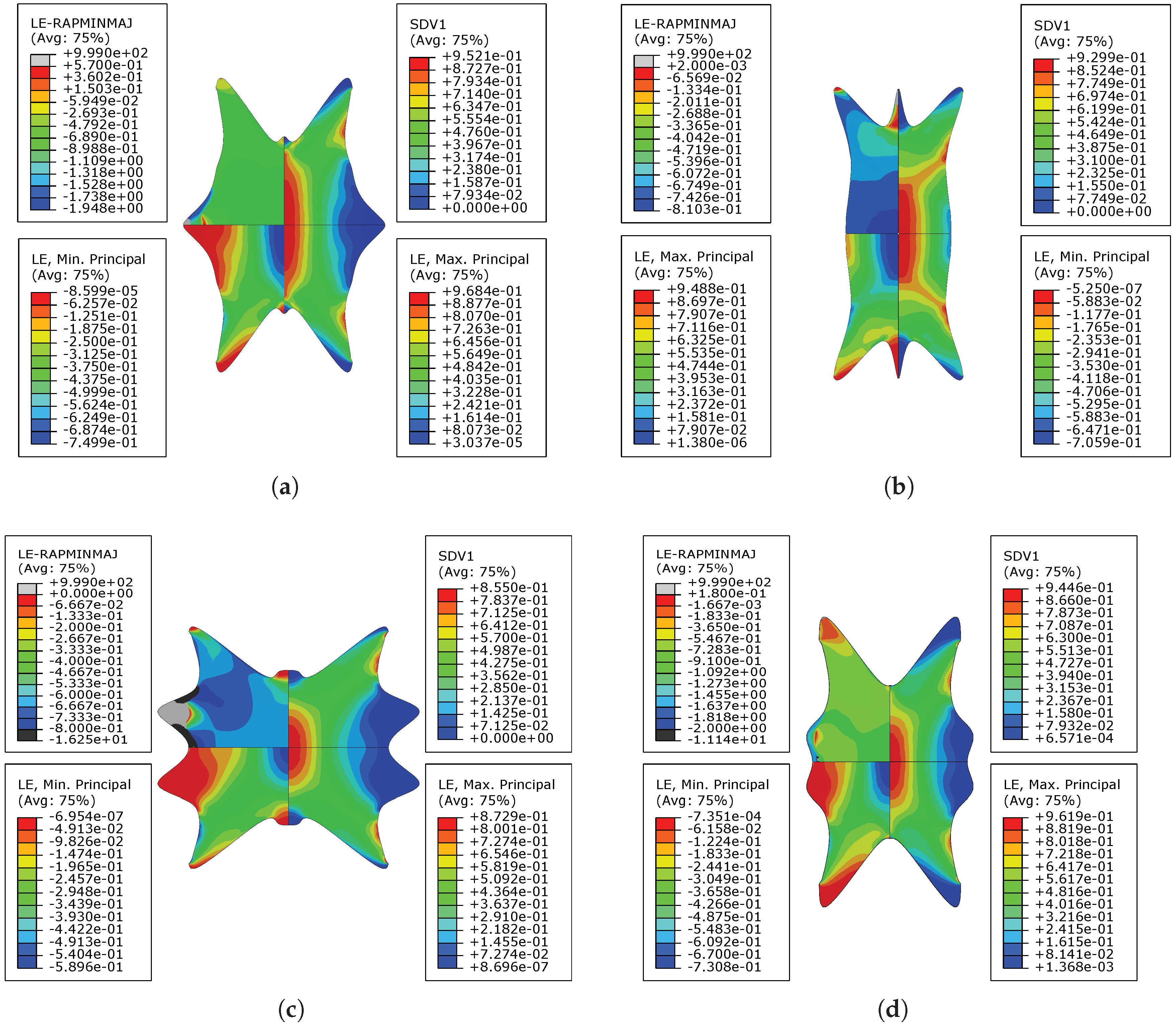
4.3. Test Design: Optimization Results

Table 6. Results for the mechanical test design using different optimization strategies and boundary curve models.

B-Splines	CMA-ES	Nelder	Pattern	SDBOX
		Mead	Search
$W_{\mathrm{r}1}{\displaystyle \frac{\mathrm{Mean}\left[\mathrm{Std}({\epsilon }_2/{\epsilon }_1)\right]}{W_{\mathrm{a}1}}}$	0.0273	0.0438	0.0249	0.0327
$W_{\mathrm{r}2}{\displaystyle \frac{{({\epsilon }_2/{\epsilon }_1)}_r}{W_{\mathrm{a}2}}}$	0.0100	0.0115	0.0092	0.0109
$W_{\mathrm{r}3}{\displaystyle \frac{\mathrm{Mean}\left[\mathrm{Std}\left({\overline{\epsilon }}^{\mathrm{P}}\right)\right]}{W_{\mathrm{a}3}}}$	0.1277	0.0908	0.0747	0.1345
$W_{\mathrm{r}4}{\displaystyle \frac{{\overline{\epsilon }}_{\mathrm{Max}}^{\mathrm{P}}}{W_{\mathrm{a}4}}}$	0.1070	0.0897	0.0864	0.1021
$W_{\mathrm{r}5}{\displaystyle \frac{A{v}_{{\overline{\epsilon }}^{\mathrm{P}}}}{W_{\mathrm{a}5}}}$	0.2273	0.1178	0.1455	0.2352
CF Minimum	1.5007	1.6464	1.6592	1.4846
${\overline{\epsilon }}_{\mathrm{tensile}}^{\mathrm{P}}$	0.5346	0.3231	0.3674	0.4108
${\overline{\epsilon }}_{\mathrm{biaxial}}^{\mathrm{P}}$	0	0	0	0
${\overline{\epsilon }}_{\mathrm{shear}}^{\mathrm{P}}$	0.0102	0.0038	0.0012	0.0145
${\overline{\epsilon }}_{\mathrm{plane}}^{\mathrm{P}}$	0.0012	0.0149	0.0302	0.0042
${\overline{\epsilon }}_{\mathrm{comp}}^{\mathrm{P}}$	0.0154	0.0141	0.0094	0.0274
${\overline{\epsilon }}_{\mathrm{test}}^{\mathrm{P}}$	0.9058	0.8741	0.7761	0.9439
NURBS	CMA-ES	Nelder	Pattern	SDBOX
		Mead	Search
$W_{\mathrm{r}1}{\displaystyle \frac{\mathrm{Mean}\left[\mathrm{Std}({\epsilon }_2/{\epsilon }_1)\right]}{W_{\mathrm{a}1}}}$	0.0313	0.0448	0.0357	0.0163
$W_{\mathrm{r}2}{\displaystyle \frac{{({\epsilon }_2/{\epsilon }_1)}_r}{W_{\mathrm{a}2}}}$	0.0138	0.0098	0.0082	0.0041
$W_{\mathrm{r}3}{\displaystyle \frac{\mathrm{Mean}\left[\mathrm{Std}\left({\overline{\epsilon }}^{\mathrm{P}}\right)\right]}{W_{\mathrm{a}3}}}$	0.1465	0.0699	0.0970	0.1098
$W_{\mathrm{r}4}{\displaystyle \frac{{\overline{\epsilon }}_{\mathrm{Max}}^{\mathrm{P}}}{W_{\mathrm{a}4}}}$	0.1069	0.0807	0.0972	0.1047
$W_{\mathrm{r}5}{\displaystyle \frac{A{v}_{{\overline{\epsilon }}^{\mathrm{P}}}}{W_{\mathrm{a}5}}}$	0.2634	0.0991	0.1391	0.3050
CF Minimum	1.4380	1.6956	1.6228	1.4601
${\overline{\epsilon }}_{\mathrm{tensile}}^{\mathrm{P}}$	0.4517	0.2323	0.4469	0.4628
${\overline{\epsilon }}_{\mathrm{biaxial}}^{\mathrm{P}}$	0	0	0	0
${\overline{\epsilon }}_{\mathrm{shear}}^{\mathrm{P}}$	0.0112	0.0055	0.0024	0
${\overline{\epsilon }}_{\mathrm{plane}}^{\mathrm{P}}$	0.0282	0.0359	0.0184	0.0501
${\overline{\epsilon }}_{\mathrm{comp}}^{\mathrm{P}}$	0.0244	0.0055	0.0208	0
${\overline{\epsilon }}_{\mathrm{test}}^{\mathrm{P}}$	0.9502	0.8281	0.8446	0.9226
Splines	CMA-ES	Nelder	Pattern	SDBOX
		Mead	Search
$W_{\mathrm{r}1}{\displaystyle \frac{\mathrm{Mean}\left[\mathrm{Std}({\epsilon }_2/{\epsilon }_1)\right]}{W_{\mathrm{a}1}}}$	0.0293	0.0347	0.0364	0.0319
$W_{\mathrm{r}2}{\displaystyle \frac{{({\epsilon }_2/{\epsilon }_1)}_r}{W_{\mathrm{a}2}}}$	0.0120	0.0094	0.0082	0.0105
$W_{\mathrm{r}3}{\displaystyle \frac{\mathrm{Mean}\left[\mathrm{Std}\left({\overline{\epsilon }}^{\mathrm{P}}\right)\right]}{W_{\mathrm{a}3}}}$	0.0970	0.0853	0.0884	0.0889
$W_{\mathrm{r}4}{\displaystyle \frac{{\overline{\epsilon }}_{\mathrm{Max}}^{\mathrm{P}}}{W_{\mathrm{a}4}}}$	0.0931	0.0865	0.0849	0.0927
$W_{\mathrm{r}5}{\displaystyle \frac{A{v}_{{\overline{\epsilon }}^{\mathrm{P}}}}{W_{\mathrm{a}5}}}$	0.1943	0.1546	0.1349	0.1649
CF Minimum	1.5741	1.6294	1.6472	1.6110
${\overline{\epsilon }}_{\mathrm{tensile}}^{\mathrm{P}}$	0.3543	0.3460	0.2944	0.3421
${\overline{\epsilon }}_{\mathrm{biaxial}}^{\mathrm{P}}$	0	0	0	0
${\overline{\epsilon }}_{\mathrm{shear}}^{\mathrm{P}}$	0.0047	0.00134	0.0080	0.0073
${\overline{\epsilon }}_{\mathrm{plane}}^{\mathrm{P}}$	0.0271	0.0812	0.0055	0.0573
${\overline{\epsilon }}_{\mathrm{comp}}^{\mathrm{P}}$	0.0204	0.00851	0.0191	0.0147
${\overline{\epsilon }}_{\mathrm{test}}^{\mathrm{P}}$	0.8500	0.83976	0.8370	0.8501

shows the results for the sets curve-models/optimization-algorithms. The direct search local algorithms presented similar values for the different models, showing a fast convergence to a local minimum. Regarding the global optimization algorithms, a good ability to decrease the cost function value was observed, and the solutions revealed to be inferior (better) to the ones obtained by local search. However, this was not observed with the use of splines. For this curve model, the values of the cost function were very similar for all optimization algorithms, evidencing proximity between the global and the local minima of the function. Both NURBS and B-splines presented clear differences when using global or local optimization algorithms. It is also important to highlight that more than one global minimum can exist. The final values of each term of the cost function obtained using the evolutionary algorithm CMA-ES and the direct search algorithm SDBOX were different, yet the cost function values were very close.

When analyzing the results, particularly the final cost functions for each test, four candidate solutions were identified: (a) CMA-ES with B-splines, (b) SDBOX and B-splines, (c) CMA-ES with NURBS, and (d) SDBOX with NURBS. Figure 6 shows the deformed state and the strain distributions over the deformed specimen. Regarding the strain state range, the solution provided by SDBOX with NURBS revealed to be limited due to the inability to reach some of the relevant strain states. However, it presented the best value concerning the overall plastic deformation, represented by $A{v}_{{\overline{\epsilon }}^{\mathrm{P}}}$. The mean deformation heterogeneity $Mean\left[std({\epsilon }_2/{\epsilon }_1)\right]$ and the maximum strain achieved ${\overline{\epsilon }}_{\mathrm{Max}}^{\mathrm{P}}$ in these tests were identical. Nonetheless, none of the tests were capable of producing the biaxial strain state.

Considering that the solutions identified by global optimization algorithms can be exploratory values and not minima, a local search algorithm was used in each candidate solution. However, no improvements were noticed, demonstrating that the results attained by the global optimization algorithm were minima.

Figure 7 presents the strain state range offered by each solution represented in Figure 6. Although all solutions widened the strain states provided by classical homogeneous tests, most strain states fit in the neighborhood of uniaxial tension. This was expected due to the tensile load conditions of the tests and constitutes a limitation of the presented methodology. Other load conditions would present different strain states, but could also require a more complex apparatus than a standard uniaxial load test machine. The solutions (b) and (c) presented shear and uniaxial compression states, but only for small values of strains. Taking into account these analyzes and the CF value, the solution provided in (c) CMA-ES with NURBS revealed to be the most promising.

5. Conclusions

In this work, a shape optimization process was applied to design a heterogeneous test for the mechanical characterization of sheet metals under multiple strain paths and strain amplitudes. To describe the shape of the specimen, the test was subjected to optimization using both splines, B-splines, and NURBS. With the purpose of improving the efficiency of the design process, a Ritz-type method was applied to optimize the number of control points used in each curve model. The specimen capable of providing more mechanical information was reached by using NURBS with CMA-ES. Quantitatively, this kind of curve model appeared to be the most effective one in finding a heterogeneous test that promotes a better mechanical characterization of sheet metals. However, the CMA-ES optimization model can be considered as good as the SDBOX, as the results obtained with the latter were similar and presented a 10-times faster convergence.

All the specimen shapes obtained by the design optimization process were quite similar, presenting variations in both the length and width of the specimen, which promote the heterogeneities of the strain field. Such specimens revealed profiles similar to butterflies. Although butterfly-type specimens have been used in the past for a range of stress states from simple shear to plane-strain tension [30,31] using multiple tests, the specimens presented here displayed a wider range of stress states for a single test.

The design methodology presented in this paper achieved novel geometries that offer wider ranges of stress/strain states than the classical or the actual heterogeneous tests. Therefore, it constitutes a state-of-the-art improvement. However, it has not reached yet a unique test presenting both the overall range of stress/strain states and large levels of plastic strains. This fact can be due to the limitation in the loading conditions and in the shape definition, opening challenges for future works.

References

1. Ablat, M.A.; Qattawi, A. Numerical simulation of sheet metal forming: A review. Int. J. Adv. Manuf. Technol. 2016, 1235–1250. [Google Scholar] [CrossRef]
2. Teaca, M.; Charpentier, I.; Martiny, M.; Ferron, G. Identification of sheet metal plastic anisotropy using heterogeneous biaxial tensile tests. Int. J. Mech. Sci. 2010, 52, 572–580. [Google Scholar] [CrossRef]
3. Zhang, S.; Leotoing, L.; Guines, D.; Thuillier, S. Potential of the Cross Biaxial Test for Anisotropy Characterization Based on Heterogeneous Strain Field. Exp. Mech. 2015, 55, 817–835. [Google Scholar] [CrossRef] [Green Version]
4. Souto, N. Computational Design of a Mechanical Test for Material Characterization by Inverse Analysis. Ph.D. Thesis, University of Aveiro, Aveiro, Portugal, 2015. [Google Scholar]
5. Avril, S.; Bonnet, M.; Bretelle, A.S.; Grédiac, M.; Hild, F.; Ienny, P.; Latourte, F.; Lemosse, D.; Pagano, S.; Pagnacco, E.; et al. Overview of identification methods of mechanical parameters based on full-field measurements. Exp. Mech. 2008, 48, 381–402. [Google Scholar] [CrossRef]
6. Syed-Muhammad, K.; Toussaint, E.; Grédiac, M. Optimization of a mechanical test on composite plates with the virtual fields method. Struct. Multidiscip. Optim. 2009, 38, 71–82. [Google Scholar] [CrossRef]
7. Souto, N.; Andrade-Campos, A.; Thuillier, S. Mechanical design of a heterogeneous test for material parameters identification. Int. J. Mater. Form. 2017, 10, 353–367. [Google Scholar] [CrossRef]
8. Helfrick, M.N.; Niezrecki, C.; Avitabile, P.; Schmidt, T. 3D digital image correlation methods for full-field vibration measurement. Mech. Syst. Signal Process. 2011, 25, 917–927. [Google Scholar] [CrossRef]
9. Meuwissen, M.; Oomens, C.; Baaijens, F.; Petterson, R.; Janssen, J. Determination of the elasto-plastic properties of aluminium using a mixed numerical–experimental method. J. Mater. Process. Technol. 1998, 75, 204–211. [Google Scholar] [CrossRef]
10. Banabic, D.; Barlat, F.; Cazacu, O.; Kuwabara, T. Advances in anisotropy and formability. Int. J. Mater. Form. 2010, 3, 165–189. [Google Scholar] [CrossRef]
11. Pottier, T.; Vacher, P.; Toussaint, F.; Louche, H.; Coudert, T. Out-of-plane Testing Procedure for Inverse Identification Purpose: Application in Sheet Metal Plasticity. Exp. Mech. 2012, 52, 951–963. [Google Scholar] [CrossRef]
12. Souto, N.; Thuillier, S.; Andrade-Campos, A. Design of an indicator to characterize and classify mechanical tests for sheet metals. Int. J. Mech. Sci. 2015, 101–102, 252–271. [Google Scholar] [CrossRef]
13. Prates, P.A.; Pereira, A.F.G.; Sakharova, N.A.; Oliveira, M.C.; Fernandes, J.V. Inverse Strategies for Identifying the Parameters of Constitutive Laws of Metal Sheets. Adv. Mater. Sci. Eng. 2016, 2016, 4152963. [Google Scholar] [CrossRef]
14. Aquino, J.; Andrade Campos, A.; Souto, N.; Thuillier, S. Experimental validation of a new heterogeneous mechanical test design. AIP Conf. Proc. 2018, 1960, 090002. [Google Scholar] [Green Version]
15. Souto, N.; Thuillier, S.; Andrade-Campos, A. Design of a mechanical test to characterize sheet metals—Optimization using B-splines or cubic splines. AIP Conf. Proc. 2016, 1769. [Google Scholar] [CrossRef]
16. Aquino, J.; Andrade Campos, A.; Souto, N.; Thuillier, S. On the design of innovative heterogeneous tests using a shape optimization approach. AIP Conf. Proc. 2018, 1960, 110001. [Google Scholar]
17. Souto, N.; Andrade-Campos, A.; Thuillier, S. Material parameter identification within an integrated methodology considering anisotropy, hardening and rupture. J. Mater. Process. Technol. 2015, 220, 157–172. [Google Scholar] [CrossRef]
18. Abedini, A.; Butcher, C.; Rahmaan, T.; Worswick, M. Evaluation and calibration of anisotropic yield criteria in shear Loading: Constraints to eliminate numerical artefacts. Int. J. Solids Struct. 2018, 151, 118–134. [Google Scholar] [CrossRef]
19. Piegl, L.; Tiller, W. The NURBS Book; Springer: Berlin/Heidelberg, Germany, 1997. [Google Scholar]
20. Smith, M. ABAQUS/Standard User’s Manual, Version 6.9; Simulia: Providence, RI, USA, 2009. [Google Scholar]
21. Sirisena, H.; Chou, F. Convergence of the Control Parameterization Ritz Method for Nonlinear Optimal Control Problems. J. Optim. Theory Appl. 1979, 29, 369–382. [Google Scholar] [CrossRef]
22. Lucidi, S.; Sciandrone, M. On the Global Convergence of Derivative-Free Methods for Unconstrained Optimization. SIAM J. Optim. 2002, 13, 97–116. [Google Scholar] [CrossRef] [Green Version]
23. Hamby, D.M. A review of techniques for parameter sensitivity analysis of environmental models. Environ. Monit. Assess. 1994, 32, 135–154. [Google Scholar] [CrossRef] [Green Version]
24. Rios, L.M.; Sahinidis, N.V. Derivative-free optimization: A review of algorithms and comparison of software implementations. J. Glob. Optim. 2013, 56, 1247–1293. [Google Scholar] [CrossRef]
25. Hooke, R.; Jeeves, T.A. “Direct Search” Solution of Numerical and Statistical Problems. J. ACM 1961, 8, 212–229. [Google Scholar] [CrossRef]
26. Liberti, L.; Sergei, K. Comparison of deterministic and stochastic approaches to global optimization. Int. Trans. Oper. Res. 2005, 12, 263–285. [Google Scholar] [CrossRef] [Green Version]
27. Cavazzuti, M. Optimization Methods: From Theory to Design: Scientific and Technological Aspects in Mechanics; Springer: Berlin/Heidelberg, Germany, 2013. [Google Scholar]
28. Hansen, N.; Ostermeier, A. Completely Derandomized Self-Adaptation in Evolution Strategies. Evol. Comput. 2001, 9, 159–195. [Google Scholar] [CrossRef] [Green Version]
29. Audet, C.; Custódio, A.L.; Dennis, J.E. Erratum: Mesh Adaptive Direct Search Algorithms for Constrained Optimization. SIAM J. Optim. 2008, 18, 1501–1503. [Google Scholar] [CrossRef] [Green Version]
30. Mohr, D.; Henn, S. Calibration of Stress-triaxiality Dependent Crack Formation Criteria: A New Hybrid Experimental–Numerical Method. Exp. Mech. 2007, 47, 805–820. [Google Scholar] [CrossRef]
31. Abedini, A.; Butcher, C.; Worswick, M.J. Fracture Characterization of Rolled Sheet Alloys in Shear Loading: Studies of Specimen Geometry, Anisotropy, and Rate Sensitivity. Exp. Mech. 2017, 57, 75–88. [Google Scholar] [CrossRef]
Figure 1. (a) Definition of the design variables (here, for n = 7 and θ = 90 ° , data from [4]) and (b) the general optimization procedure.
Metals 09 00371 g001
Figure 2. Categories of the optimization algorithms.
Metals 09 00371 g002
Figure 3. The final value of cost function using different numbers of control points.
Metals 09 00371 g003
Figure 4. Sensitivity analysis of the Cost Function (CF) value to: (a) the position of the control point X4; (b) the weight of the control point W4; and (c) both sensitivities. Sensitivity analysis using a B-spline model with seven control points.
Metals 09 00371 g004aMetals 09 00371 g004b
Figure 5. Evolution of the cost function and two design parameters during the design optimization process using (a) CMA-ES, (b) SDBOX, (c) Nelder–Mead, and (d) pattern search algorithms and a spline curve model.
Metals 09 00371 g005aMetals 09 00371 g005b
Figure 6. Distribution of ε p , ε 2 / ε 1 (corresponding to SDV1 and LE-RAPMINMAJ, respectively), and the major ε 1 and minor strains ε 2 over the specimens surfaces. (a) CMA-ES and (b) SDBOX with B-splines; (c) CMA-ES and (d) SDBOX with NURBS.
Metals 09 00371 g006
Figure 7. Range of ε 2 / ε 1 values on the specimen surface corresponding to the last stage of the test. (a) CMA-ES and (b) SDBOX with B-splines; (c) CMA-ES and (d) SDBOX with NURBS.
Metals 09 00371 g007