Physical Modelling of Aluminum Refining Process Conducted in Batch Reactor with Rotary Impeller


Abstract
:
1. Introduction
2. Materials and Methods
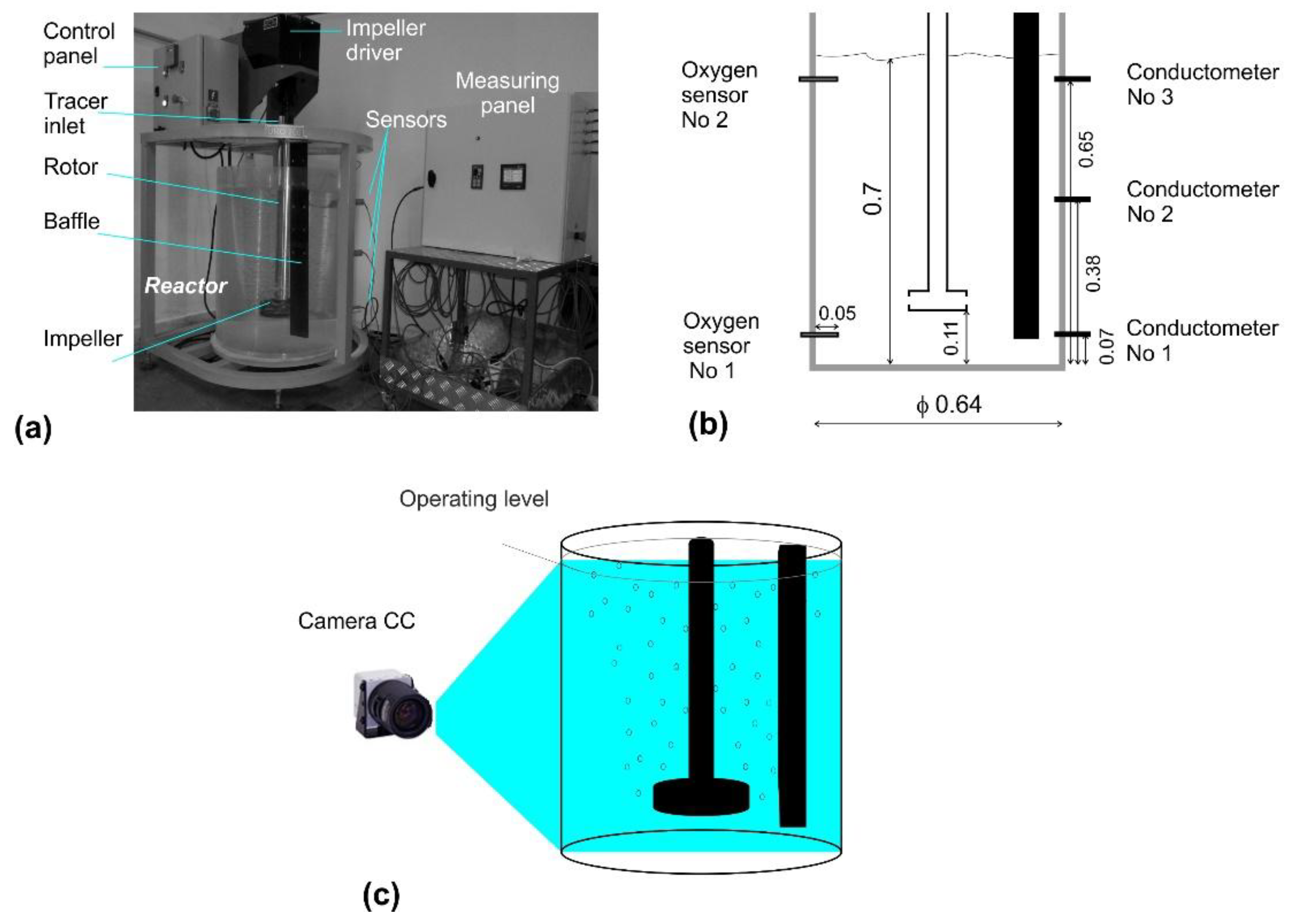
- The model tank was filled with water up to 0.7 m, and the processing parameters were changed according to Table 2.
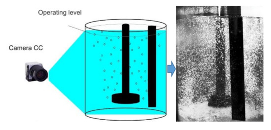
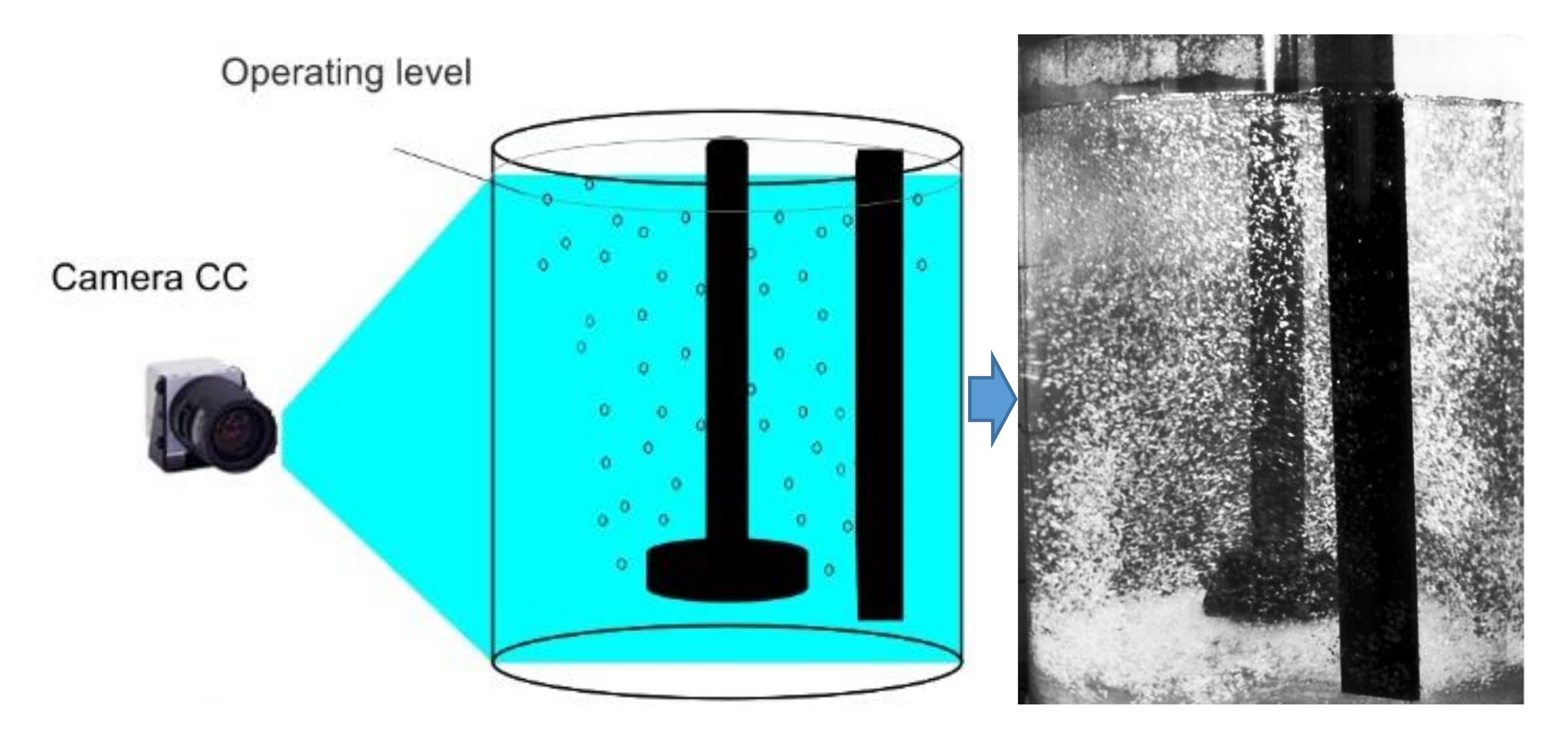
- Visualization research was carried out by digital camera, recording the dispersion level for all rotary impellers, whilst changing the processing parameters.
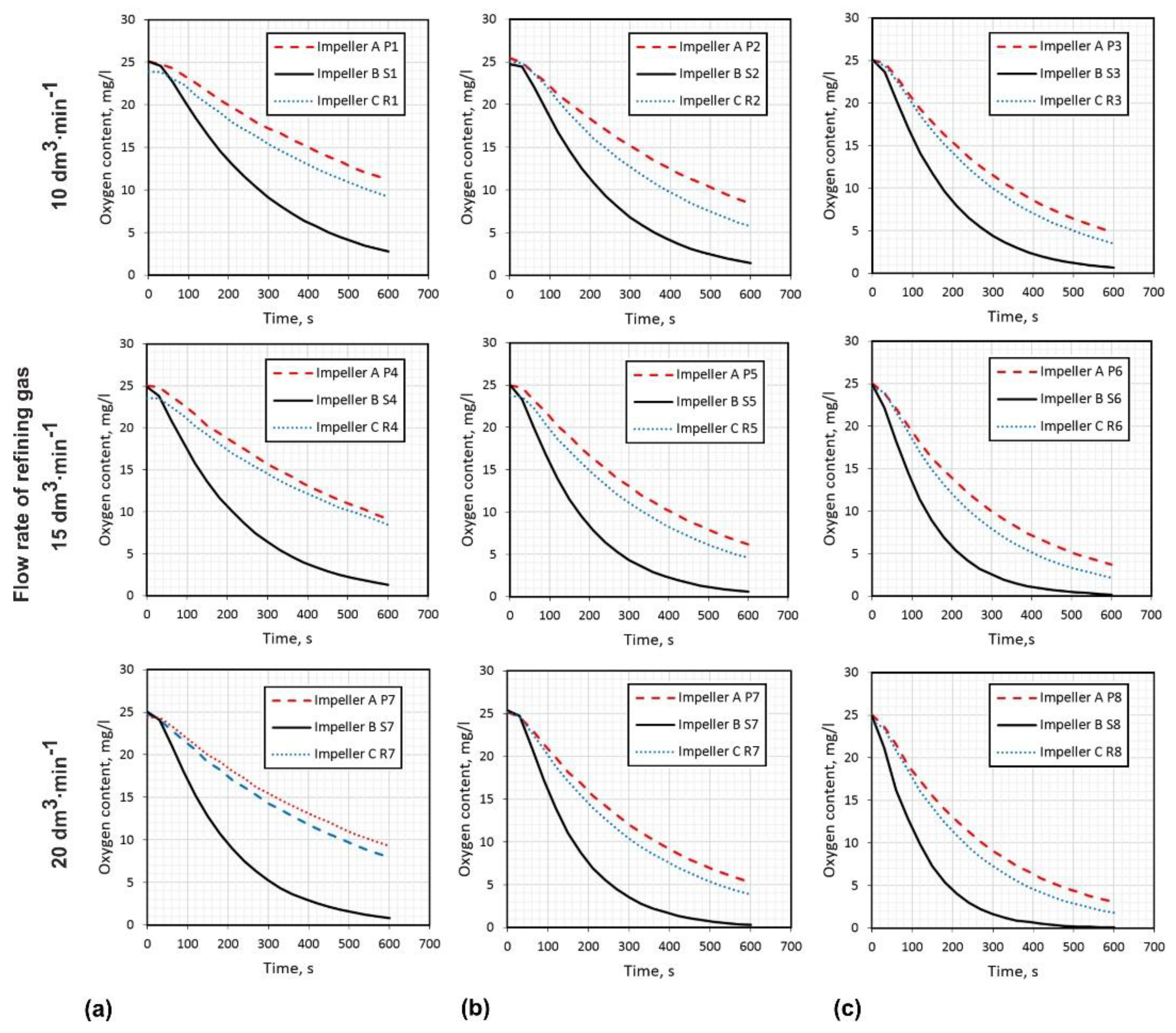
- Next, the tank was saturated with oxygen. The saturation level was measured by two oxygen meters CO-401, Elmetron, Zabrze, Poland (location of oxygen meters is shown in Figure 1b). After reaching the saturation level, argon was introduced into the model by rotary impeller, and processing parameters were according to the variants in Table 2. Removal of oxygen from water, as an analog of hydrogen removal from aluminum [1,22,27], was measured every 0.5 min. The process of aluminum refining in the batch reactor typically lasted 10 min, therefore the process of oxygen removal was carried out for every variant for 10 min.
- Finally, for the selected variants, based on visualization results (dispersion level), RTD curves were measured, the NaCl tracer was poured from the top of the tank with water, the measuring device was switched on, and the three conductometers measured the change in conductivity at three different locations of the reactor model. The obtained results were automatically registered by the computer system.
3. Results and Discussions
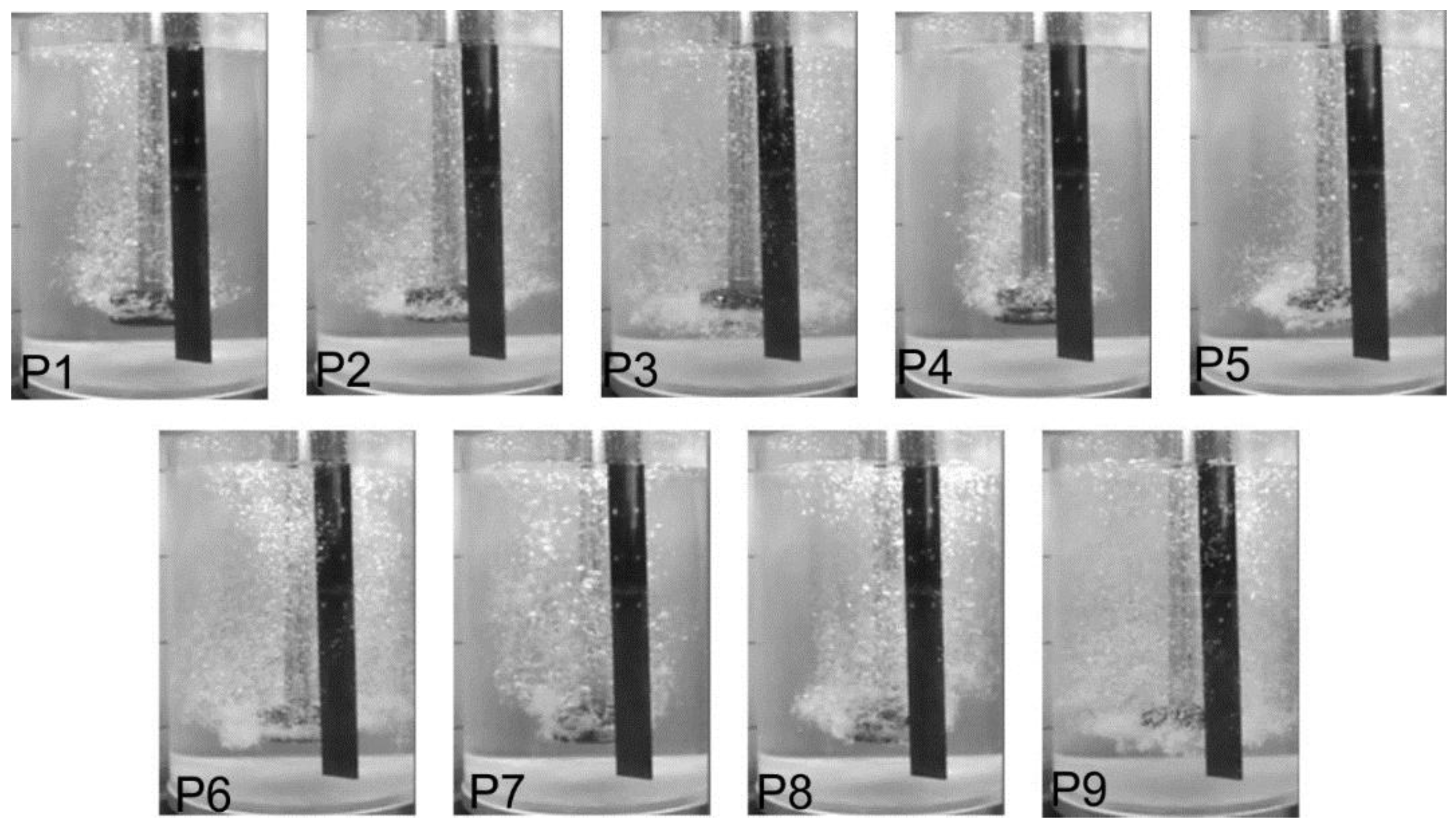
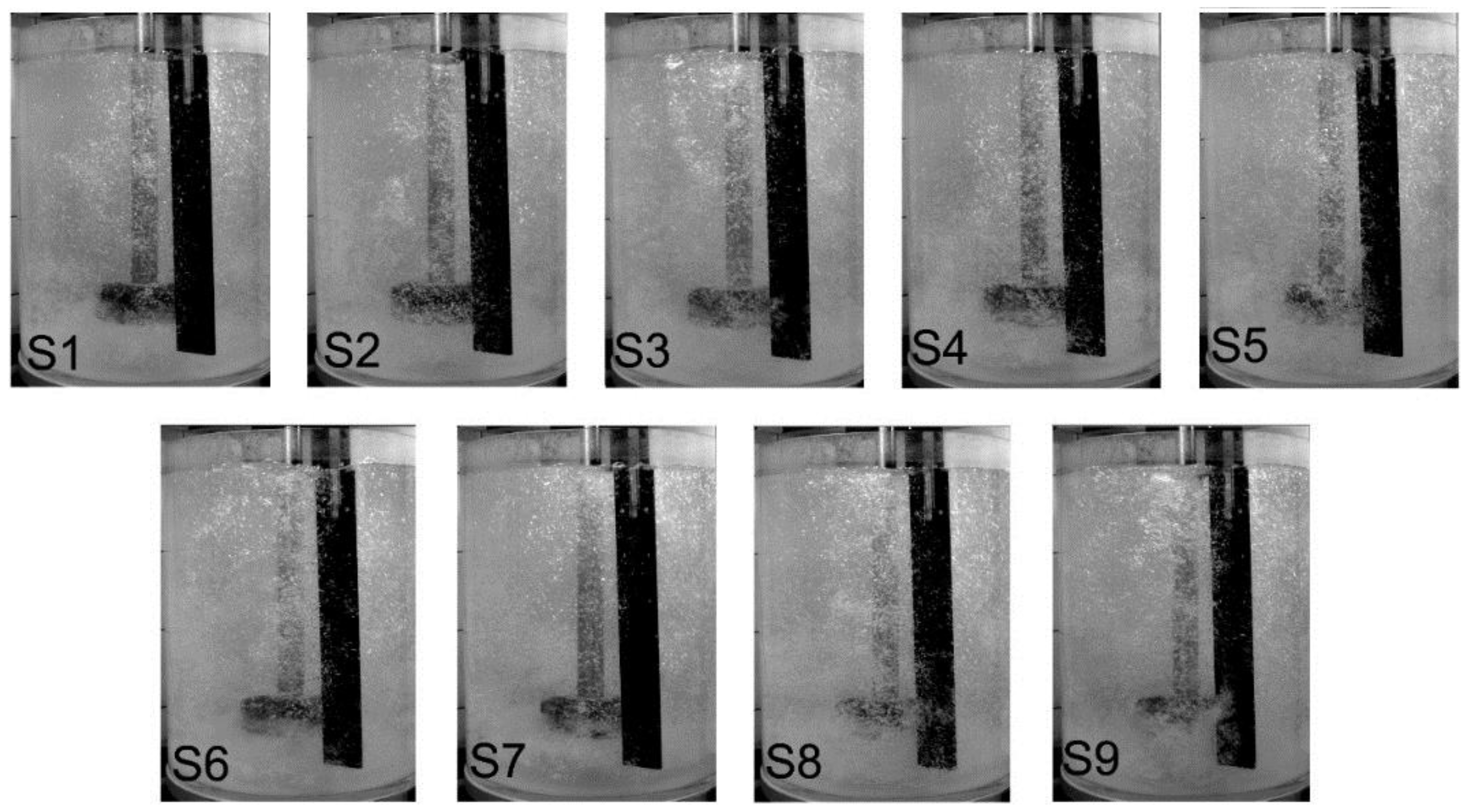
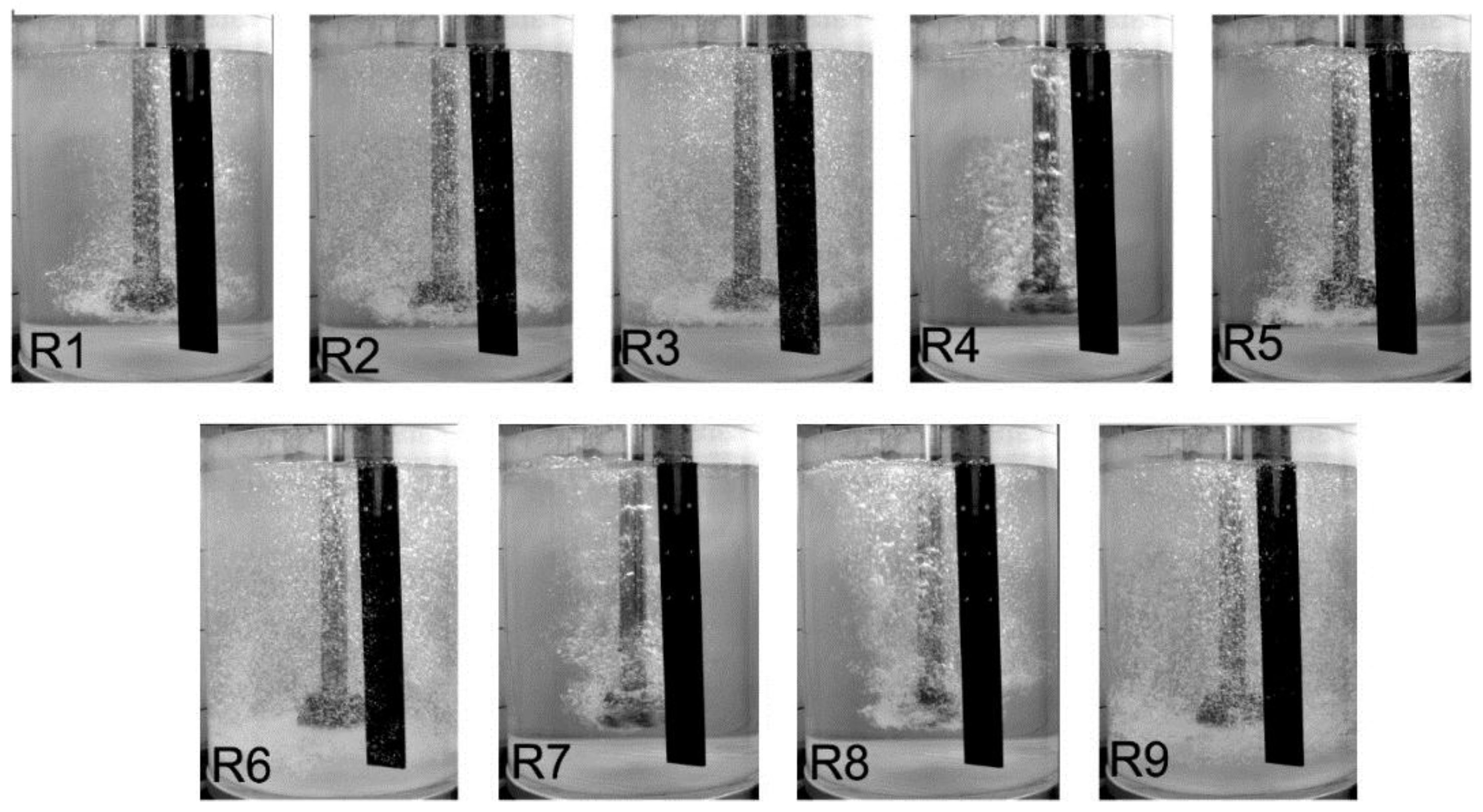
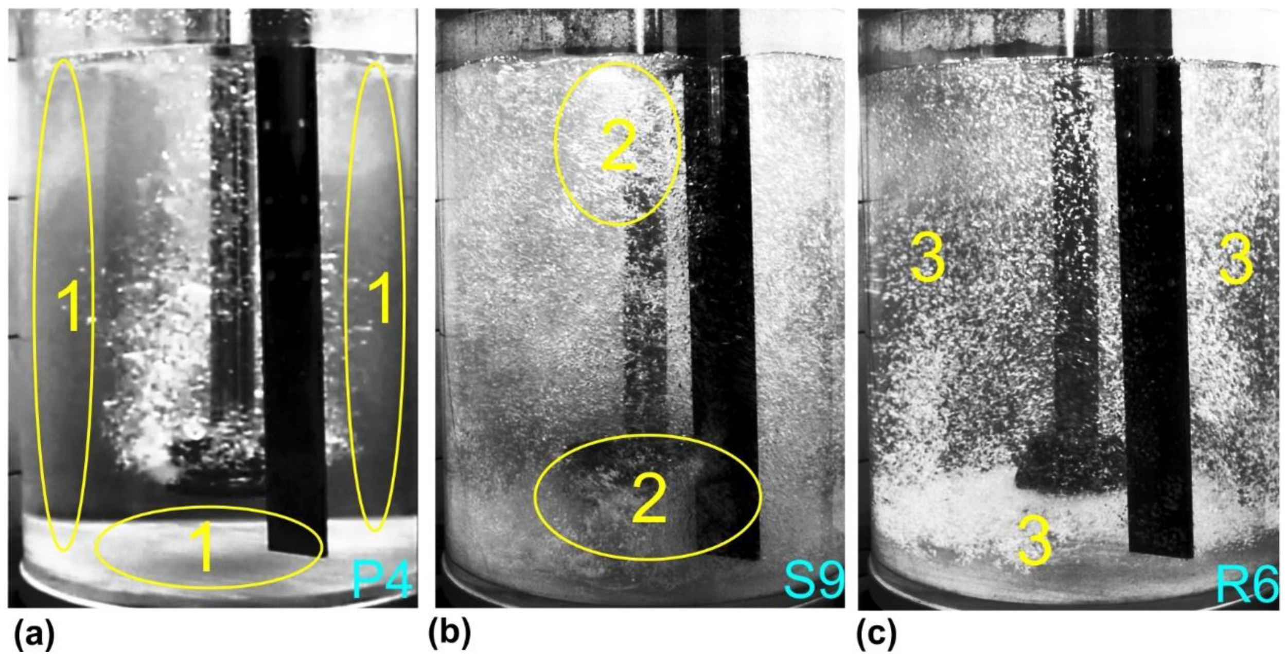
3.1. Visualisation Results
3.2. The Research of Oxygen Removal from Water
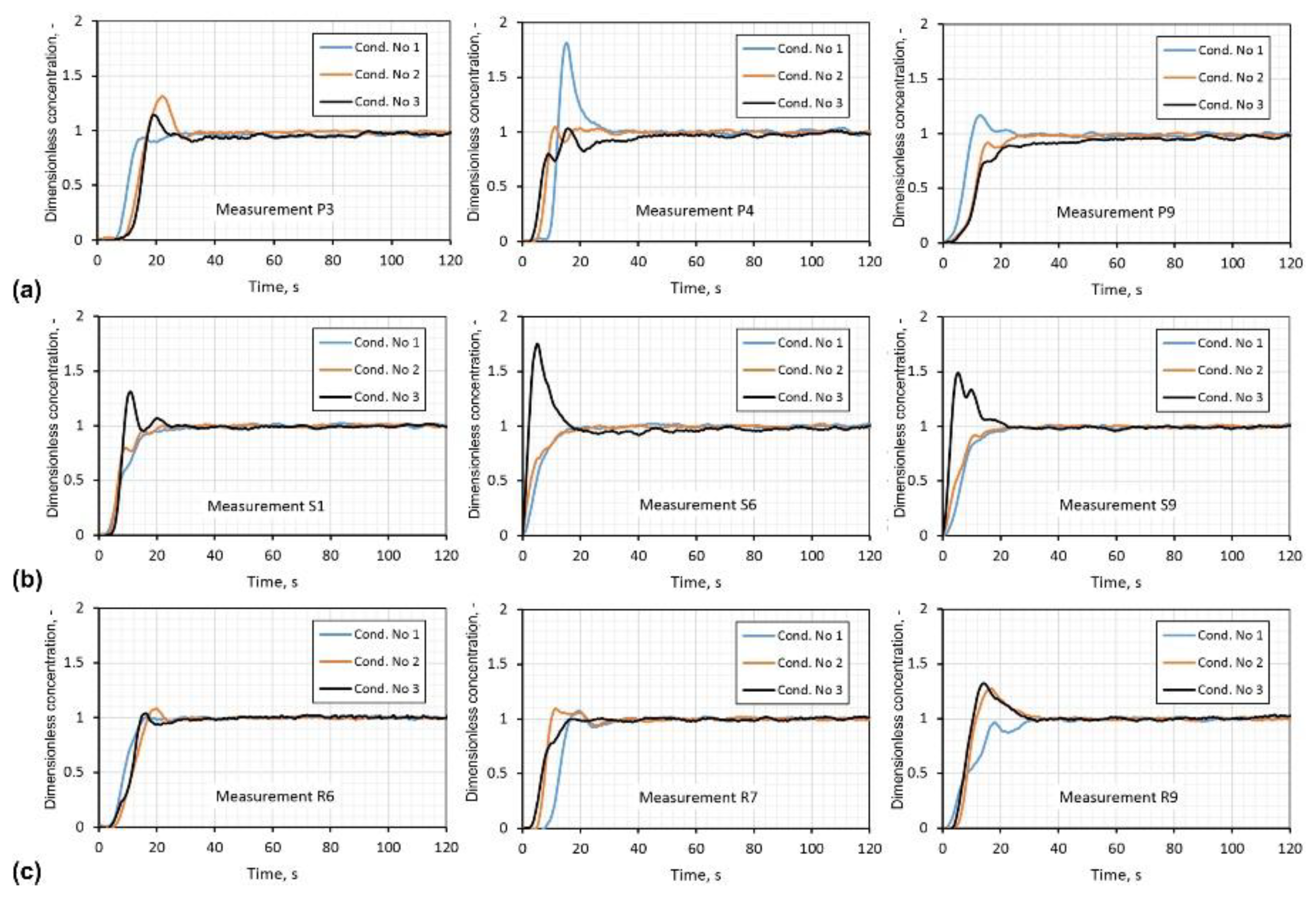
3.3. Determination of Residence Time Distribution(RTD) Curves
- Impeller A: the worst result (minimum dispersion)—Variant P4 and the best ones P3 and P9.
- Impeller B: the worst result (excessive dispersion)—Variant S9 and the best ones S1 and S6.
- Impeller C: the worst result (minimum dispersion)—Variant R7 and the best ones R6 and R9.
4. Conclusions
- Physical modelling is a helpful method for working out the new design rotary impeller and aids easy identification of the optimal processing parameters.
- The physical model of the refining reactor simulates the conditions prevailing in this reactor during refining process. The rates of gas bubble dispersion significantly influences the efficiency of the hydrogen removal process. Determining the optimal range of gas flow increases the efficiency of the purging process, which in turn reduces its costs.
- The information obtained from the dispersion patterns are dependent on observation and interpretation, and thus improper conclusions can be drawn.
- RTD curves, which are quantitative analysis, provide the information about mixing time of tracer with water, and based on such results the identification of processing parameters, such as flow rate of refining gas and rotary impeller speed, is possible. RTD curves do not give a direct and clear answer, but allow for a satisfactory estimation of the technological parameters and the operation of the reactor.
- Based on research of oxygen removal from water, as an analog of hydrogen desorption from aluminum, the essential information can be obtained about the process and processing parameters, and also about the time of refining.
- The new design impeller B had the best results in all applied methods, the best variants being 8.33 s−1 and 15 L·min−1. The next step of the research should now be to test the new design impeller under industrial conditions.
Author Contributions
Funding
Conflicts of Interest
References
- Saternus, M.; Botor, J. Physical model of aluminium refining process in URC-7000. Metalurgija 2009, 48, 175–179. [Google Scholar]
- Simensen, C.J.; Berg, G. A survey of inclusions in aluminium. Aluminium 1980, 56, 335–340. [Google Scholar]
- Gomez, E.R.; Zenit, R.; Rivera, C.G.; Trapaga, G.; Ramirez-Argaez, M.A. Physical modelling of the fluid flow in ladles of aluminium equipped with impeller and gas purging for degassing. Metall. Mater. Trans. B 2013, 44, 974–983. [Google Scholar] [CrossRef]
- Zhang, L.; Lv, X.; Torgerson, A.T.; Long, M. Removal of impurity elements from molten aluminum: A review. Miner. Process. Extr. Metll. Rev. 2011, 32, 150–228. [Google Scholar] [CrossRef]
- Taylor, M.B. Molten metal fluxing/treatment: How best achieve the desired quality requirements. Aluminium 2003, 79, 44–50. [Google Scholar]
- Waite, P. A Technical perspective on molten aluminum processing. In Light Metals, the Minerals, Metals and Materials Society; TMS: Seattle, DC, USA, 2002; pp. 841–848. [Google Scholar]
- Camacho-Martinez, J.L.; Ramirez-Argaez, M.A.; Juarez-Hernandez, A.; Gonzalez-Rivera, C.; Trapaga-Martinez, G. Novel degasification design for aluminum using an impeller degasification water physical model. Mater. Manuf. Process. 2012, 27, 556–560. [Google Scholar] [CrossRef]
- Li, J.H.; Hao, Q.T. Develop the degassing and purification equipment of molten aluminum alloys by rotary impeller. Foundry 2007, 56, 731–734. [Google Scholar]
- Saternus, M.; Botor, J. Refining process of aluminium conducted in continuous reactor—Physical model. Arch. Metall. Mater. 2010, 55, 465–475. [Google Scholar]
- Mancilla, E.; Cruz-Mendez, W.; Garduno, I.E.; Gonzalez-Rivera, C.; Ramirez-Argaez, M.A.; Ascanio, G. Comparison of the hydrodynamic performance of rotor-injector devices in a water physical model of an aluminum degassing ladle. Chem. Eng. Res. Des. 2017, 118, 158–169. [Google Scholar] [CrossRef]
- Oldshue, J.Y. Fluid Mixing Technology; Chemical Engineering McGraw-Hill Pub. Co.: New York, NY, USA, 1983; pp. 141–154. [Google Scholar]
- Hsi, R.; Tay, M.; Bukur, D.; Tatterson, G.; Morrison, G. Sound spectra of gas dispersion in an aerated agitated tank. Chem. Eng. J. 1985, 31, 153–161. [Google Scholar] [CrossRef]
- Warmoeskerken, M.M.C.G.; Smith, J.M. Flooding of disco turbines in gas-liquid dispersion: A new description of the phenomena. Chem. Eng. Sci. 1985, 40, 2063–2071. [Google Scholar] [CrossRef]
- Chen, J.J.J.; Zhao, J.C. Bubble distribution in a melt treatment water model. In Light Metals, the Minerals, Metals and Materials Society; TMS: Las Vegas, NV, USA, 1995; pp. 1227–1231. [Google Scholar]
- Zhao, J.C.; Chen, J.J.J. Gas line pressure fluctuation analysis of a gas-liquid reactor. J. Therm Sci. 2005, 14, 267–271. [Google Scholar]
- Chen, J.J.J.; Zhao, J.C.; Lacey, P.V.; Gray, T.N.H. Flow pattern in a melt treatment water model based on shaft power measurements. In Light Metals, the Minerals, Metals and Materials Society; TMS: New Orleans, LA, USA, 2001; pp. 1021–1025. [Google Scholar]
- Odenthal, H.J.; Bölling, R.; Pfeifer, H. Numerical and physical simulation of tundish fluid flow phenomena. Steel Res. 2003, 74, 44–55. [Google Scholar] [CrossRef]
- Saternus, M. Rafinacja Aluminium I Jego Stopów Przez Przedmuchiwanie Argonem; Politechnika Śląska: Gliwice, Poland, 2011; pp. 82–87. [Google Scholar]
- Evans, J.W.; Field, A.; Mittal, N. Measurements of bubble dispersion and other bubble parameters in a gas fluxing unit at Alcoa using a capacitance probe. In Light Metals, the Minerals, Metals and Materials Society; TMS: San Diego, CA, USA, 2003; pp. 909–913. [Google Scholar]
- Waz, E.; Carre, J.; Le Brun, P.; Jardy, A.; Xuereb, C.; Ablitzer, D. Physical modelling of the aluminum degassing process: Experimental and mathematical approaches. In Light Metals, the Minerals, Metals and Materials Society; TMS: San Diego, CA, USA, 2003; pp. 901–907. [Google Scholar]
- Camacho-Martinez, J.L.; Ramirez-Argaez, M.A.; Zenit-Camacho, R.; Juarez-Hernandez, A.; Barceinas-Sanchez, J.O.; Trapaga-Martinez, G. Physical modelling of an aluminum degassing operation with rotating impellers—A comparative hydrodynamic analysis. Mater. Manuf. Process. 2010, 25, 581–591. [Google Scholar] [CrossRef]
- Guofa, M.; Shouping, Q.; Xiangyu, L.; Jitai, N. Research on water simulation experiment of the rotating impeller degassing process. Mater. Sci. Eng. A 2009, 499, 195–199. [Google Scholar]
- Nilmani, M.; Thay, P.; Siemensen, C. A comparative study of impeller performance. In Light Metals, the Minerals, Metals and Materials Society; TMS: San Diego, CA, USA, 1992; pp. 939–946. [Google Scholar]
- Ohno, Y.; Hampton, D.T.; Moores, A.W. The GBF rotary system for total aluminum refining. In Light Metals, the Minerals, Metals and Materials Society; TMS: Denver, CA, USA, 1993; pp. 915–921. [Google Scholar]
- Nilmani, M.; Thay, P.K.; Simansen, C.J.; Irwin, D.W. Gas fluxing operation in aluminum melt refining laboratory and plant investigation. In Light Metals, the Minerals, Metals and Materials Society; TMS: Anaheim, CA, USA, 1990; pp. 747–754. [Google Scholar]
- Johansen, S.; Graadahl, S.; Tetlie, P.; Rasch, B.; Myrbostad, E. Can rotor based refining units be developed and optimized based on water model experiments? In Light Metals, the Minerals, Metals and Materials Society; TMS: San Antonio, TX, USA, 1998; pp. 805–810. [Google Scholar]
- Hernandez-Hernandez, M.; Camacho-Martinez, J.L.; Gonzalez-Rivera, C.; Ramirez-Argaez, M.A. Impeller design assisted by physical modelling and pilot plant trials. J. Mater. Process. Technol. 2016, 236, 1–8. [Google Scholar] [CrossRef]
- Chattopadhyay, K.; Isac, M.; Guthrie, R.I.L. Physcial and mathematical modelling of steelmaking tundish operations: A review of the last decade (1999–2009). ISIJ Int. 2010, 50, 331–348. [Google Scholar] [CrossRef]
- Saternus, M. Modelling research of hydrogen desorption from liquid aluminum and its alloys. Metalurgija 2011, 50, 257–260. [Google Scholar]
- Wen, C.Y.; Fan, L.T. Models for Flow Systems and Chemical Reactors; Chemical Processing and Engineering; Marcel Dekker, Inc.: New York, NY, USA, 1975; Volume 3, pp. 9–50. ISBN 0-8247-6346-7. [Google Scholar]
- Ferro, S.P.; Principe, R.J.; Goldschmit, M.B. A new approach to the analysis of vessel residence time distribution curves. Metall. Mater. Trans. B 2001, 32, 1185–1193. [Google Scholar] [CrossRef]
- Merder, T.; Pieprzyca, J.; Saternus, M. Analysis of residence tome distribution (RTD) curves for T-type tundish equipped in flow control devices—physical modelling. Metalurgija 2014, 53, 155–158. [Google Scholar]
- Kumar, A.; Koria, S.C.; Mazumdar, D. An assessment of fluid flow modeling and residence time distribution phenomena in steelmaking tundish systems. ISIJ Int. 2004, 44, 1334–1341. [Google Scholar] [CrossRef]
- Chattopadhyay, K.; Isac, M.; Gutrie, R.I.L. Modelling of non-isothermal melt flows in a four-strand delta shaped billet caster tundish validated by water model experiments. ISIJ Int. 2012, 52, 2026–2035. [Google Scholar] [CrossRef]
- Ramos-Gomez, E.; Zenit, R.; Gonzalez-Rivera, C.; Trapaga, G.; Ramirez-Argaez, M. Mathematical modelling of fluid flow in a water of an aluminum degassing ladle equipped with impeller-injector. Metall. Mater. Trans. B 2013, 44, 423–435. [Google Scholar] [CrossRef]
- Saternus, M. Influence of impeller shape on the gas bubbles dispersion in aluminum refining process. J. Achiev. Mater. Manuf. Eng. 2012, 55, 285–290. [Google Scholar]
- Chin, E.J.; Celik, C.; Hayes, P.; Bouchard, P.; Larouche, G. GIFS—A novel approach to in-line treatment of aluminum. In Light Metals, the Minerals, Metals and Materials Society; TMS: Anaheim, CA, USA, 1994; pp. 929–936. [Google Scholar]


| Characteristic Feature | Value | |||||||||
| Volume of the Tank | 230 L | |||||||||
| Velocity of Gas Bubble Flow (rotary impeller speed x distance from rotary impeller axis) | Impeller A | Impeller B | Impeller C | |||||||
| 0.375 m·s−1 | 0.475 m·s−1 | 0.350 m·s−1 | ||||||||
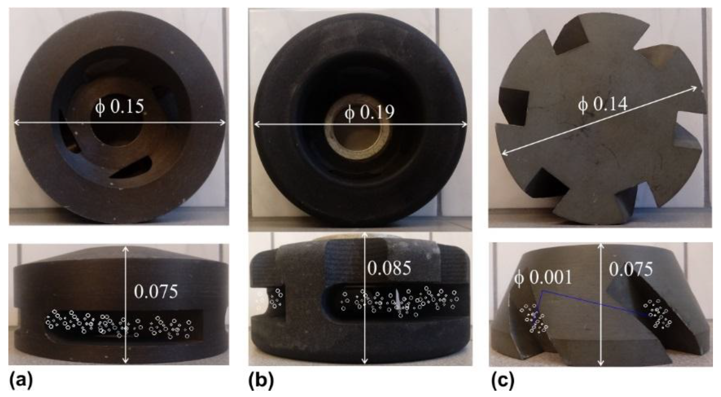
| Rotary Impeller Diameter | Impeller A | Impeller B | Impeller C | |||||||
| 0.15 m | 0.19 m | 0.14 m | ||||||||
| Criterial Numbers | ||||||||||
| Fluid | water | aluminum | ||||||||
| Temperature | 293 K | 973 K | ||||||||
| Dynamic Viscosity | 1005 Pa·s | 1000 Pa·s | ||||||||
| Surface Tension | 0.072 N·m−1 | 0.868 N·m−1 | ||||||||
| Density | 1000 kg·m−3 | 2700 kg·m−3 | ||||||||
| Reynold’s Number | Impeller A | Impeller B | Impeller C | Impeller A | Impeller B | Impeller C | ||||
| 56,250 | 90,250 | 49,000 | 151,875 | 243,675 | 132,300 | |||||
| Weber’s Number | 292.97 | 595.40 | 238.19 | 65.61 | 133.35 | 53.35 | ||||
| Froude’s Number | 0.095 | 0.121 | 0.089 | 0.095 | 0.121 | 0.089 | ||||
| Rotary Impeller A | ||||||||
| No. | Impeller Speed, s−1 | Gas Flow Rate, L·min−1 | No. | Impeller Speed, s−1 | Gas Flow Rate, L·min−1 | No. | Impeller Speed, s−1 | Gas Flow Rate, L·min−1 |
| P1 | 5.00 (300 rpm) | 10 | P2 | 6.66 (400 rpm) | 10 | P3 | 8.33 (500 rpm) | 10 |
| P4 | 15 | P5 | 15 | P6 | 15 | |||
| P7 | 20 | P8 | 20 | P9 | 20 | |||
| Rotary Impeller B | ||||||||
| No. | Impeller Speed, s−1 | Gas Flow Rate, L·min−1 | No. | Impeller Speed, s−1 | Gas Flow Rate, L·min−1 | No. | Impeller Speed, s-1 | Gas Flow Rate, L·min−1 |
| S1 | 5.00 | 10 | S2 | 6.66 | 10 | S3 | 8.33 | 10 |
| S4 | 15 | S5 | 15 | S6 | 15 | |||
| S7 | 20 | S8 | 20 | S9 | 20 | |||
| Rotary Impeller C | ||||||||
| No. | Impeller Speed, s−1 | Gas Flow Rate, L·min−1 | No. | Impeller Speed, s−1 | Gas Flow Rate, L·min−1 | No. | Impeller Speed, s-1 | Gas Flow Rate, L·min−1 |
| R1 | 5.00 | 10 | R2 | 6.66 | 10 | R3 | 8.33 | 10 |
| R4 | 15 | R5 | 15 | R6 | 15 | |||
| R7 | 20 | R8 | 20 | R9 | 20 | |||
| Flow Rate of Refining Gas, L·min−1 | Type of Dispersion | ||
|---|---|---|---|
| Rotary Impeller Speed, s−1 | |||
| 5.00 | 6.66 | 8.33 | |
| Impeller A | |||
| 10 | Minimum | Minimum | Uniform |
| 15 | Minimum | Minimum | Uniform |
| 20 | Minimum | Intimate | Uniform |
| Impeller B | |||
| 10 | Intimate | Uniform | Uniform |
| 15 | Intimate | Uniform | Uniform |
| 20 | Intimate | Uniform | Excessive uniform |
| Impeller C | |||
| 10 | Minimum | Intimate | Uniform |
| 15 | Minimum | Intimate | Uniform |
| 20 | Minimum | Intimate | Uniform |
| Type of Rotary Impeller | Variant | Efficiency of Gas Consumption E, ppm/liter |
|---|---|---|
| Rotary impeller A | P8 | 0.045 |
| Rotary impeller B | S7 | 0.065 |
| Rotary impeller C | R7 | 0.054 |
| Rotary Impeller A | Rotary Impeller B | Rotary Impeller C | |||
|---|---|---|---|---|---|
| Variants | Time, s | Variants | Time, s | Variants | Time, s |
| P1 | 1200 | S1 | 630 | R1 | 1020 |
| P2 | 1020 | S2 | 510 | R2 | 780 |
| P3 | 810 | S3 | 390 | R3 | 660 |
| P4 | 1050 | S4 | 480 | R4 | 930 |
| P5 | 870 | S5 | 390 | R5 | 720 |
| P6 | 720 | S6 | 300 | R6 | 570 |
| P7 | 930 | S7 | 420 | R7 | 1050 |
| P8 | 750 | S8 | 360 | R8 | 690 |
| P9 | 660 | S9 | 270 | R9 | 540 |
| Rotary Impeller A | Rotary Impeller B | Rotary Impeller C | |||
|---|---|---|---|---|---|
| Variants | Time, s | Variants | Time, s | Variants | Time, s |
| P1 | 32 | S1 | 23 | R1 | 35 |
| P2 | 35 | S2 | 25 | R2 | 33 |
| P3 | 30 | S3 | 28 | R3 | 25 |
| P4 | 45 | S4 | 35 | R4 | 32 |
| P5 | 40 | S5 | 25 | R5 | 25 |
| P6 | 32 | S6 | 18 | R6 | 23 |
| P7 | 31 | S7 | 30 | R7 | 30 |
| P8 | 30 | S8 | 24 | R8 | 25 |
| P9 | 30 | S9 | 23 | R9 | 30 |
© 2018 by the authors. Licensee MDPI, Basel, Switzerland. This article is an open access article distributed under the terms and conditions of the Creative Commons Attribution (CC BY) license (http://creativecommons.org/licenses/by/4.0/).
Share and Cite
Saternus, M.; Merder, T. Physical Modelling of Aluminum Refining Process Conducted in Batch Reactor with Rotary Impeller. Metals 2018, 8, 726. https://doi.org/10.3390/met8090726
Saternus M, Merder T. Physical Modelling of Aluminum Refining Process Conducted in Batch Reactor with Rotary Impeller. Metals. 2018; 8(9):726. https://doi.org/10.3390/met8090726
Chicago/Turabian StyleSaternus, Mariola, and Tomasz Merder. 2018. "Physical Modelling of Aluminum Refining Process Conducted in Batch Reactor with Rotary Impeller" Metals 8, no. 9: 726. https://doi.org/10.3390/met8090726
APA StyleSaternus, M., & Merder, T. (2018). Physical Modelling of Aluminum Refining Process Conducted in Batch Reactor with Rotary Impeller. Metals, 8(9), 726. https://doi.org/10.3390/met8090726