Modeling of Forming Limit Bands for Strain-Based Failure-Analysis of Ultra-High-Strength Steels ^†

Abstract

Increased passenger safety and emission control are two of the main driving forces in the automotive industry for the development of light weight constructions. For increased strength to weight ratio, ultra-high-strength steels (UHSSs) are used in car body structures. Prediction of failure in such sheet metals is of high significance in the simulation of car crashes to avoid additional costs and fatalities. However, a disadvantage of this class of metals is a pronounced scatter in their material properties due to e.g., the manufacturing processes. In this work, a robust numerical model is developed in order to take the scatter into account in the prediction of the failure in manganese boron steel (22MnB5). To this end, the underlying material properties which determine the shapes of forming limit curves (FLCs) are obtained from experiments. A modified Marciniak–Kuczynski model is applied to determine the failure limits. By using a statistical approach, the material scatter is quantified in terms of two limiting hardening relations. Finally, the numerical solution obtained from simulations is verified experimentally. By generation of the so called forming limit bands (FLBs), the dispersion of limit strains is captured within the bounds of forming limits instead of a single FLC. In this way, the FLBs separate the whole region into safe, necking and failed zones.

1. Introduction

The ability to assess with possibility of the forming limits of sheet metals is critical to avoid excessive thinning or localized necking. Forming limit curves (FLCs) are one of the highly recognized tools to foresee the failure in sheet metals. The concept of FLCs was first introduced by Keeler and Backofen for the tension-tension zone [1] and then further extended to the tension-compression zone by Goodwin [2]. Over the years, different experimental and numerical methods have been developed for the accurate determination of FLCs. The Nakazima out-of-plane test and the Marciniak in-plane test [3] are well-known approaches to experimentally generate FLCs. Besides experimental methods, numerical methods are used to investigate failure. Thereby, an important aspect is the strain localization during forming.

The available numerical methods can be divided into three main frameworks: the maximum force criteria, the Marciniak–Kuczynski (MK) models and the finite element (FE) methods. A basic necking criterion in a simple tension case was established by Considère [4] which was thereafter extended to biaxial stretching by Hill [5] and Swift [6]. Hill [5] expressed the localized necking as a discontinuity in the velocity and Swift [6] determined the instability condition in the plastic strain by expressing the yield stress as a function of the induced stress during the deformation of the diffused necking. Using Considère’s criteria, Hora and Tong [7] introduced ‘modified maximum force criteria’ (MMFC) taking into account the strain path after diffuse necking. These criteria have been used for the FLC determination under non-linear strain paths by Tong et al. [8,9]. The enhanced modified maximum force criterion (eMMFC) was introduced by Hora et al. [10] in 2008 considering the sheet thickness and the curvatures of the parts. Another approach to determine the necking is the bifurcation analysis that was discussed by Hill [11].

To overcome the drawback in the maximum force model, Marciniak and Kuczynski [3] developed a new model considering a pre-existing inhomogeneity in sheet metals. The instability begins along the inhomogeneity due to a gradual strain concentration under biaxial stretching. Strain-rate sensitivity and plane anisotropy have been further studied in the later works as additional influencing parameters [12]. Hutchinson and Neale [13] analyzed an imperfection sensitive MK model with $J_2$ (von Mises) flow theory for principal strain states varying from uniaxial to equibiaxial tension. In the work of Chan et al. [14], localized necking is studied for the negative minor strain region (uniaxial tension to plane strain). Additionally, the inhomogeneity oriented in zero-extension direction is analyzed in [5]. The complete FLCs of anisotropic rate sensitive materials with orthotropic symmetry have been predicted for linear and complex strain paths in the work of Rocha et al. [15].

The shape of the FLC depends on the constitutive equations used in the MK model. Yield criteria as well as the hardening relation can alter the limit strains. Different parameters influencing the FLCs are studied in the literature. Lian et al. [16] studied the variation of sheet metal stretchability by varying the shape of the yield surface. A yield function that describes the behavior of orthotropic sheet metals under full plane stress state was introduced by Barlat and Lian [17]. Cao et al. [18] implemented the general anisotropic yield criterion for localized thinning in the sheet metals into the MK model. Additional failure modes in sheet metals, namely ductile and shear failure criteria were included in CrachFEM (MATFEM, Munich, Germany). Eyckens et al. [19] extended the MK model to predict localized necking considering through-thickness shear (TTS) during the forming operations.

In addition to MK and MMFC methods, the finite element (FE)-based approach, introduced by Burford and Wagoner [20], is another way to determine FLCs. Boudeau and Gelin [21] worked on the prediction of localized necking in sheet metals during the forming processes through FE simulations. Combining a ductile fracture criterion with finite element simulations, Takuda et al. [22] predicted the limit strains under biaxial stretching. Different finite element methods for the prediction of FLCs can be found in [23,24,25,26].

Due to the scatter in material properties at different regions of sheet metals, it becomes difficult to precisely predict the failure strains by a single FLC. Hence, a scatter of material properties has to be determined and a band of FLCs needs to be defined. Janssens et al. [27] introduced the concept of forming limit bands (FLBs) to have a reliable estimate of the uncertainty of FLCs. Strano and Colosimo [28] extended it further with logistic regression analysis to generate FLBs from experimental data. Chen and Zhou [29] applied percent regression analysis to the curve fitting of experimental data of limit strains. The above-mentioned studies analyze the experimental data statistically to obtain FLBs. On the other hand, Banabic et al. [30] was one of the first to incorporate the concept of FLBs in a theoretical approach to improve the robustness. The MK model with BBC2003 [31] plasticity criterion and Hollomon and Voce hardening laws were used in the derivation of the limit strains. Later, Comsa et al. [32] generated an FLB using Hora’s MMFC model with the Hill’48 yield criterion and Swift’s hardening law.

The aim of this work is to develop a methodology to predict the failure in UHSS sheet metals during a car crash. To this end, first, the limit strains of a car component are evaluated experimentally. Then, the scatter of the material properties is considered by defining a range of hardening relations using curve fitting of the experimental data. A modified MK model with a simplification related to the zero extension angle is applied to form the bounds of the limit strains numerically. In this way, the bounds can capture the material scatter via a parametric study.

The present paper is structured as follows. In Section 2, a modified MK model with an inclined groove is presented based on the work of Rocha et al. [15]. To solve the discrete equations, an implicit integration method is employed in Section 3. The obtained results are validated in Section 4 based on the theory of the method. Furthermore, the experimental data and their post-processing are described in Section 5 to determine the material scatter. Based on a statistical analysis of the material scatter, the forming limit bands are generated and discussed in Section 6. Eventually, the results are summarized and conclusions are drawn.

2. Theory of Forming Limit Curve

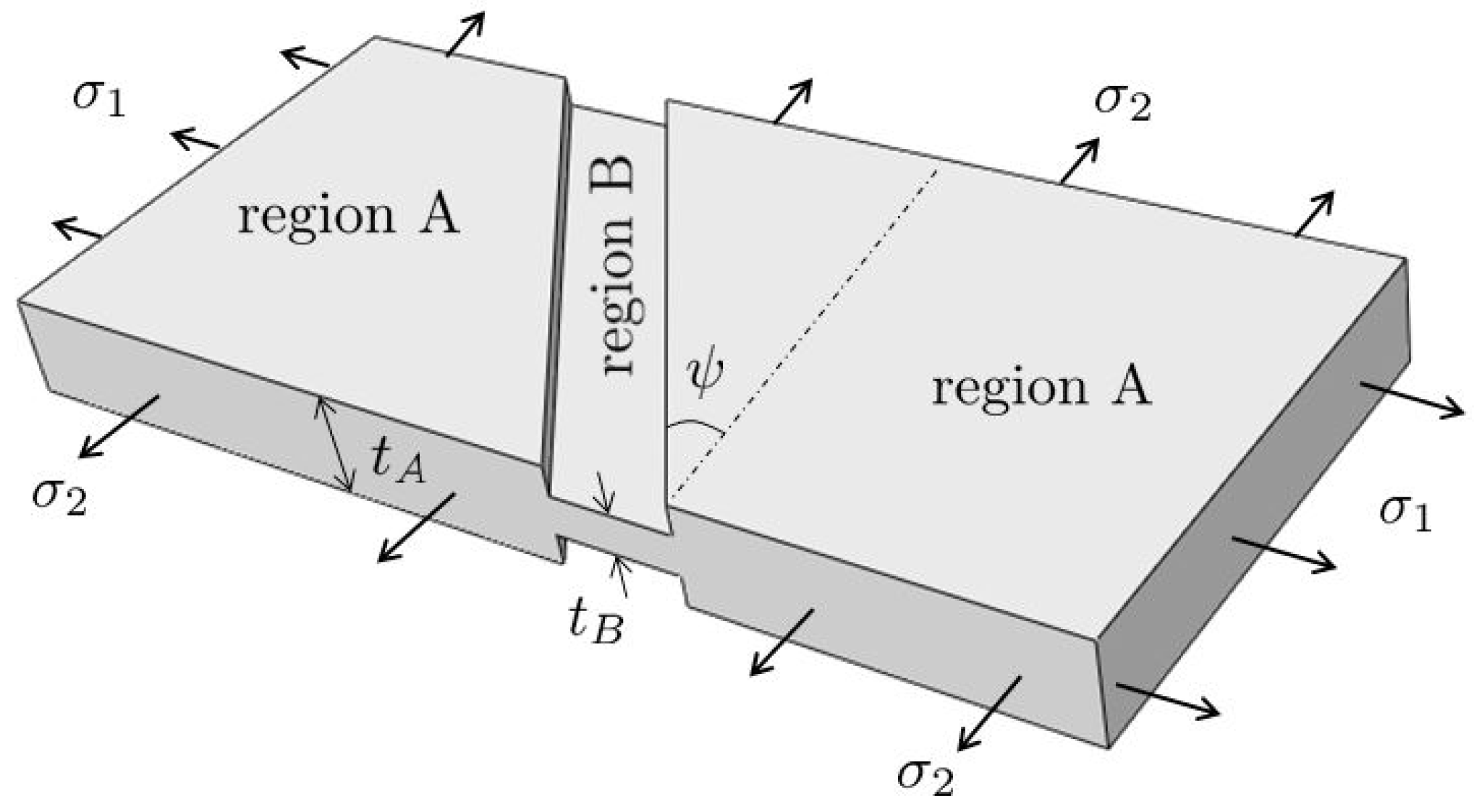
A sheet metal is subjected to biaxial stretching under a load given in terms of the principal stresses ${\sigma }_1$ and ${\sigma }_2$ as shown in Figure 1. The metal component has two regions with different thicknesses named as region A and region B. The groove, that is denoted as region B, is considered to make an angle $\psi$ with respect to the minor principal stress axis as shown in Figure 1. Although the thickness variation is smooth in reality, a sharp variation is considered to simplify the calculations. Due to its smaller thickness, region B will represent the necking region during the stretching operation.

Marciniak [3] introduced an inhomogeneity parameter expressed in terms of the ratio of the initial thicknesses of region B ($t_{0B}$) and A ($t_{0A}$). In the present work, it is denoted by $f_i$ and defined as

$$f_i=1-\frac{t_{0B}}{t_{0A}},$$

(1)

which implies that, when $f_i$ takes the value zero, the sheet is geometrically homogeneous. As stresses increase, the sheet metal undergoes different strain increments in non-necking and necking regions as indicated by subscripts A and B, respectively. The ratio of minor to major strain increments is assumed to remain constant within each load path. It is defined by

$$\gamma ={\displaystyle \frac{d{\epsilon }_{2A}}{d{\epsilon }_{1A}}}.$$

(2)

Strain and stress states of both regions (A and B) are monitored separately. In this way, one can define plastic instability as the increment of the equivalent plastic strain in region B becomes considerably greater than that of region A. The plastic instability indicator $\beta$ is expressed as the ratio between the equivalent plastic strain increments in region A ($d{\overline{\epsilon }}_A$) and region B ($d{\overline{\epsilon }}_B$) [34]:

$$\beta ={\displaystyle \frac{d{\overline{\epsilon }}_A}{d{\overline{\epsilon }}_B}}.$$

(3)

In practice, the value of $\beta$ is considered as 0.1 to indicate the loss of stability. The model is derived for an anisotropic material with an orthotropic symmetry. The classical Lankford coefficients $R_0$, $R_{45}$ and $R_{90}$ are considered as measures of anisotropy with respect to different directions of in-plane loading (angles $0^{\circ }$, ${45}^{\circ }$ and ${90}^{\circ }$ with respect to the rolling direction). Additionally, planar anisotropy is assumed and characterized by a time-independent average R-value defined by

$$\overline{R}={\displaystyle \frac{R_0+2R_{45}+R_{90}}{4}}.$$

(4)

In the case of isotropic material, the value of $\overline{R}$ becomes equal to unity. We define

$$\alpha ={\sigma }_2/{\sigma }_1$$

(5)

as the ratio of stresses in the principal directions, namely ${\sigma }_1$ and ${\sigma }_2$ [15]. The Hill’48 yield criterion is used in combination with an associative flow rule and Swift hardening relation. Hill’s criterion for in plane stress conditions is expressed as

$$2f={\overline{\sigma }}^2=F{\sigma }_{yy}^2+G{\sigma }_{xx}^2+H{({\sigma }_{xx}-{\sigma }_{yy})}^2+2P{\sigma }_{xy}^2,$$

(6)

where $\overline{\sigma }$ denotes the equivalent stress and F, G, H, and P are functions of the Lankford coefficients. Thus, they are material specific constants. The reader is referred to the Appendix A for more information about these constants. In the following, strain rate dependent stress relation similar to the classical MK model [12] is defined:

$$\overline{\sigma }=C_1{\left({\epsilon }_0+\overline{\epsilon }\right)}^n{\dot{\overline{\epsilon }}}^m.$$

(7)

In the latter relation, $C_1$ is a strength coefficient and ${\epsilon }_0$ denotes the initial yield strain. In addition, $\overline{\epsilon }$ represents the equivalent plastic strain with n as isotropic hardening exponent. Furthermore, m is the strain rate exponent. The associated flow rule is given by

$$d{\epsilon }_{ij}=d{\lambda }^{\prime }{\displaystyle \frac{\partial f}{\partial {\sigma }_{ij}}},$$

(8)

where $d{\lambda }^{\prime }$ is the hardening parameter being expressed as

$$d{\lambda }^{\prime }=d\overline{\epsilon }/\overline{\sigma }$$

and ${\epsilon }_{ij}$ are logarithmic strain components. Similar to the classical MK model, the incompressibility condition is given by

$$d{\epsilon }_{1A}+d{\epsilon }_{2A}+d{\epsilon }_{3A}=0.$$

(9)

Considering the strain in thickness direction, the sheet thickness can be written as

$$t_A=t_{0A}{e}^{{\epsilon }_{3A}},t_B=t_{0B}{e}^{{\epsilon }_{3B}}.$$

(10)

The force equilibrium conditions are given by

$${\sigma }_A^{nn}{t}_A={\sigma }_B^{nn}{t}_B,$$

(11)

$${\sigma }_A^{nt}{t}_A={\sigma }_B^{nt}{t}_B,$$

(12)

where n and t (in Equations (11) and (12)) denote the normal and tangential direction with respect to the inhomogeneity, respectively. The compatibility condition across the discontinuity is defined by

$$d{\epsilon }_A^{tt}=d{\epsilon }_B^{tt}.$$

(13)

First, the force equilibrium in normal direction (Equation (11)) is divided by $\overline{\sigma }$. Next, by using Equations (1) and (7) in (11) and upon simplification, the following relation is derived

$${\displaystyle \frac{co{s}^2\psi +\alpha si{n}^2\psi }{\sqrt{1+(F+H){\alpha }^2-2H\alpha }}}=(1-f_i)exp({\epsilon }_{3B}-{\epsilon }_{3A}){\left({\displaystyle \frac{{\epsilon }_0+{\overline{\epsilon }}_B}{{\epsilon }_0+{\overline{\epsilon }}_A}}\right)}^n{\left({\displaystyle \frac{d{\overline{\epsilon }}_B}{d{\overline{\epsilon }}_A}}\right)}^m\sqrt{{\displaystyle \frac{B_1{(d{\overline{\epsilon }}_A/d{\overline{\epsilon }}_B)}^2+B_2}{B_3}}}.$$

(14)

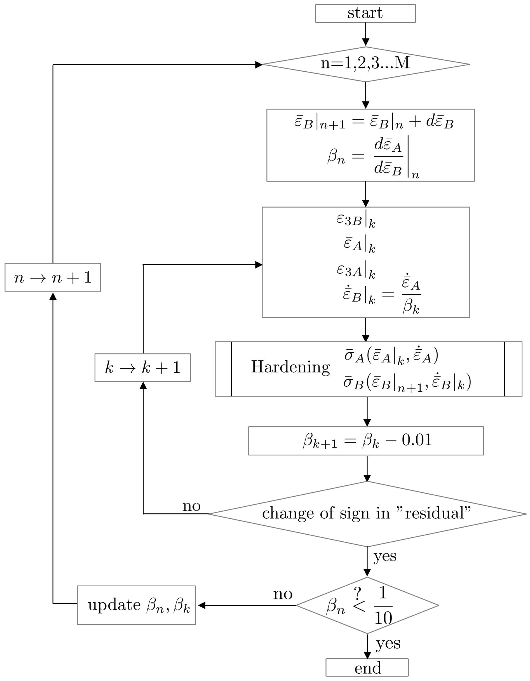
Equation (14) represents the residual in the algorithm described in Section 3. Strain increments in the third direction for regions A and B are derived by the application of compatibility and incompressiblity conditions

$$d{\epsilon }_{3A}=-{\displaystyle \frac{G+F\alpha }{\sqrt{1+(F+H){\alpha }^2-2H\alpha }}}d{\overline{\epsilon }}_A,$$

(15)

$$d{\epsilon }_{3B}=-\left[H_6\sqrt{{\displaystyle \frac{B_1{(d{\overline{\epsilon }}_A/d{\overline{\epsilon }}_B)}^2+B_2}{B_3}}}+H_7\left({\displaystyle \frac{d{\overline{\epsilon }}_A}{d{\overline{\epsilon }}_B}}\right)\right]d{\overline{\epsilon }}_B,$$

(16)

where $B_1$, $B_2$, $B_3$, $H_6$ and $H_7$ are functions of $R_0,R_{45},R_{90},\psi$ and $\alpha$. For a detailed derivation the reader is referred to the Appendix A and to Rocha et al. [15].

The above mentioned mathematical model is capable of evaluating the limit strain for both positive and negative minor strains ${\epsilon }_2$. There are four different fundamental strain paths, i.e., uniaxial tension, plane strain, biaxial and equibiaxial tension. The relation between the stress ratio $\alpha$ and the strain ratio $\gamma$ for an isotropic material is given by [14,34]

$$\alpha ={\displaystyle \frac{2\gamma +1}{2+\gamma }}.$$

(17)

Table 1. Incremental strain and stress ratios for four different load paths.

-	Uniaxial	Plane Strain	Biaxial	Equibiaxial
$\gamma$	$-0.5$	0	0.5	1
$\alpha$	0	0.5	0.8	1

shows the corresponding values of $\alpha$ calculated from Equation (17).

In the tension-compression quarter of the FLC, the limit strains depend on the (initial) orientation of the groove. Therefore, an arbitrary angle $\psi$ between the direction of the imperfection and the direction of the principal minor stresses is considered as described in Figure 1. As FLCs represent the maximum allowable strains, the minimum limit strains of all the possible orientations of the groove are to be identified. Upon implementing the rotation of angle from $0^{\circ }$ to ${45}^{\circ }$ to evaluate the minimum strain, the computational cost of the algorithm is increased. This can be simplified by using the concept of zero extension direction provided by Hill’s theory [5]. As predicted by this theory, if the imperfection is oriented along the zero extension direction, there will be a substantial difference in the limit strain compared to that of $\psi =0^{\circ }$ [14].

According to the theory of Hill [5], localized necking occurs along the direction of zero extension, which is determined by [35]

$${\psi }^{\ast }=ta{n}^{-1}\sqrt{-\gamma }.$$

(18)

The zero extension angle in case of uniaxial tension for planar isotropic material is found to be ${\psi }^{\ast }={35.3}^{\circ }$. From Chan et al. [14], the calculated limit strains using the zero extension direction are within $2\%$ of the limit strains calculated based on the aforementioned rotation of the imperfection. Thus, for the purpose of simplification and faster computation the angular orientation of the discontinuity is set to the zero extension angle, which is investigated later in this work.

3. Numerical Solution and Algorithm

The numerical solution is performed by means of an implicit integration method. To this end, the algorithm is implemented using two loops in FORTRAN similar to that of Werner [34]. Here, the value of $\beta$ is unknown and evaluated as a function of the equivalent plastic strain in the necking region. The computation continues until $\beta$ reaches a critical value of $0.1$. The iterative technique used to solve for $\beta$ is shown in Figure 2. In the outer loop (n loop), ${\overline{\epsilon }}_B$ is increased by a constant increment $d{\overline{\epsilon }}_B$. In this work, $d{\overline{\epsilon }}_B$ is set to $0.001$ (refer to Figure 3). This is given by

$${\overline{\epsilon }}_B{{|}_{n+1}={\overline{\epsilon }}_B|}_n+d{\overline{\epsilon }}_B.$$

(19)

The inner loop (k loop) is running for a maximum number of 100 times by varying $\beta$ from 1 to 0 in steps of 0.01. This loop terminates when the sign of the residual represented in Equation (14) changes. The plastic strain $d{\overline{\epsilon }}_A$ in the non-necking region is calculated by arithmetic averaging of two consecutive $\beta$ values within the n loop (refer to Equation (22)). To start the algorithm ${\overline{\epsilon }}_A$, ${\overline{\epsilon }}_B$, ${\epsilon }_{3A}$, ${\epsilon }_{3B}$ as well as $d{\overline{\epsilon }}_A/d{\overline{\epsilon }}_B=\beta$ must be initialized. Here, the initial conditions as set as follows:

$$\begin{array}{c}\hfill \begin{array}{cc}\hfill {\overline{\epsilon }}_A{|}_0& ={\overline{\epsilon }}_B{|}_0=0,\hfill \\ \hfill {\epsilon }_{3A}{|}_0& ={\epsilon }_{3B}{|}_0=0\mathrm{and}\hfill \\ \hfill {\beta }_0& =1.\hfill \end{array}\end{array}$$

(20)

The inhomogeneity parameter $f_i$ is manually input. In every k loop, first $d{\epsilon }_{3B}$ is calculated using Equation (16) since the values of $d{\overline{\epsilon }}_A$, $d{\overline{\epsilon }}_B$, $\alpha$ and $\overline{R}$ are already known. In the next step, ${\epsilon }_{3B}$ is computed using the equation

$${\epsilon }_{3B}{|}_k={\epsilon }_{3B}{{|}_n+d{\epsilon }_{3B}|}_k,$$

(21)

where the variable ${\epsilon }_{3B}{|}_n$ is already initialized. Next, $d{\overline{\epsilon }}_A{|}_k$ is calculated using the arithmetic averaging:

$$d{\overline{\epsilon }}_A{|}_k=0.5({\beta }_n+{\beta }_k)d{\overline{\epsilon }}_B.$$

(22)

Having initialized $\beta$ and ${\overline{\epsilon }}_A{|}_n$, we determine ${\overline{\epsilon }}_A{|}_k$ using the relation

$${\overline{\epsilon }}_A{|}_k={\overline{\epsilon }}_A{{|}_n+d{\overline{\epsilon }}_A|}_k.$$

(23)

Next, ${\epsilon }_{3A}$ is calculated in analogy to the previous equation by using $d{\epsilon }_{3A}$ from Equation (15)

$${\epsilon }_{3A}{|}_k={\epsilon }_{3A}{{|}_n+d{\epsilon }_{3A}|}_k.$$

(24)

Hardening relations ${\overline{\sigma }}_A$ and ${\overline{\sigma }}_B$ are computed using ${\overline{\epsilon }}_A{|}_k$, ${\overline{\epsilon }}_B{|}_{n+1}$ and the expression

$${\dot{\overline{\epsilon }}}_B{|}_k={\dot{\overline{\epsilon }}}_A/{\beta }_k$$

which is obtained by

$${\displaystyle \frac{{\dot{\overline{\epsilon }}}_B}{{\dot{\overline{\epsilon }}}_A}}={\displaystyle \frac{d{\overline{\epsilon }}_B}{dt}}{\displaystyle \frac{dt}{d{\overline{\epsilon }}_A}}.$$

(25)

For different load cases, the value of $\alpha$ is considered in Table 1. Other load cases are set by defining the value of $\alpha$ between 0 to 1.

In this work, hardening relations are fitted to experiments and implemented in the code.

4. Verification

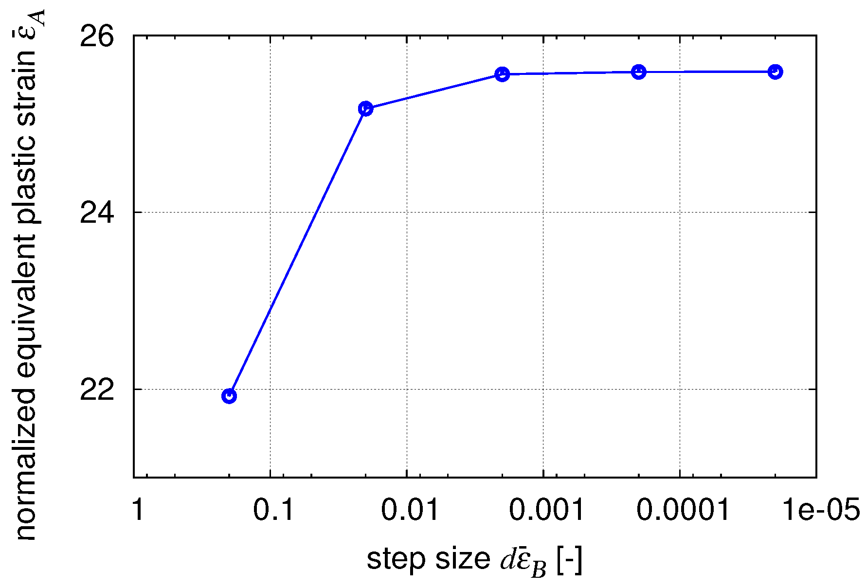
To verify the convergence properties of the solution method, different step sizes of $d{\overline{\epsilon }}_B$ are set ranging from $2\times {10}^{-5}$ to $0.2$. Without changing the other parameters such as hardening relations, anisotropy etc., the limit strains in region A are evaluated. It is clearly seen in Figure 3 that the limit strains (${\overline{\epsilon }}_A$) are close to convergence as $d{\overline{\epsilon }}_B$ approaches $0.002$. Therefore, the step size is set to $0.001$. Henceforth, all strains and stress measures are normalized to the mean ultimate tensile strength ($R_m$) and the mean uniform strain of entire samples, respectively.

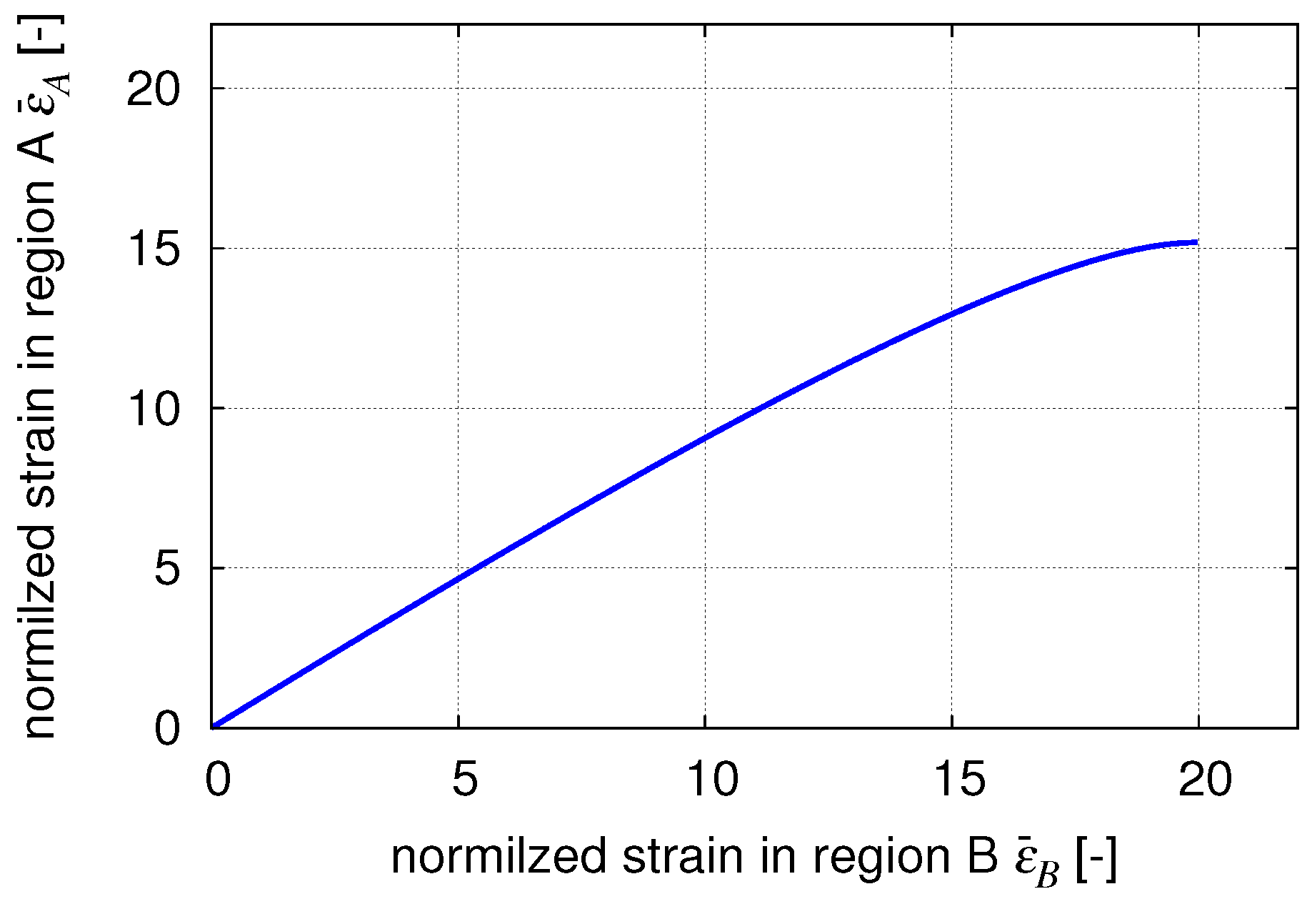
To verify the results, a hardening relation for a manganese boron steel (22MnB5) is applied. In addition, the material is assumed to be isotropic in this work. Nonetheless, due to the confidentiality of the project the parameters of the hardening relation (Equation (7)) are not explicitly revealed. In Figure 4, the evolution of the equivalent plastic strain (${\overline{\epsilon }}_A$) in the non-necking region is plotted against its counterpart (${\overline{\epsilon }}_B$) in the necking region. Initially, the slope of the curve is found to be approximately 1, since both regions are undergoing the same strain. At some point, the strain in region B starts to grow significantly faster than the one in region A. This is due to the localized necking in region B since it has a smaller cross-section. The difference between the strains in regions A and B is captured vividly for normalized strains in region B greater than 10. 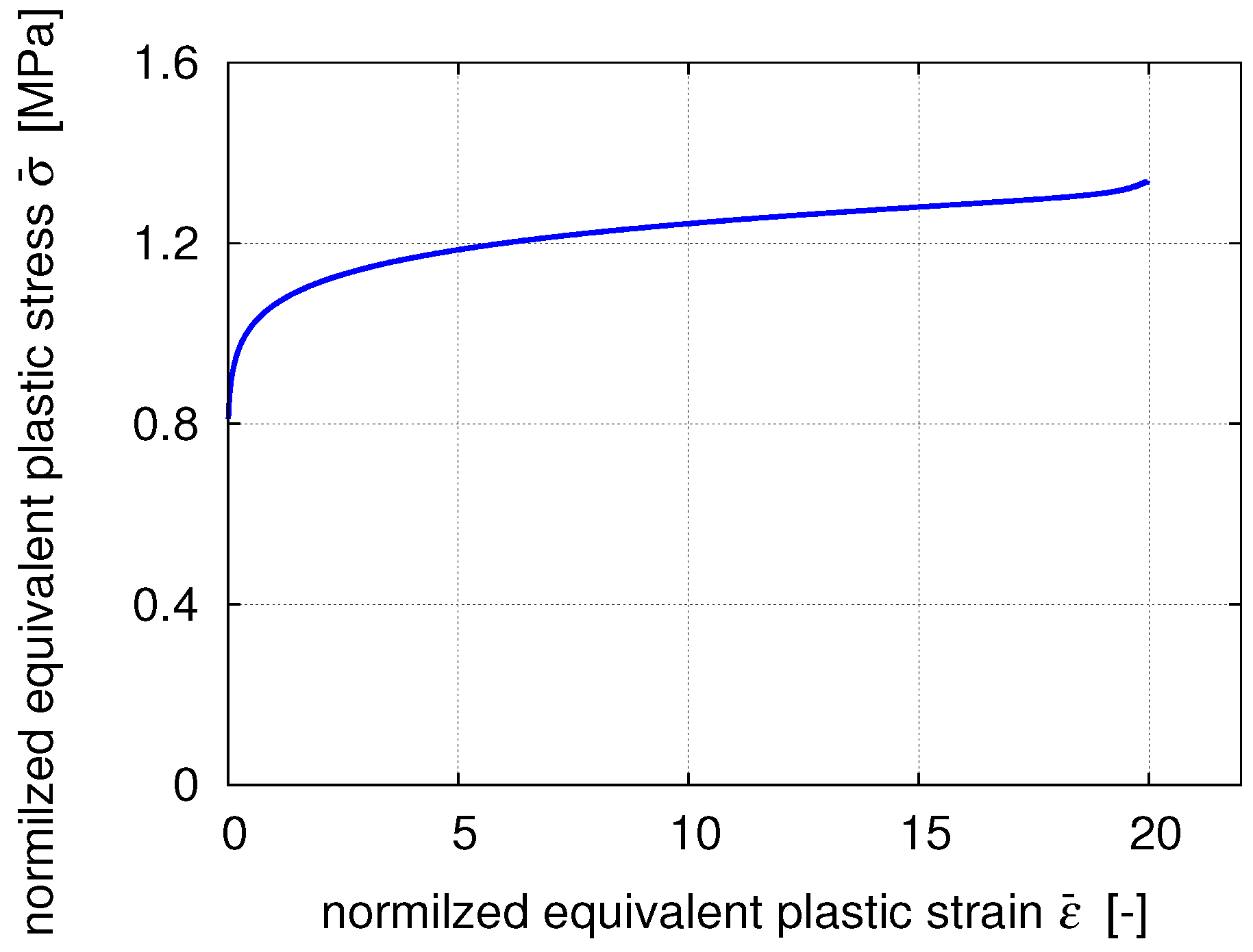In addition, the stress-strain curve in region B is plotted in Figure 5 for sheet metals subjected to equibiaxial tension. This plot captures the implemented hardening relation and represents the material behavior in the non-linear regime.

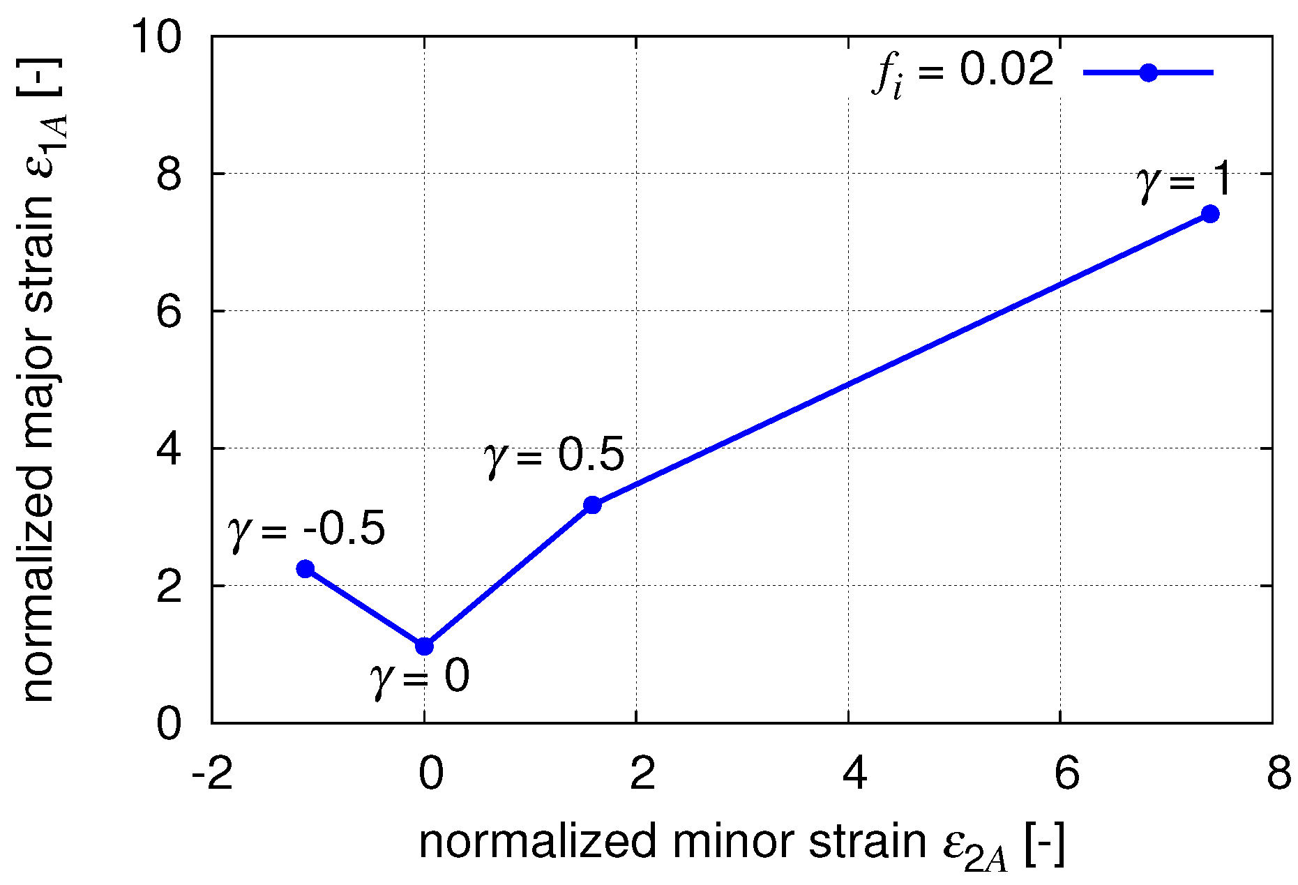
The maximum admissible strains that the material can withstand before the onset of necking are shown in Figure 6. Localized necking is evaluated by considering a constant predefined value of strain ratio $\gamma$ during the deformation process. The entire curve is obtained by varying $\gamma$ from $-0.5$ to 1 in steps of $0.5$.

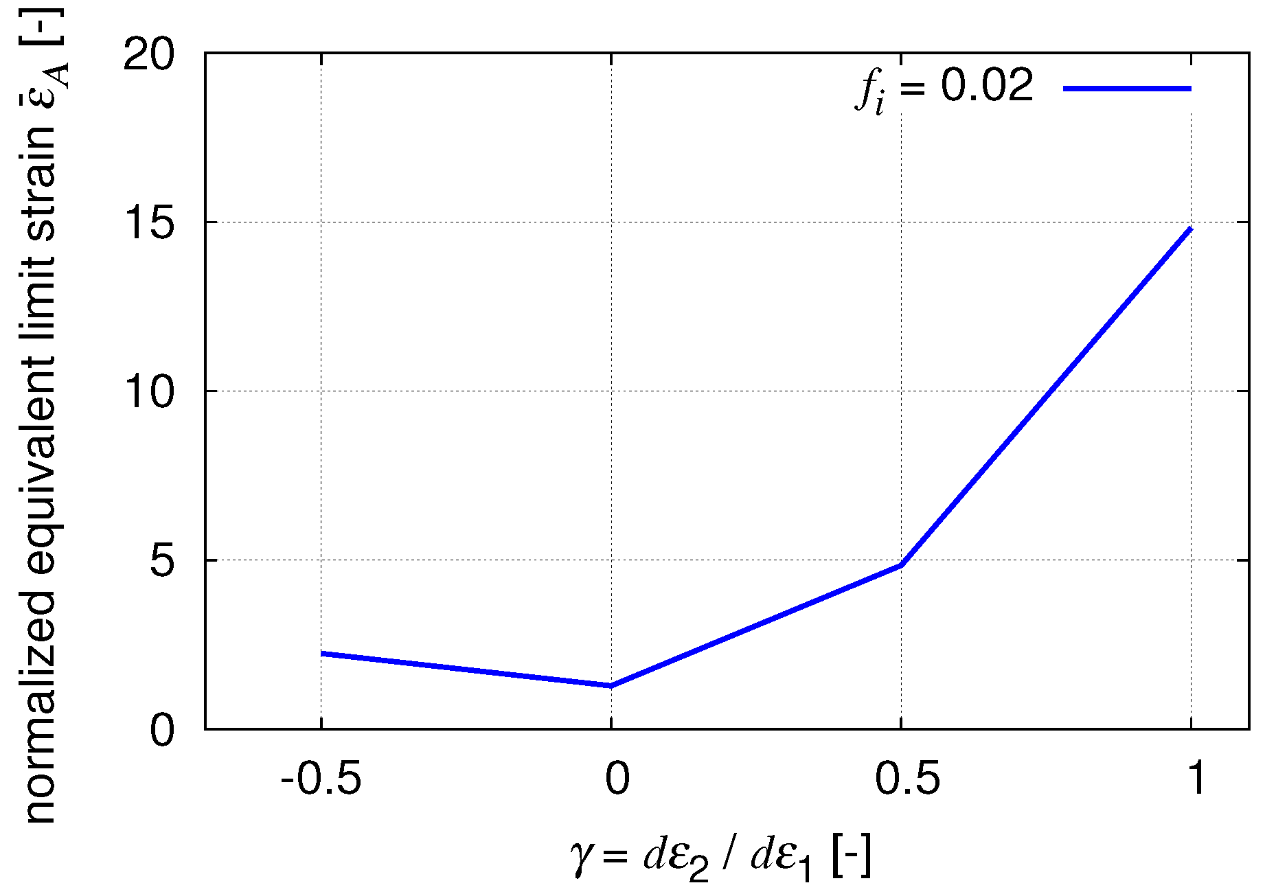
The limit strains can also be related to the equivalent plastic strain as shown in Figure 7. In this figure, the load path dependence of the limit strains is clearly evident. For instance, it is noticeable that sheet metals can deform to a higher extent under equibiaxial tension compared to uniaxial tension. Moreover, the choice of the inhomogeneity parameter $f_i$ plays a crucial role in the position of an FLC. The higher the inhomogeneity parameter, the lower is the entire FLC. In this section, it is set to $0.02$ for all loading paths. A detailed investigation of the aforementioned parameter is discussed in Section 6.

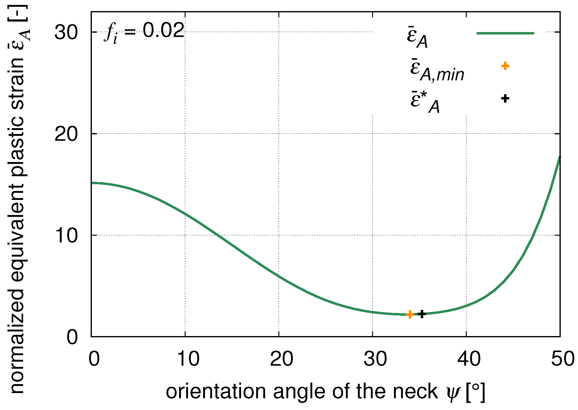
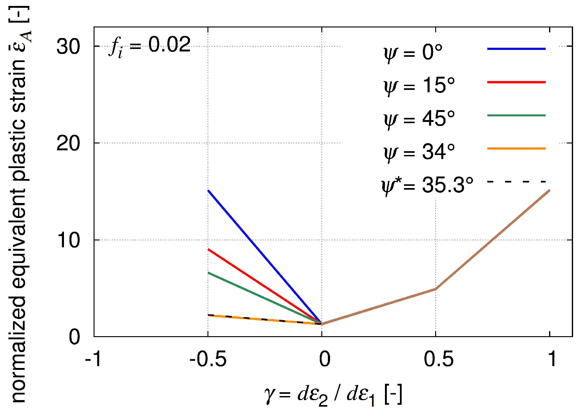
The effect of the angular orientation of the inhomogeneity in the tension-compression regime is studied in Figure 8 and Figure 9. It is evident that the choice of $\psi =0^{\circ }$ leads to an overestimation of the limit strains as depicted in Figure 9. This signifies the application of the angled groove for the tension-compression loading regime of the FLC. Furthermore, to compare the strains for any arbitrary orientation of the angle with that of the zero extension angle (${\overline{\epsilon }}_A^{\ast }$) from [35], an interval of $0^{\circ }$–${50}^{\circ }$ is considered, due to the symmetric influence of the orientation of the groove. The minimum equivalent strain (${\overline{\epsilon }}_{A,min}$) is found at the angle ${34}^{\circ }$. On the other hand, the zero extension angle obtained here is equal to ${35.3}^{\circ }$ which yields approximately the same limit strain ${\overline{\epsilon }}_A^{\ast }$ as ${\overline{\epsilon }}_{A,min}$. This is seen clearly in Figure 9, where both strains are mostly equal.

5. Experiments

Once the numerical method is verified, it needs to be validated with the experimental data. To obtain a precise and accurate strain measurement, a digital image correlation (DIC) measurement system was employed in the experiments. This method is able to display full-field strain measurement in the localized necking region. Simultaneous evaluation of the major and minor strains at any point makes it suitable for FLC related applications. In this project, the non-contact and material independent measurement system ARAMIS (v6.3, GOM, Braunschweig, Germany) is used for strain measurements. The stress values are obtained from the universal testing machine Zwick Z100 (Zwick Roell, Ulm, Germany).

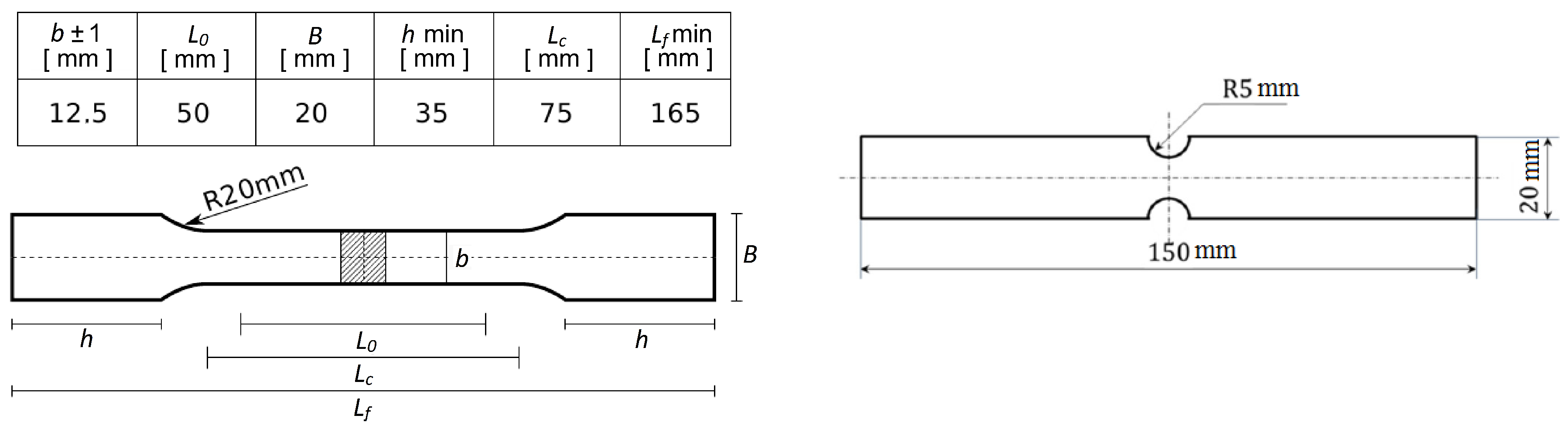
The experiments are performed by extracting samples from structural components of a car. These body parts are formed/stamped steels which are later heat treated to yield similar material properties like those of car components. To record the scattered material properties, samples from ten different batches are considered. Each batch consists of six components and each component delivers 12 test samples (extracted from six different regions). A total of 720 samples are extracted for two different test categories, namely notched and A50 specimens (see Figure 10).

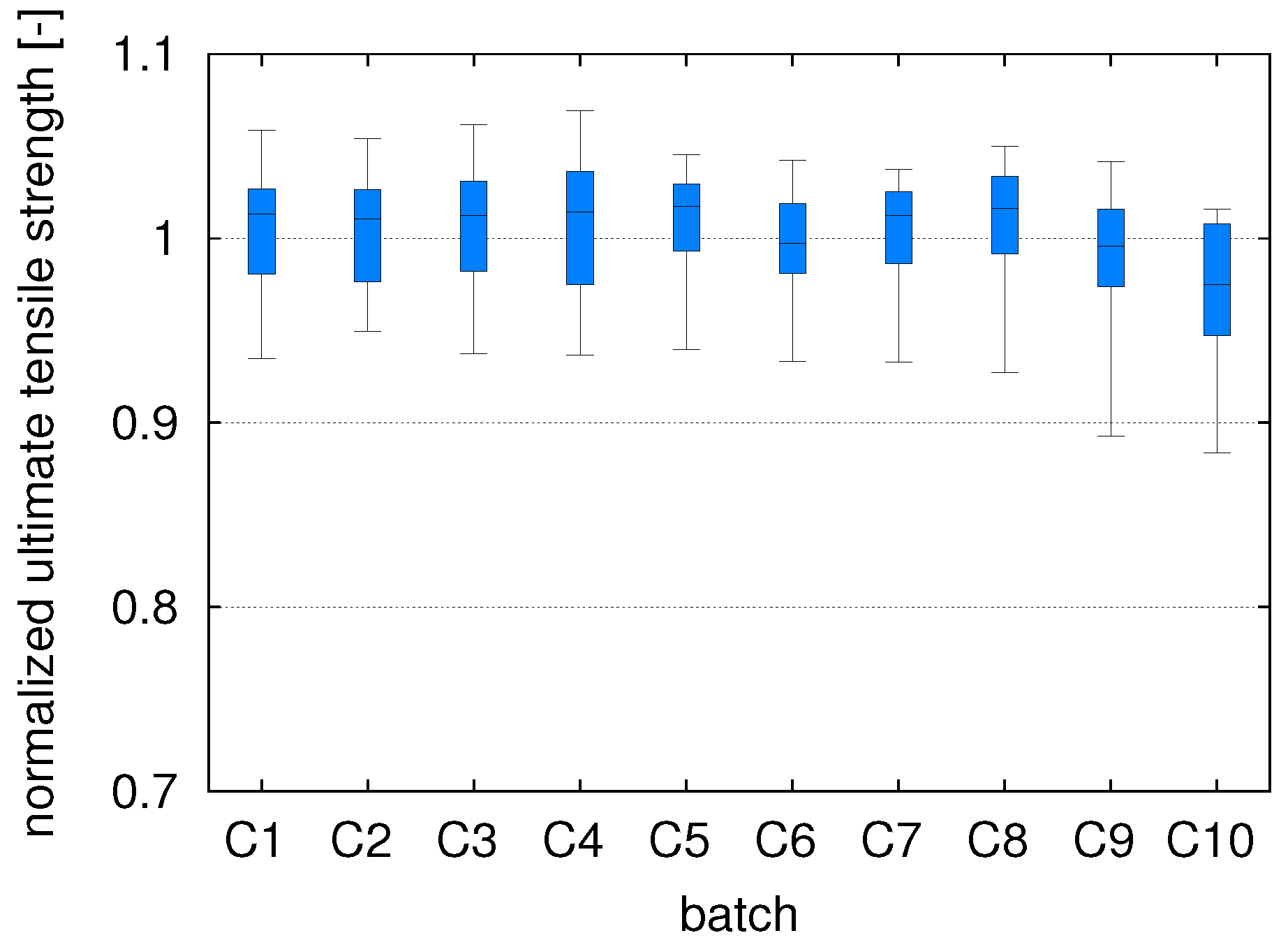
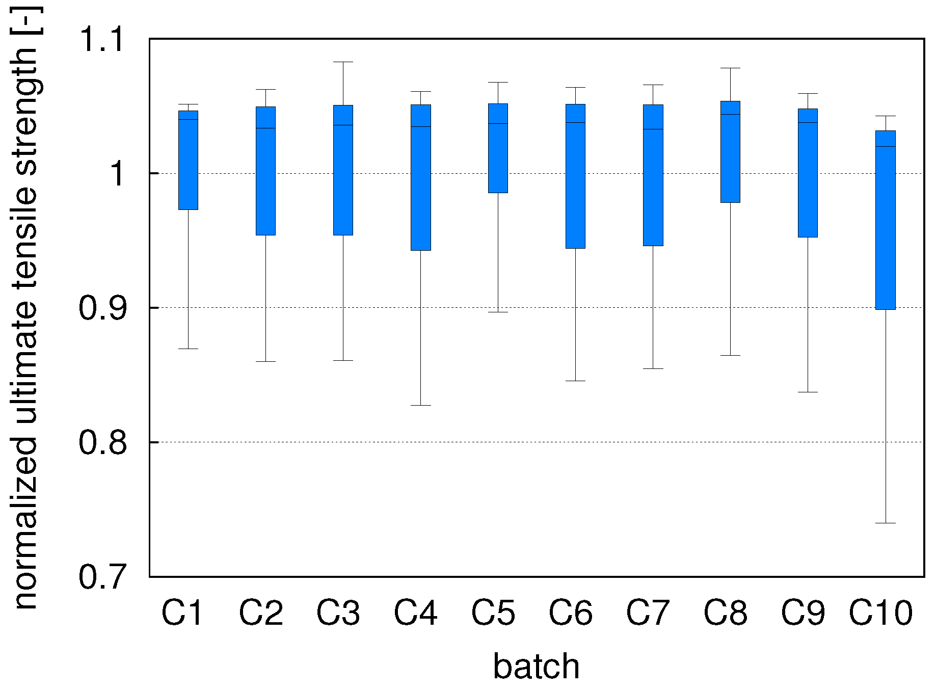
A selection of the notched samples is applied for the validation of the FLCs whereas the A50 samples are used in uniaxial tensile tests so that the material parameters can be obtained for both, the scatter determination and fitting purposes. These results are presented batch wise in terms of the normalized ultimate tensile strengths of the specimens. For the statistical analysis of the tensile test results, only the results of the A50 samples are considered.

The samples are selected in such a way that they can capture the largest scatter. The ultimate tensile strength of the material is selected as the decisive parameter since it is associated to the initiation of the necking. The stress distribution is represented in a box and whisker plot in Figure 11 for the A50 samples.

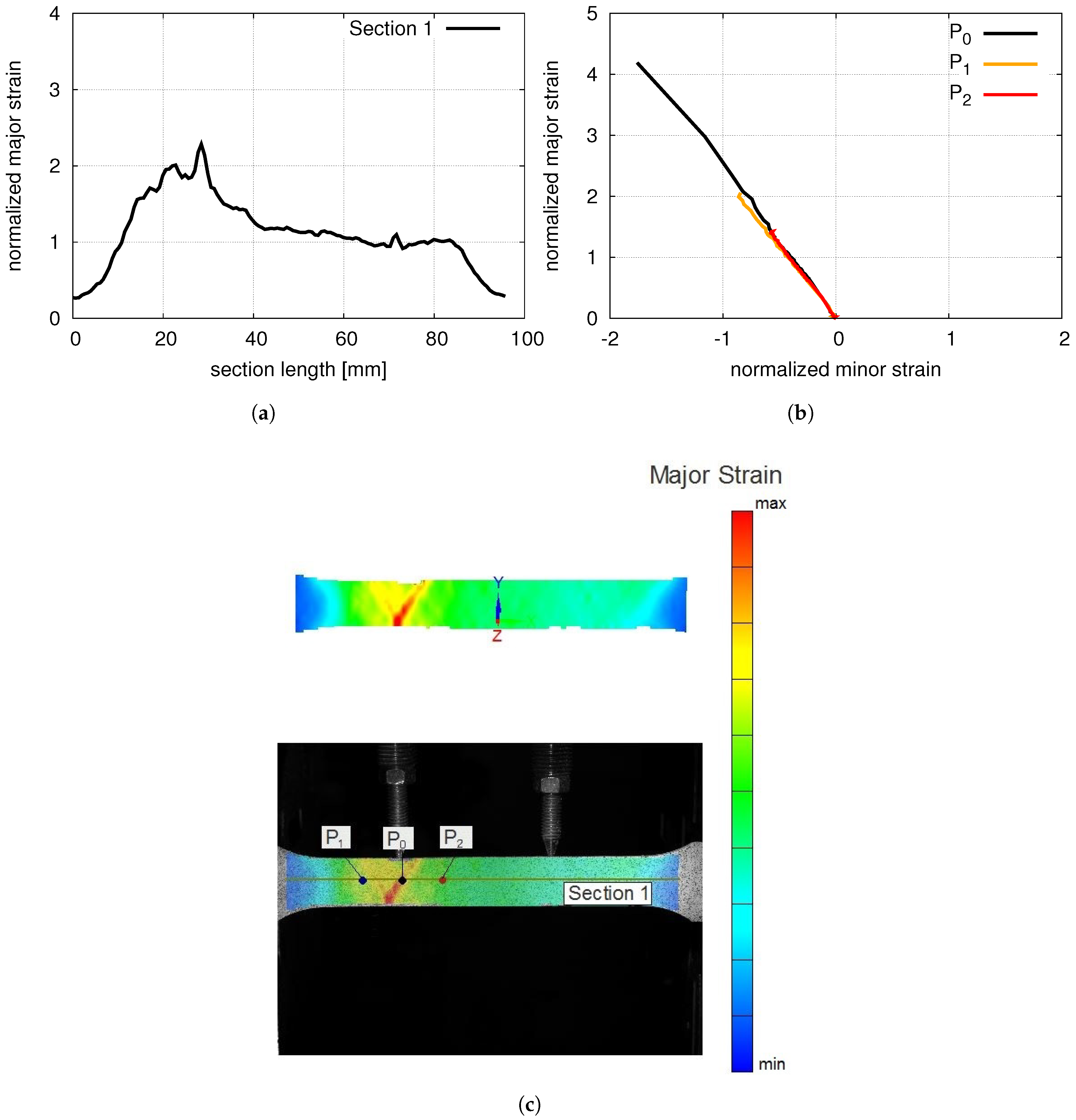
The onset of material instability can be observed from the exhibition of the shear bands as depicted in Figure 12. These bands correspond to an abrupt loss of homogeneity in deformation. Hereafter, the localized deformations rapidly intensify, leading to necking and rupture of the specimen. Figure 12a shows the non-uniform strain distribution along the section length in the pre-failure regime. The closer to the shear band, the greater the localized strain. Points 0, 1 and 2 in Figure 12b,c illustrate different major strains under uniaxial loading. Since point zero ($P_0$) lies on the shear band, it undergoes severe strains. In contrary, points one and two ($P_1$ and $P_2$) show much smaller strain values as they locate far from the shear bands where the localized necking occurs.

According to Werner [34], the ratio $\beta$ of the increment of the effective plastic strain in the non-necking region $(d{\overline{\epsilon }}_{P_i},i=1,2)$ to that of the necking region ($d{\overline{\epsilon }}_{P_0}$) indicates the plastic instability expressed as

$$\beta =\frac{d{\overline{\epsilon }}_{P_i}}{d{\overline{\epsilon }}_{P_0}},i=1,2,$$

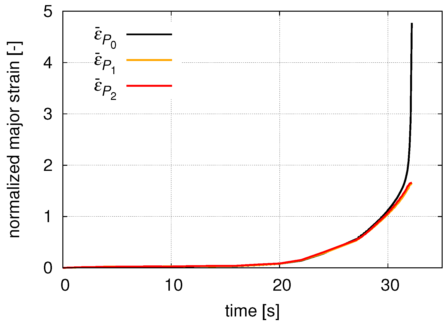
where the points $P_1$ and $P_2$ belong to the non-necking region and the point $P_0$ belongs to the necking region (refer to Figure 12). Additionally, the growth of the major strains at the aforementioned points are plotted with respect to time in Figure 13.

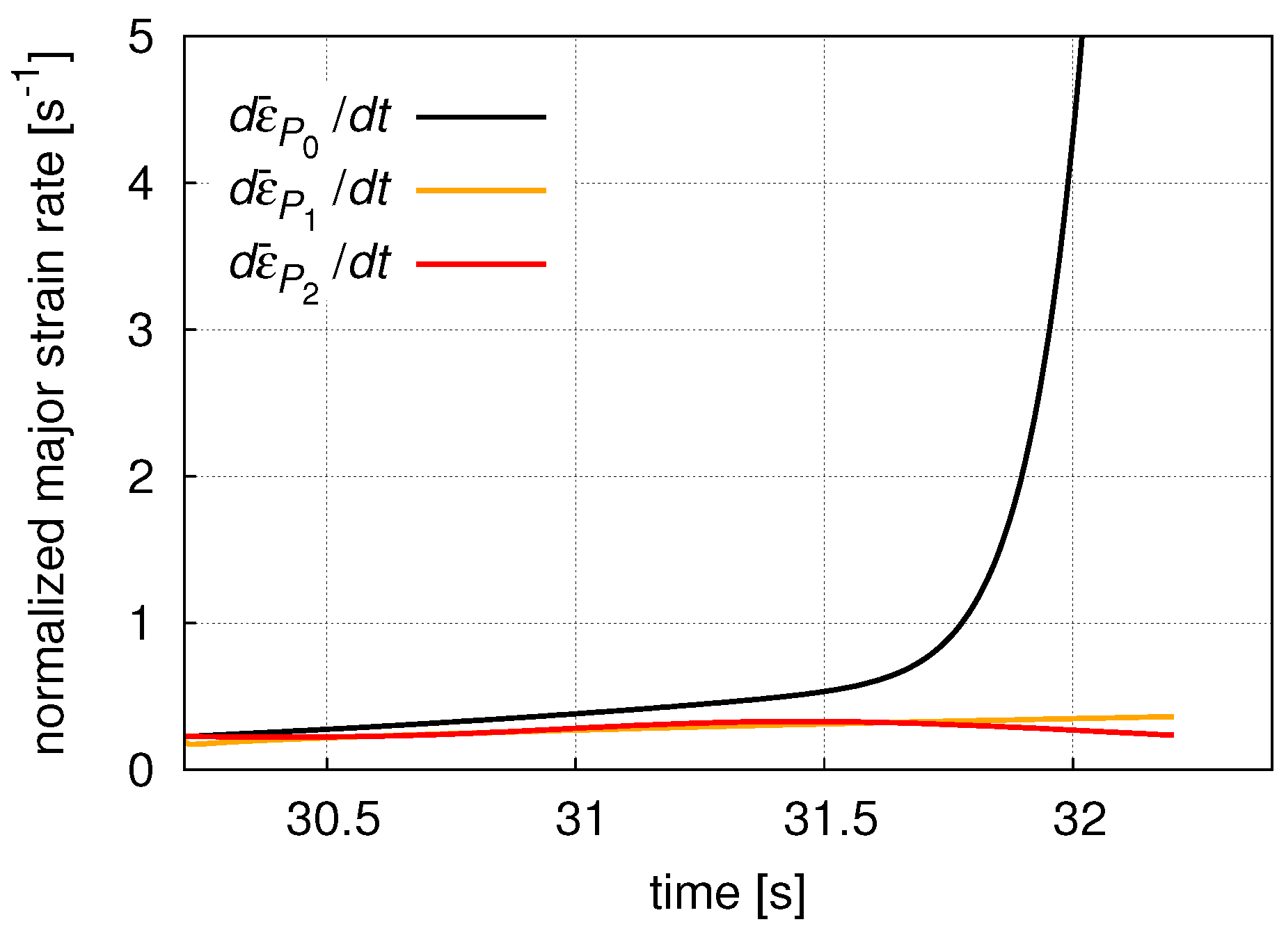
In order to guarantee the accuracy of the strains during the abrupt localization phenomenon, a frequency of 10 frames per second is applied in the tensile tests. At point $P_0$, exponential growth of strains is observed. This is not the case at other points ($P_1$ and $P_2$) far away from the necking region. However, this can be better illustrated in terms of the strain rates. Figure 14 shows the last two seconds before a sample ruptures. At this time, strain rates in the necking region ($P_0$) observe a sharp increment whereas the ones in the non-necking regions ($P_1$ and $P_2$) end up with a slight decrease. 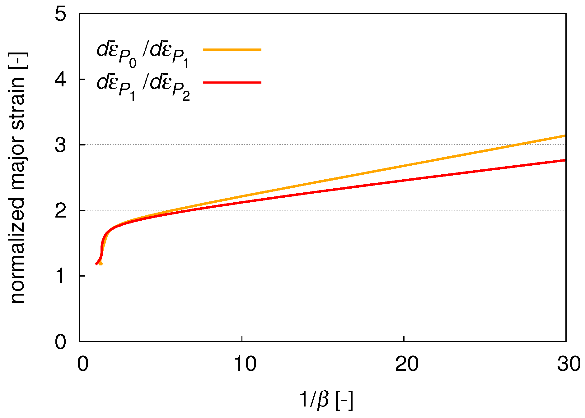This is due to the fact that from second $31.5$, all plastic strains flow though the shear band where the $P_0$ lies and the points $P_1$ and $P_2$ behave as though they are unloaded. Notice that the plastic strains remain in the latter points since they are permanent. Finally, Figure 15 illustrates the corresponding strains over the strain increment ratio ($1/\beta$). From these results, the corresponding values of the major strains for a specific ratio (here $1/\beta =10$) are extracted for each sample to prescribe the onset of the instability in the numerical solution.

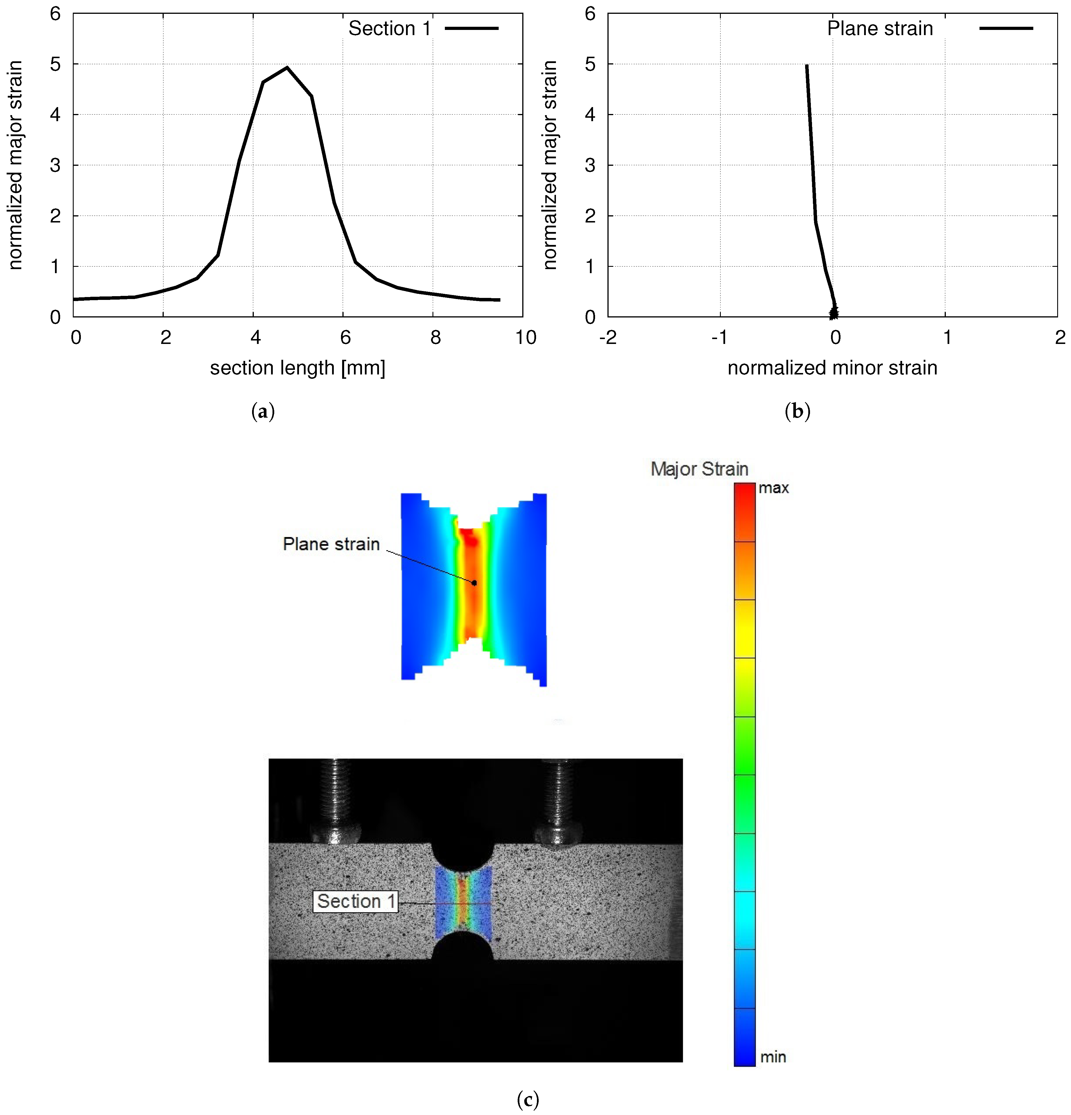
The plane strain condition occurs in the middle of the notched samples as the dimension of the sample along one direction is much larger compared to the other two dimensions. Similar to the A50 samples, the strain field is analyzed across the shear bands for determining the onset of necking. The distribution of the normalized ultimate tensile strengths of the notched samples are depicted in Figure 16. Limit strains from notched samples are used as a reference in the forming limit curves for the plane strain loading path.

Figure 17a shows the distribution of the normalized major strains along the width of the notch during necking. The stress state of a point in the middle of a notched sample of this form reflects a plane strain condition with a small deviation [36] (refer to Figure 17b). This is shown in the experimentally determined limit strain of the notched sample from ARAMIS in the necking regime (see Figure 17c) as well.

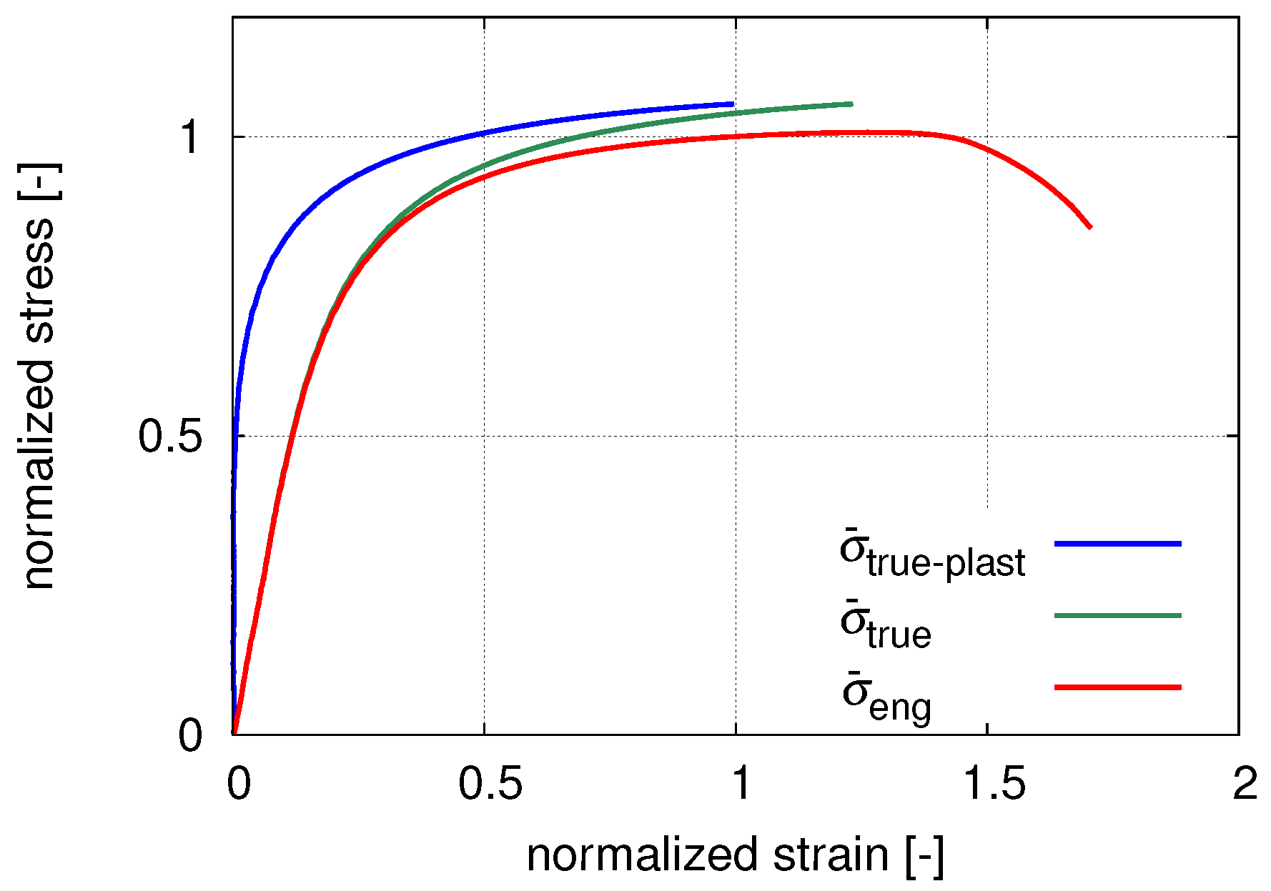
The flow diagram of the material is produced using the A50 samples to obtain the parameters related to the hardening relation (see Figure 18). As the initial cross-sectional area is considered for determining the stress values, the flow diagram typically represents the engineering stress-strain values. For sufficiently small deformations, the engineering stresses and strains are almost equivalent to the Cauchy stresses and logarithmic strains (in the sequel called “true” stresses and strains). Since the forming limit is characterized by large scale permanent plastic deformation, the hardening relations must be based on the true stress-strain values. Consequently, the engineering stress-strain diagram is first transformed to the corresponding true stress-strain diagram by the relations.

$$\begin{array}{c}\hfill \begin{array}{cc}\hfill {\sigma }_{\mathrm{true}}& ={\sigma }_{\mathrm{eng}}(1+{\epsilon }_{\mathrm{eng}}),\hfill \\ \hfill {\epsilon }_{\mathrm{true}}& =\ln (1+{\epsilon }_{\mathrm{eng}}).\hfill \end{array}\end{array}$$

(26)

This transformation is illustrated also in the stress strain curve of a sample in Figure 18.

To capture the scatter of the material, 36 different hardening curves are generated from the flow diagrams of the corresponding samples.

In Figure 18, the necking of the specimen is observed around the normalized strain of $1.4$ in the engineering flow curve (${\overline{\sigma }}_{eng}$). However, by transferring the latter into the true stress-strain curve (${\overline{\sigma }}_{true}$), only the material response until the ultimate tensile strength is considered. Due to the negligible contribution of the elastic regime (under $2\%$) in this material, only the plastic response of the material (${\overline{\sigma }}_{true-plast}$) is taken into account in fitting as well as in the numerical solution (see Figure 18) [34].

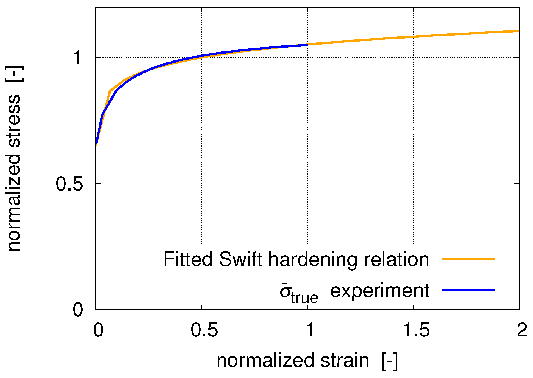
Ultimately, the curve is fitted by minimizing the square of the difference between the experimental values obtained from the plastic true stress-strain curve and the derived hardening relation from Equation (7). Figure 19 illustrates the experimental true stress-strain curve and the fitted Swift hardening relation for a specimen.

By curve fitting, the set of coefficients is generated for all 36 samples. Since equivalent stresses at regions A and B are expressed as a ratio in the residual (Equation (14)) of the mathematical model, the influence of strength coefficient $C_1$ on the limit strains is nullified. Therefore, this coefficient is kept constant in all computations. On the other hand, the variation of n results in different hardening relations and consequently different FLCs. Since the material used here is assumed to be close to rate independent, the variation of the corresponding values are not considered later in the forming limit band generation. The strain rate $\dot{\overline{\epsilon }}$ is set manually to $0.0033$ s${}^{-1}$ in the experiments (10 mm/min) whereas the strain rate exponent m is found to be $0.008$ from experiments. The evaluation of the term ${\dot{\overline{\epsilon }}}^m$ leads to the value $\dot{\overline{\epsilon }}=0.9553$, which confirms the assumption of rate-independence.

6. Forming Limit Bands

Due to the scatter in the material properties, the prediction of the failure limits by a single FLC will result in either under- or overestimation. Unlike FLCs, forming limit bands are statistical approaches towards a robust design methodology. By implementation of a band of forming limits instead of a single curve, it is possible to distinguish among safe, necking and failed zones in the forming limit diagrams.

In order to generate an FLB, first and foremost, the associated theoretical FLC model is determined. Various parameters that influence the behavior of the FLCs are identified. The material parameters are obtained from the experiments and the scatter in the mechanical properties is measured. Next, the relation between the mechanical properties and the process parameter ($f_i$) is derived. Finally, the range of the material parameters is defined by a statistical approach (here standard deviation (±2$\sigma$)) and the FLBs are generated. The generated FLBs are furthermore experimentally validated.

Different parameters obtained here can be categorized as follows:

• mechanical parameters: rolling anisotropy ($R_0$, $R_{45}$, $R_{90}$); strength coefficient $C_1$, initial yield strain (${\epsilon }_0$), hardening exponent n, strain rate exponent m,
• process parameter: measure of inhomogeneity $f_i$,
• method parameter: plastic instability indicator $\beta$.

Since the material is assumed to be planar isotropic, the influence of Lankford’s coefficients is eliminated. Moreover, as discussed in the previous chapter, the roll of the coefficient $C_1$ during the incorporation of stress ratio in the residual (Equation (14)) is omitted. Due to the assumption of rate-independence, the strain rate exponent m is applied only in the numerical calculations and therefore not varied in the forming limit curves. Since $\beta$ is defined by the user, it is not considered as a material parameter. Finally, the two parameters $f_i$ and n are needed to get the FLBs. This can be established by either fixing one parameter and varying the other or by varying both.

In spite of the fact that the inhomogeneity parameter $f_i$ has a physical interpretation, it cannot be measured in reality and thus is considered as a process parameter. Within the numerical solution, a pre-defined inhomogeneity value is set as an input for the FLC computation. This is chosen in a way to fit the FLC and is not obtained from the fitting of the hardening relations. In contrast to $f_i$, the hardening exponent n is determined through the fitting of the hardening relation to the experiments. Ultimately, both parameters define the shape of the forming limit curves.

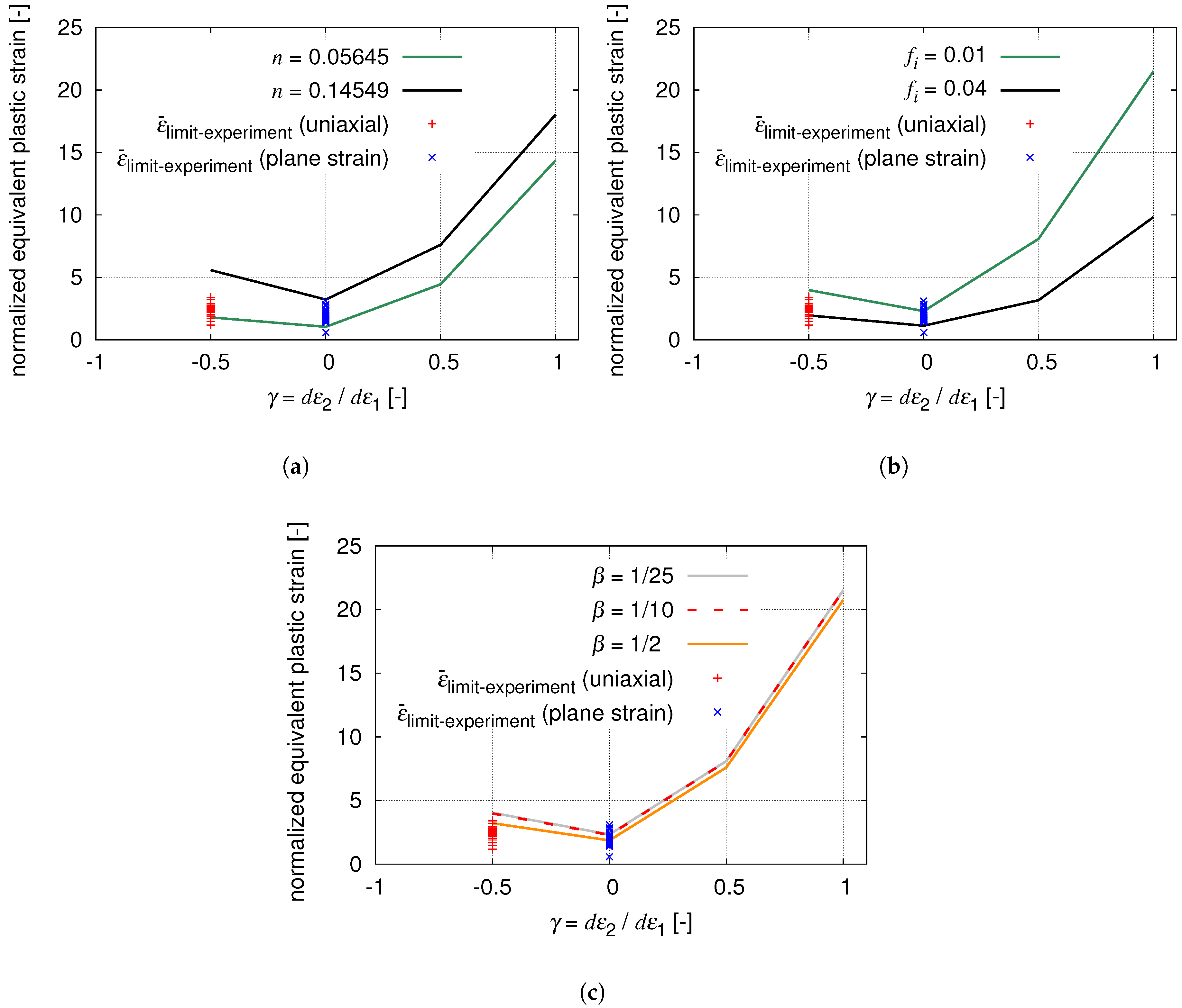
A parameter study is performed to identify the FLB and the influence of the parameters on it. The strain hardening exponent n is found to be within the range of 0.05645–0.14549 by fitting of the hardening relations to the 36 A50 samples. From Figure 20a, it is seen that the higher the value of the hardening exponent, the higher the limit strains are. In addition, experimental limit strains for uniaxial tension and plane strain states are plotted in Figure 20. The inhomogeneity parameter is kept constant ($f_i=0.02$) while altering the hardening exponent. As it is evident, for a certain value of $f_i$, two different hardening relations can contain a big range of the material scatter. However, the upper bound of the FLB corresponding to $n=0.14549$ overestimates the limit strains in the uniaxial tension regime ($\gamma =-0.5$).

Similar to the study of the strain hardening exponent, the influence of inhomogeneity parameter $f_i$ is studied in Figure 20b. In this study, the hardening exponent n is set to 0.08579 and $f_i$ is varied from $0.01$ to $0.04$ so that the FLB can capture the largest range of the the experimental limit strains for both, uniaxial and plane strain states. Lower inhomogeneity values, i.e., smaller thickness variations, result in a higher potential to resist necking. Consequently, setting $f_i$ to $0.01$ results in substantially higher limit strains than the ones with $f_i=0.04$ as shown in Figure 20b. Here, by fixing n and varying $f_i$, the FLB is not only overestimating the strains in the equibiaxial loading but also not covering the entire scatter from the experiment.

Limit strains are defined as the starting point of material instability. While generating the numerical FLC, the limiting value of the plastic instability indicator $\beta$ is considered as 0.1. However, it is not possible to denote the onset of necking by a single value. In Figure 20c, normalized limit strains with three different instability criteria are shown. It is apparent that changes in $\beta$ values do not have a strong influence on the limit strain values, provided that $\beta$ is chosen small enough. Therefore, the change of $\beta$ from $0.1$ to $0.04$ yields negligible changes in the limit strains. Nonetheless, the choice of a large value such as $\beta =0.5$ will lead to an underestimation of the limit strains.

It is observed that fixing a parameter and varying another puts a big constraint either on the numerical solution or on the form of FLB so that the material scatter is not captured anymore (see Figure 20). Therefore, both remaining parameters, namely the hardening exponent n and the inhomogeneity parameter $f_i$ must be set simultaneously.

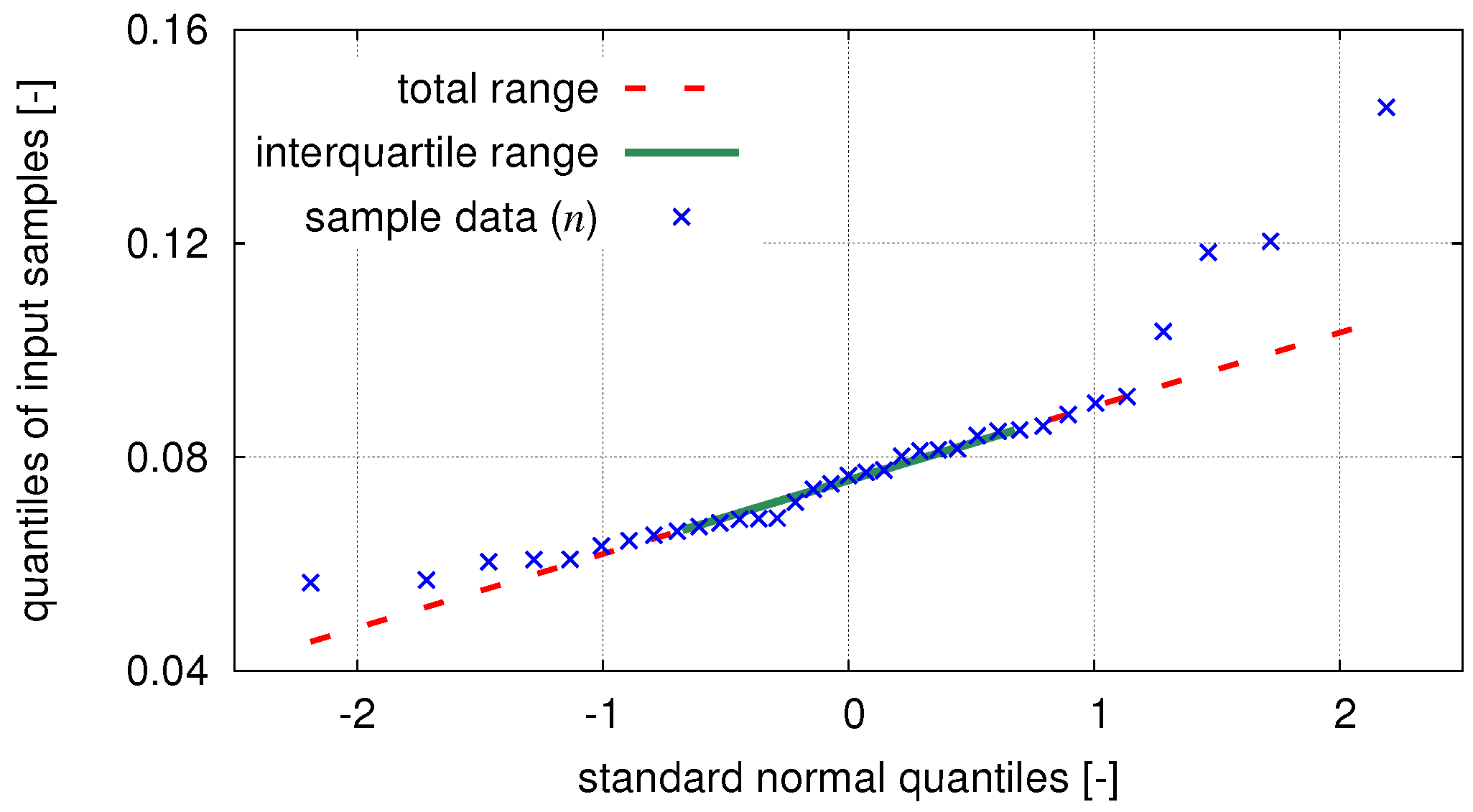
To this end, the scatter of a data set is quantified using the standard deviation. As the material scatter is expressed in terms of the hardening exponent n, the standard deviation can provide a band where most of the n values will lie. Beforehand, the normal distribution of n is checked using a quantile-quantile plot. As shown in Figure 21, results approximately follow a straight line, which indicates the distribution to be normal.

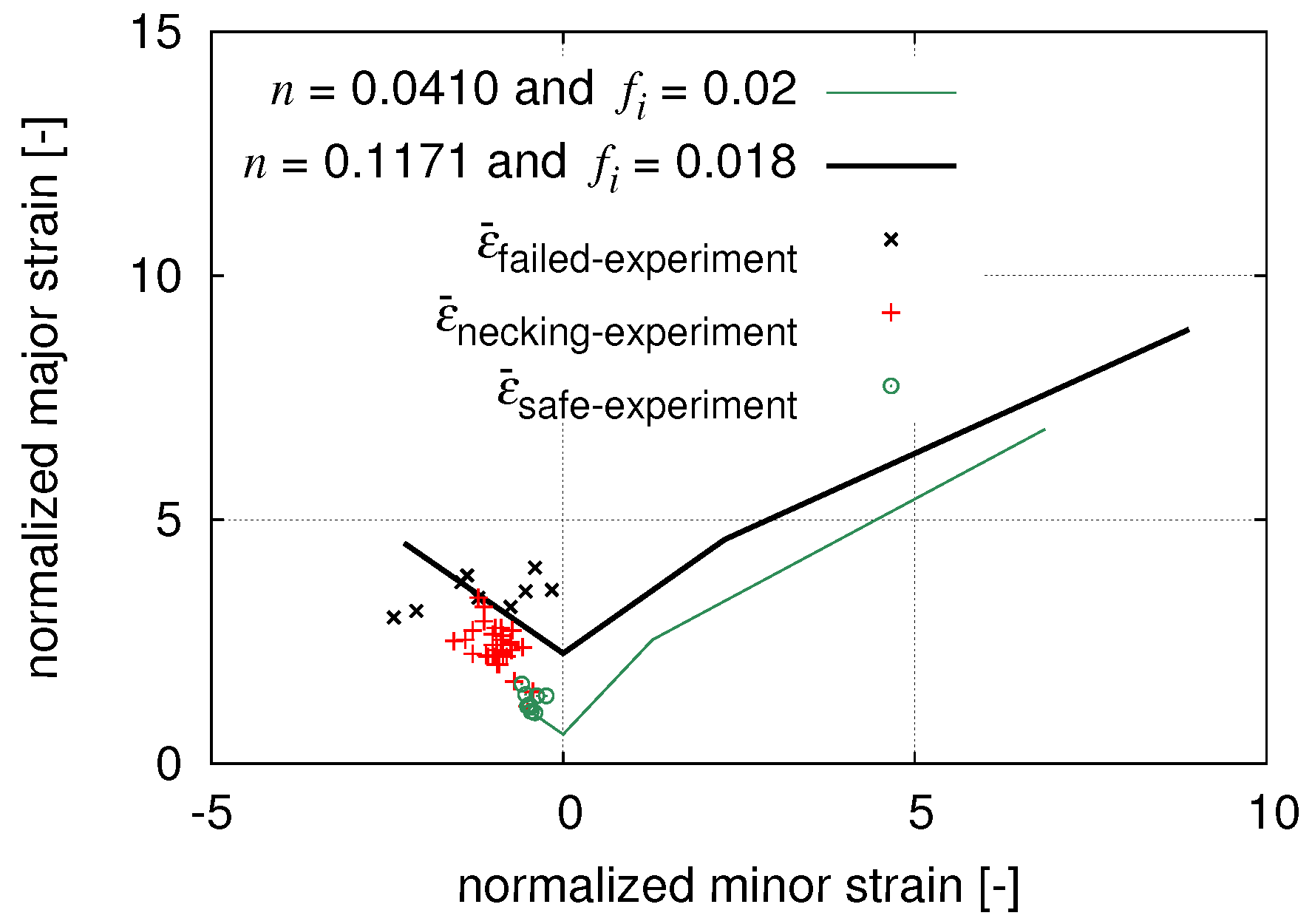
With the help of standard deviation (±2$\sigma$) of the mean ($\mu$), a band of n can be defined, which statistically contains $95.45\%$ of all values. The mean of the distribution of n is found to be $0.0791$. Employing standard deviation, the interval of n is found within the interval of [$0.0410,0.1171$]. Therefore, these limiting values of n measure the scatter in the material properties. Next, for the statistically obtained n bounds, the corresponding $f_i$ values are set to $0.02$ and $0.018$ to cover the experimentally determined limit strains.

In Figure 22, upper and lower bounds of FLB are plotted in terms of normalized major-minor strains. Experimental results of 72 representative samples are found to be within the range of numerically generated bands. Evidently, by considering a range for n and $f_i$, the FLBs divide the region into safe, necking and failed zones. Here, the failed points are captured experimentally immediately before the rupture of the specimen whereas the safe points present the strains before the onset of the necking. 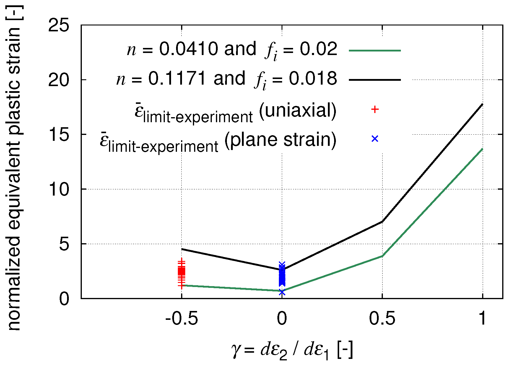Figure 23 depicts the numerically determined forming limit band in terms of equivalent plastic strains.

7. Conclusions

In the present work, a modified Marciniak–Kuczynski model with an inclined groove is implemented to generate forming limit bands. The model is derived for planar anisotropic rate dependent material. However, due to the application of manganese boron steel (22MnB5), it is simplified later to planar isotropy and rate independence. In this model, the concept of zero extension angle for the tension-compression quarter of the FLCs is applied. The form of the numerically determined FLCs is governed by different material and numerical input parameters. The material parameters are obtained by fitting the Swift hardening relation to the material response of the tensile tests. To this end, different samples are extracted from car body components and subjected to tensile loading. Since the material properties show a considerable scatter, statistical analysis is established to incorporate the scatter into the FLCs along with the numerical parameters. In order to capture the full field strains during the tests, digital image correlation is used in addition to conventional measuring systems. As expected, manganese boron-steel exhibits a considerable material scatter which cannot be captured by a single FLC. Hence, a band of FLCs, namely a forming limit band is generated by incorporating the effects of the material scatter (hardening exponent) as well as the numerical parameters, namely inhomogeneity and instability parameters. Furthermore, the material scatter is statistically analyzed to calibrate the bounds of the FLB. From the generated FLB, the limit strains of the material are segregated into various regimes, i.e., safe, necking and failure. In this way, the necking of a material during a car crash is not represented by a single curve, but by a band of curves.