Corrosion Behavior of X80 Pipe Steel under HVDC Interference in Sandy Soil


Abstract
:
1. Introduction
2. Materials and Methods
2.1. Materials
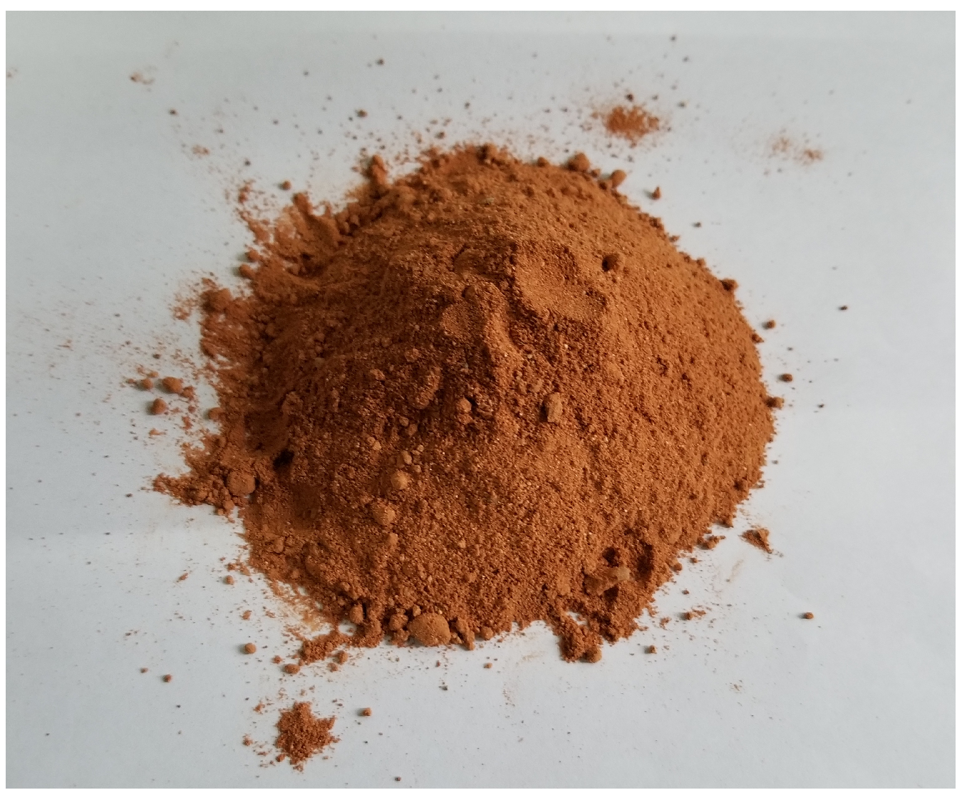
2.2. Soil Sample
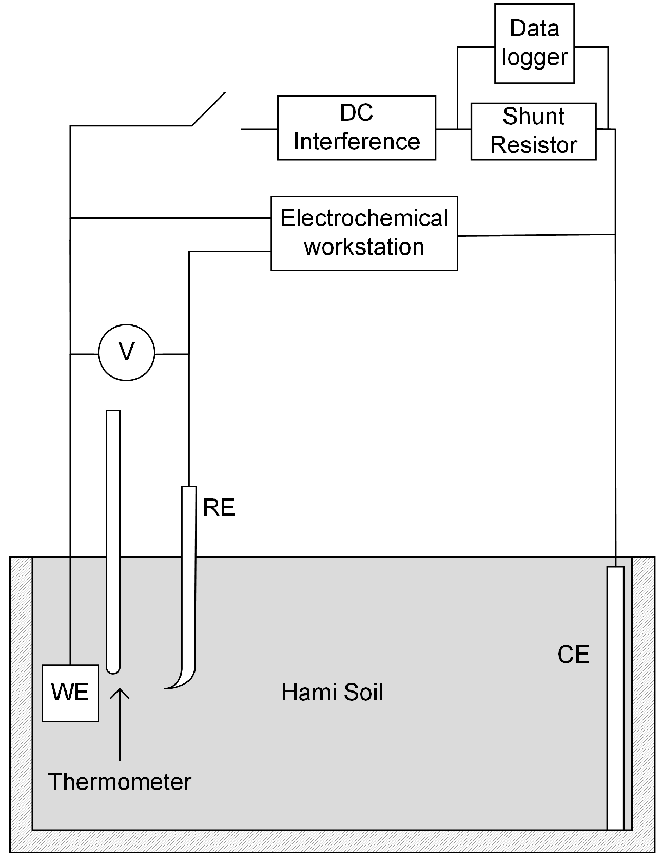
2.3. Experimental Unit
2.4. Techniques
2.4.1. Direct Current (DC) Interference Parameters Test
2.4.2. Local Soil Properties Test
2.4.3. Product Characterization
2.4.4. Corrosion Rate
3. Results
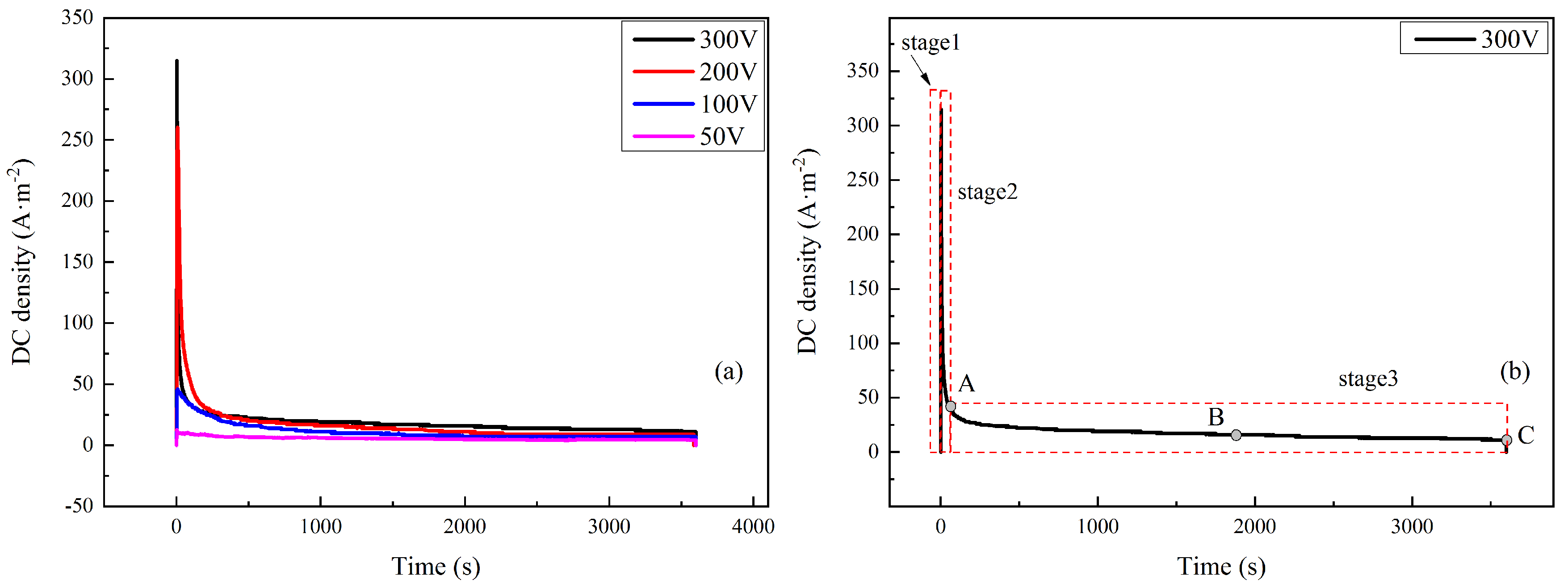
3.1. DC Interference Parameters
3.2. Corrosion Rate
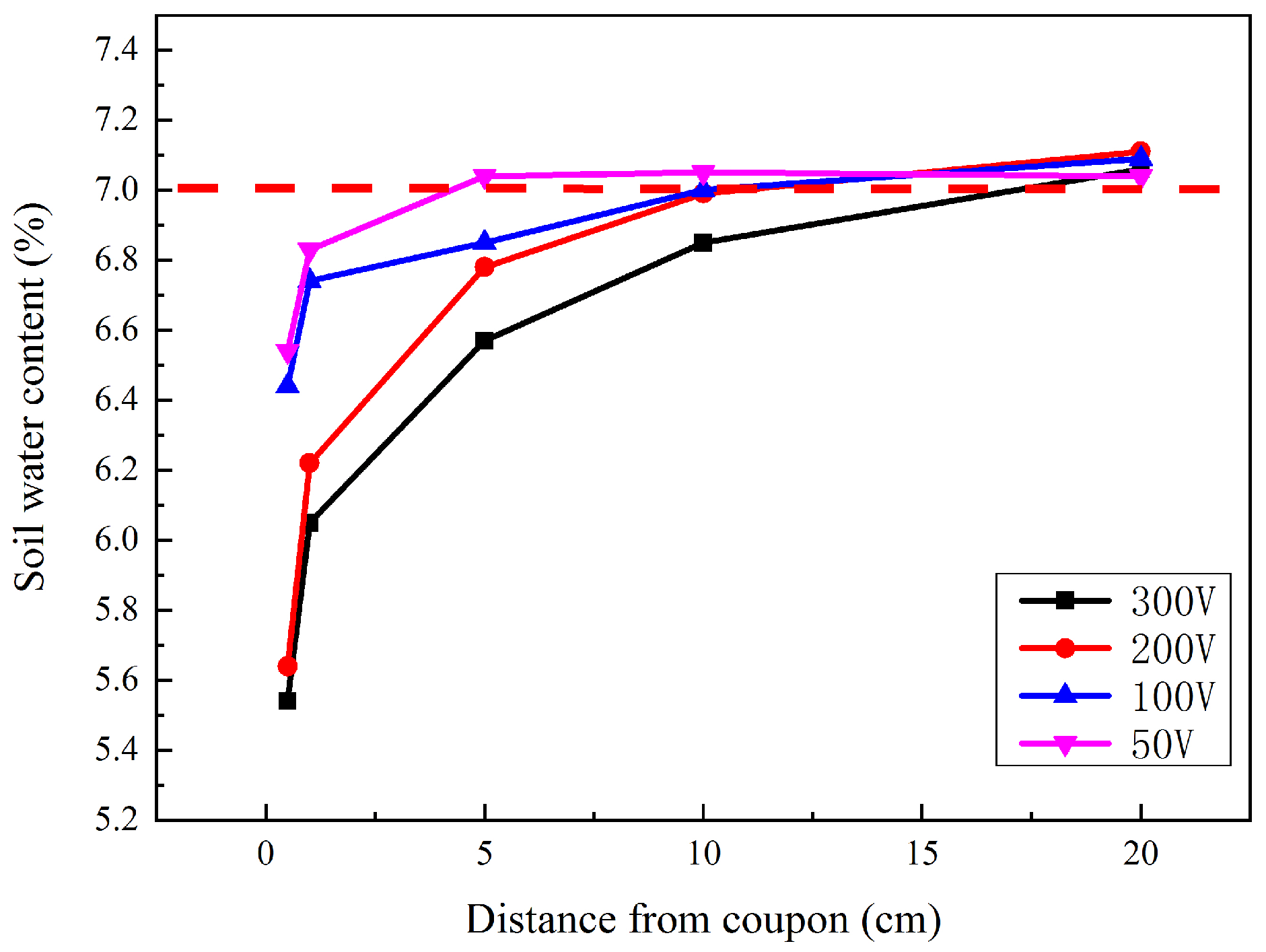
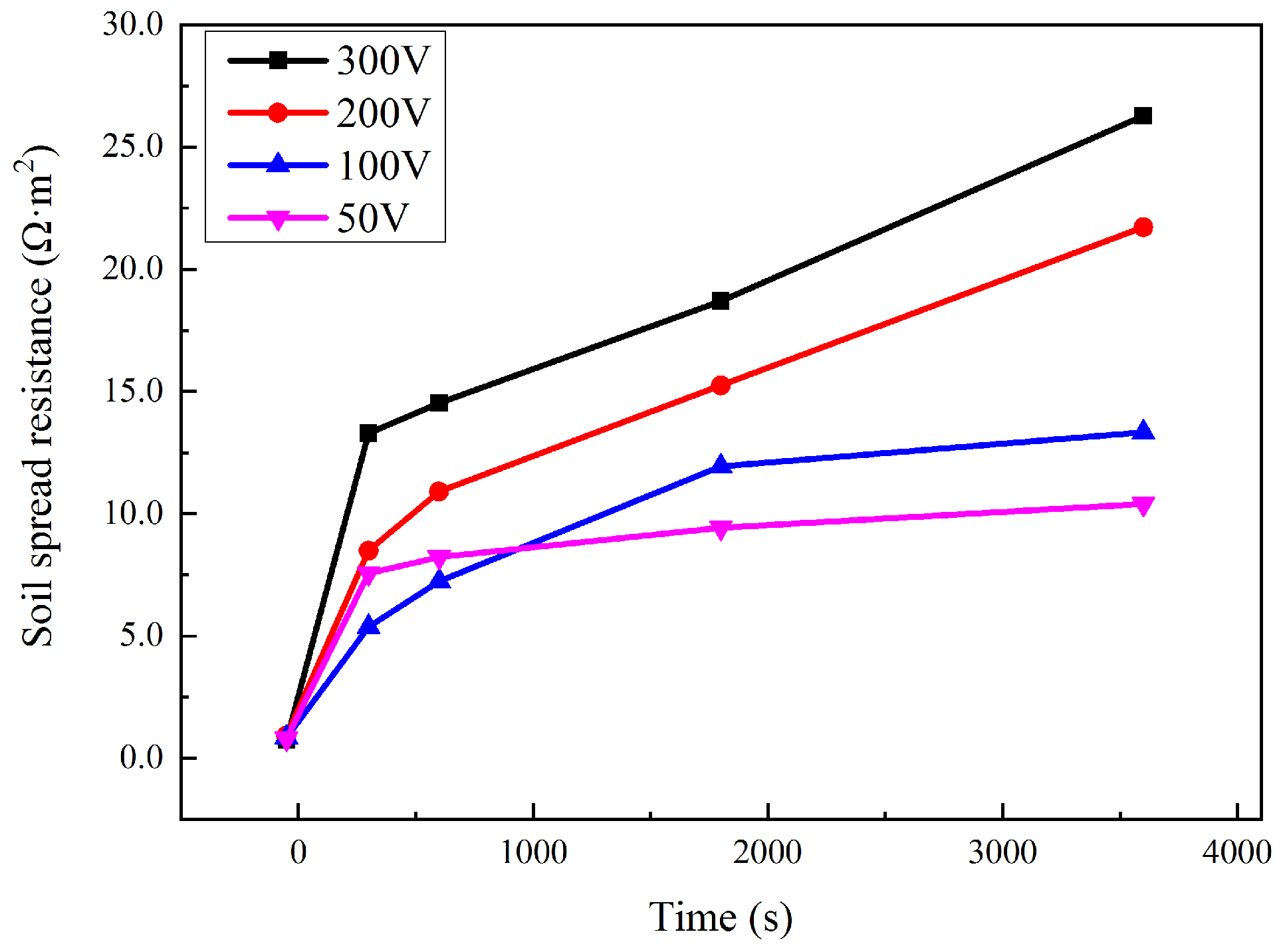
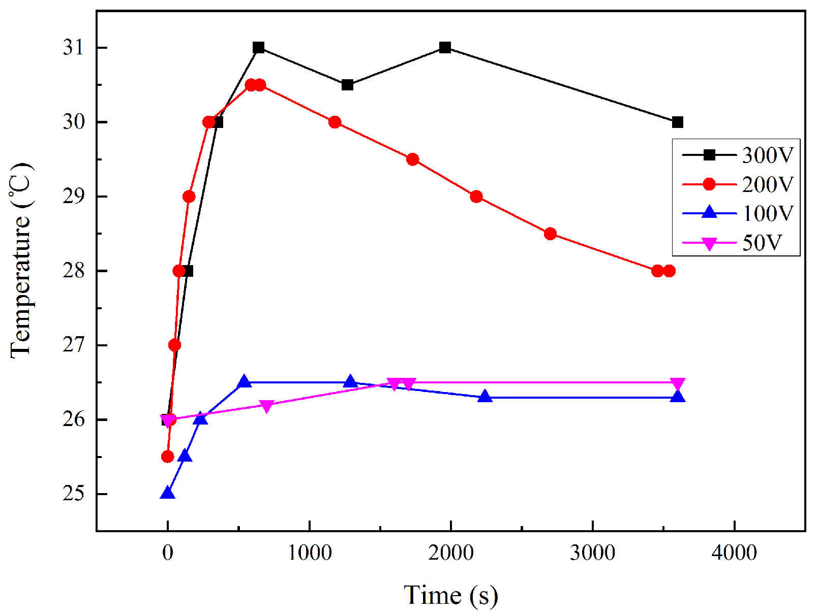
3.3. Local Soil Properties
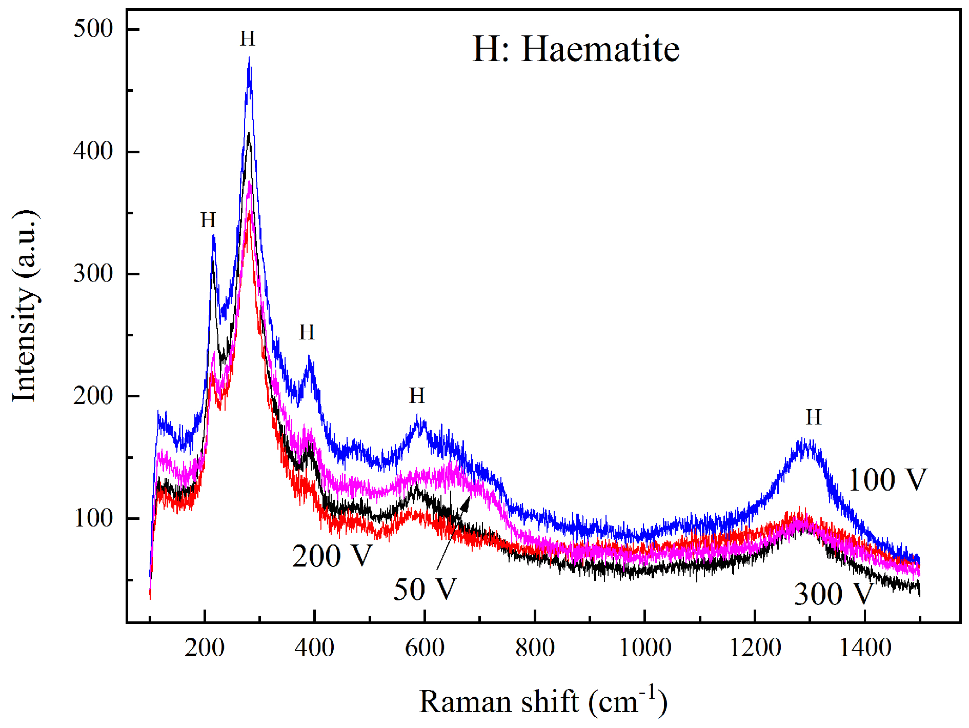
3.4. Surface Characterization
4. Discussion
4.1. Reasons for DC Density Changes under HVDC Interference
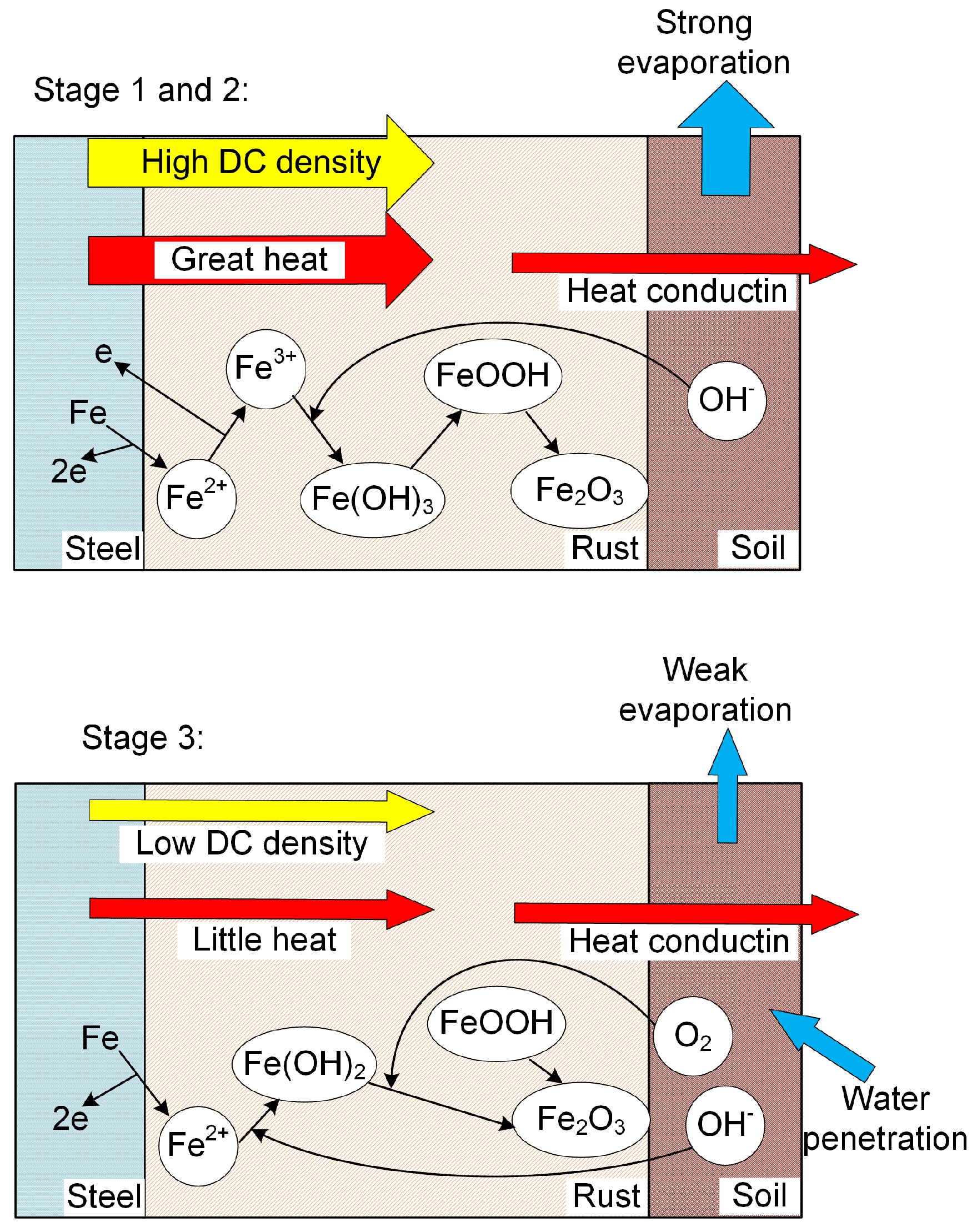
4.2. Corrosion Behavior of X80 Steel under HVDC Interference in Sandy Soil
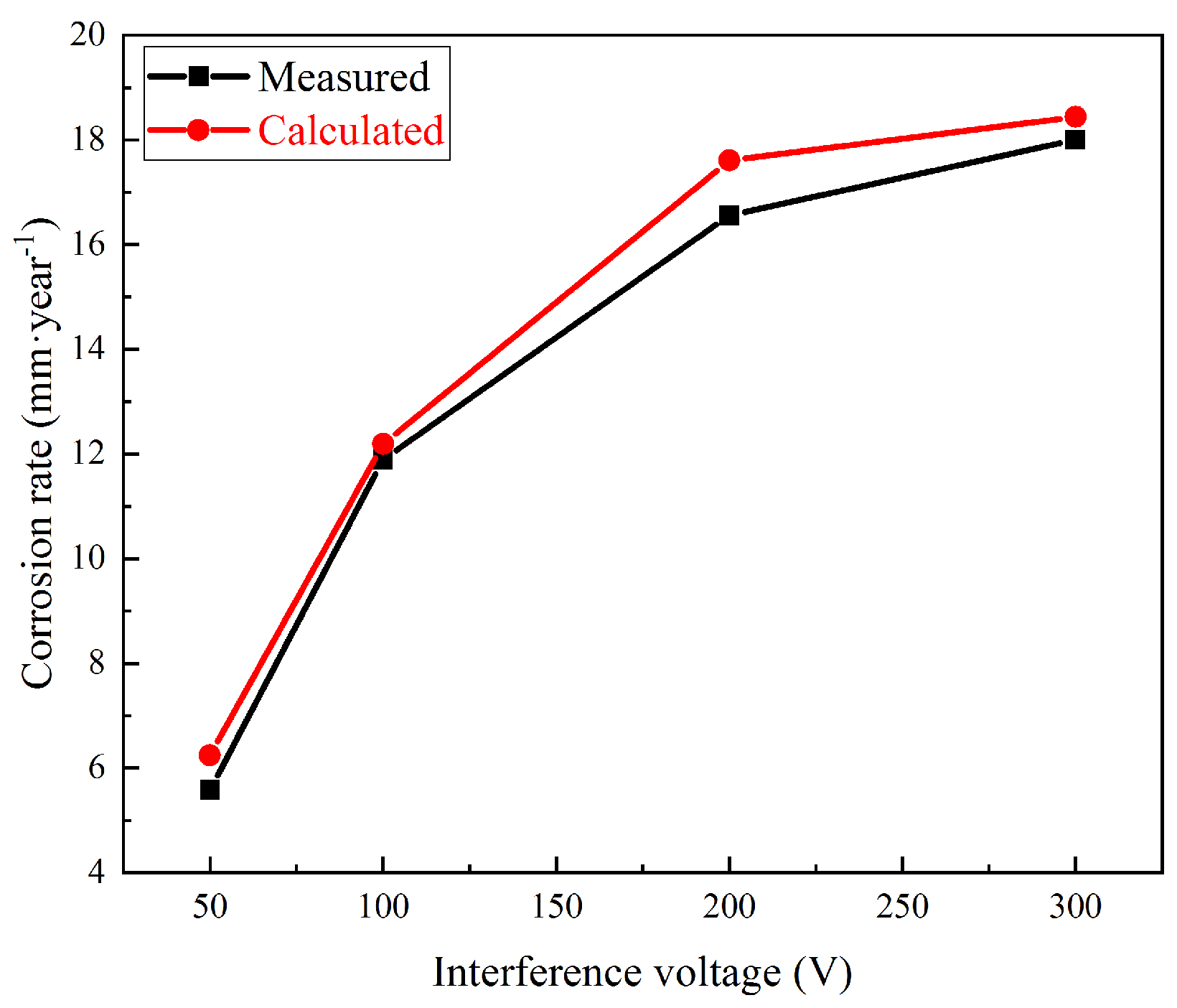
4.3. Correlation between Corrosion Rate and DC Density
5. Conclusions
Author Contributions
Funding
Acknowledgments
Conflicts of Interest
References
- Zhang, C.; Chu, X.; Zhang, B.; Ma, L.; Li, X.; Wang, X.; Wang, L.; Wu, C. A coordinated DC power support strategy for multi-Infeed HVDC systems. Energies 2018, 11, 1637. [Google Scholar] [CrossRef]
- Marzinotto, M.; Mazzanti, G.; Nervi, M. Ground/sea return with electrode systems for HVDC transmission. Int. J. Electr. Power Energy Syst. 2018, 100, 222–230. [Google Scholar] [CrossRef]
- Bahrman, M.P.; Johnson, B.K. The ABCs of HVDC transmission technologies. IEEE Power Energy Mag. 2007, 5, 32–44. [Google Scholar] [CrossRef]
- Shu, Y.; Liu, Z.; Gao, L.; Wang, S. A preliminary exploration for design of ±800 kV UHVDC project with transmission capacity of 6400 MW. Power Syst. Technol. 2006, 30, 1–8. [Google Scholar]
- Hwang, S.; Lee, J.; Jang, G. HVDC-system-interaction assessment through line-flow change-distribution factor and transient-stability analysis at planning stage. Energies 2016, 9, 1068. [Google Scholar] [CrossRef]
- Van Eeckhout, B.; Van Hertem, D.; Reza, M.; Srivastava, K.; Belmans, R. Economic comparison of VSC HVDC and HVAC as transmission system for a 300 MW offshore wind farm. Eur. Trans. Electr. Power 2010, 20, 661–671. [Google Scholar] [CrossRef]
- Verhiel, A.L. The effects of high-voltage dc power transmission systems on buried metallic pipelines. IEEE Trans. Ind. Appl. 1971, 3, 403–415. [Google Scholar] [CrossRef]
- Nicholson, E. High voltage direct current interference with underground/underwater pipelines. In Proceedings of the Corrosion Conference 2010, San Antonio, TX, USA, 14–18 March 2010. No. 10102. [Google Scholar]
- Caroli, C.E.; Santos, N.; Kovarsky, D.; Pinto, L.J. ITAIPU HVDC ground electrodes: Interference considerations and potential curve measurements during Bipole II commissioning. IEEE Trans. Power Deliv. 1990, 5, 1583–1590. [Google Scholar] [CrossRef]
- Offermann, P.F.; Schrem, F.W. The effect of HVDC ground current on oil field corrosion. IEEE Trans. Ind. Appl. 1968, 3, 260–266. [Google Scholar] [CrossRef]
- Hopper, A.T.; Gideon, D.N.; Berry, W.E. Analysis of the Effects of High-Voltage Direct-Current Transmission Systems on Buried Pipelines; Technical Toolboxes: Houston, AK, USA, 1967. [Google Scholar]
- Bi, W.; Chen, H.; Li, Z.; Jiang, Y.; Liu, L.; Hu, Y. HVDC interference to buried pipeline: Numerical modeling and continuous P/S potential monitoring. In Proceedings of the Corrosion Conference 2016, Vancouver, BC, Canada, 6–10 March 2016. No. 7714. [Google Scholar]
- Li, Z. Field test and analysis of interference of high or ultra high voltage direct current transmission system to underground steel pipeline. Corros. Prot. 2017, 38, 142–150. [Google Scholar]
- Gong, Y.; Xue, C.; Yuan, Z.; Li, Y.; Dawalibi, F.P. Advanced analysis of HVDC electrodes interference on neighboring pipelines. J. Power Energy Eng. 2015, 3, 332–341. [Google Scholar] [CrossRef]
- Qin, R.Z.; Du, Y.X.; Peng, G.Z.; Lu, M.X.; Jiang, Z.T. High Voltage Direct Current interference on buried pipelines: Case study and mitigation design. In Proceedings of the Corrosion Conference 2017, New Orleans, LA, USA, 28–31 March 2017. [Google Scholar]
- Elsener, B. Corrosion rate of steel in concrete—Measurements beyond the Tafel law. Corros. Sci. 2005, 47, 3019–3033. [Google Scholar] [CrossRef]
- McIntyre, J.D.E.; Peck, W.F. An interrupter technique for measuring the uncompensated resistance of electrode reactions under potentiostatic control. J. Electrochem. Soc. 1970, 117, 747–751. [Google Scholar] [CrossRef]
- Oelßner, W.; Berthold, F.; Guth, U. The iR drop–well-known but often underestimated in electrochemical polarization measurements and corrosion testing. Mater. Corros. 2006, 57, 455–466. [Google Scholar] [CrossRef]
- Bard, A.J.; Faulkner, L.R. Electrochemical Methods: Fundamentals and Applications; Wiley: New York, NY, USA, 2001. [Google Scholar]
- Marcus, P. Corrosion Mechanisms in Theory and Practice; Marcel Dekker: New York, NY, USA, 2002. [Google Scholar]
- Nielsen, L.V.; Nielsen, K.V.; Baumgarten, B. AC induced corrosion in pipelines: Detection, characterization and mitigation. In Proceedings of the Corrosion Conference 2004, New Orleans, LA, USA, 28–31 March 2004. No.04211. [Google Scholar]
- Nielsen, L.V.; Galsgaard, F. Sensor technology for on-line monitoring of AC induced corrosion along pipelines. In Proceedings of the Corrosion Conference 2005, Houston, AK, USA, 3–7 April 2005. No. 05375. [Google Scholar]
- Nielsen, L.V.; Nielsen, K.V. Differential ER-technology for measuring degree of accumulated corrosion as well as instant corrosion rate. In Proceedings of the Corrosion Conference 2003, San Diego, CA, USA, 3–7 March 2003. No.03443. [Google Scholar]
- Nielsen, L.V. Role of alkalization in AC induced corrosion of pipelines and consequences hereof in relation to CP requirements. In Proceedings of the Corrosion Conference 2005, Houston, AK, USA, 3–7 April 2005. No. 05188. [Google Scholar]
- Nielsen, L.V.; Cohn, P. AC-corrosion and electrical equivalent diagrams. In Proceedings of the CEOCOR 2000, Brussels, Belgium, 9–12 May 2000. [Google Scholar]
- ISO 8407:2009. Corrosion of Metals and Alloys—Removal of Corrosion Products from Corrosion Test Specimens; International Organization for Standardizatino: Geneva, Switzerland, 2009.
- Froment, F.; Tournié, A.; Colomban, P. Raman identification of natural red to yellow pigments: Ochre and iron-containing ores. J. Raman Spectrosc. 2008, 39, 560–568. [Google Scholar] [CrossRef]
- Dünnwald, J.; Otto, A. An investigation of phase transitions in rust layers using Raman spectroscopy. Corros. Sci. 1989, 29, 1167–1176. [Google Scholar] [CrossRef]
- Singh, D.D.N.; Yadav, S.; Saha, J.K. Role of climatic conditions on corrosion characteristics of structural steels. Corros. Sci. 2008, 50, 93–110. [Google Scholar] [CrossRef]
- Chitra, P.; Rajaram, R.; Venkatesh, P. Raman identification of corrosion products on automotive galvanized steel sheets. J. Raman Spectrosc. 2010, 39, 881–886. [Google Scholar]
- Nielsen, L.V.; Baumgarten, B.; Cohn, P. Investigating AC and DC stray current corrosion. In Proceedings of the CeoCor 2005, Malmoe, Sweden, 31 May–5 June 2005. [Google Scholar]
- Cao, X.; Wu, G.; Fu, L.; Jiang, W.; Zhang, X. The impact of dc current density on soil resistivity. Proc. Chin. Soc. Electr. Eng. 2008, 28, 37–42. [Google Scholar]
- Huang, Z.; Wu, G.; Jiang, W.; Xiao, H.; Guan, L. Study of the influences on soil resistivity caused by HVDC mono-polar operation. In Proceedings of the International Conference on High Voltage Engineering and Application, Chongqing, China, 9–13 November 2009; pp. 232–236. [Google Scholar]
- Sima, W.; Luo, L.; Yuan, T.; Yang, Q.; Tang, Y.; Zhou, Y. Experimental analysis on the change regulation of the soil resistivity considering the thermal effect around the grounding electrode. In Proceedings of the Asia-Pacific International Conference on Lightning, Chengdu, China, 2–4 November 2011; pp. 673–676. [Google Scholar]
- Sima, W.; Luo, L.; Yuan, T.; Yang, Q.; Lei, C.; Jiang, C. Temperature characteristic of soil resistivity and its effect on the DC grounding electrode heating. High Volt. Eng. 2012, 38, 1192–1198. [Google Scholar]
- Yan, M.; Sun, C.; Xu, J.; Dong, J.; Ke, W. Role of Fe oxides in corrosion of pipeline steel in a red clay soil. Corros. Sci. 2014, 80, 309–317. [Google Scholar] [CrossRef]
- Daub, K.; Zhang, X.; Wang, L.; Qin, Z.; Noel, J.J.; Wren, J.C. Oxide growth and conversion on carbon steel as a function of temperature over 25 and 80 °C under ambient pressure. Electrochim. Acta 2011, 56, 6661–6672. [Google Scholar] [CrossRef]
- Xu, W.; Daub, K.; Zhang, X.; Noel, J.J.; Shoesmith, D.W.; Wren, J.C. Oxide formation and conversion on carbon steel in mildly basic solutions. Electrochim. Acta 2009, 54, 5727–5738. [Google Scholar] [CrossRef]
- Cornell, R.M.; Schwertmann, U. The Iron Oxides: Structure, Properties, Reactions, Occurrences and Uses; Wiley: New York, NY, USA, 2003. [Google Scholar]
- Datta, M. Anodic dissolution of metals at high rates. IBM J. Res. Dev. 1993, 37, 207–226. [Google Scholar] [CrossRef]
- Baranwal, P.K.; Prasanna Venkatesh, R. Investigation of carbon steel anodic dissolution in ammonium chloride solutions using electrochemical impedance spectroscopy. J. Solid State Electrochem. 2017, 21, 1373–1384. [Google Scholar] [CrossRef]
- Ruby, C.; Géhin, A.; Aissa, R.; Génin, J.M.R. Mass-balance and Eh–pH diagrams of Fe II–III green rust in aqueous sulphated solution. Corros. Sci. 2006, 48, 3824–3837. [Google Scholar] [CrossRef]


| C | Mn | Si | Ni | Cu | Nb | Ti | S | P | Mo | Fe |
|---|---|---|---|---|---|---|---|---|---|---|
| 0.070 | 1.61 | 0.21 | 0.12 | 0.14 | 0.041 | 0.012 | 0.0025 | 0.0081 | 0.13 | Balance |
| SO42− | NO3− | CO32− | Cl− | Mg2+ | Na+ | K+ |
|---|---|---|---|---|---|---|
| 6490 | 101 | 3 | 3330 | 53.7 | 9300 | 200 |
| Interference Voltage (VSCE) | Peak Value of DC Density (A·m−2) | Ep after the Peak (VSCE) | Steady Value of DC Density (A·m−2) | Ep at the End (VSCE) |
|---|---|---|---|---|
| 50 | 12.8 | −0.335 | 4.4 | −0.603 |
| 100 | 45 | −0.073 | 7 | −0.523 |
| 200 | 260 | 0.992 | 9.5 | −0.429 |
| 300 | 315 | 1.052 | 11 | −0.381 |
| Interference Voltage (VSCE) | Weight Loss (mg·cm−2) | Corrosion Rate (μm·h−1) | Corrosion Rate (mm·year−1) |
|---|---|---|---|
| 50 | 0.504 | 0.638 | 5.589 |
| 100 | 1.073 | 1.358 | 11.90 |
| 200 | 1.493 | 1.890 | 16.56 |
| 300 | 1.623 | 2.055 | 18.00 |
© 2018 by the authors. Licensee MDPI, Basel, Switzerland. This article is an open access article distributed under the terms and conditions of the Creative Commons Attribution (CC BY) license (http://creativecommons.org/licenses/by/4.0/).
Share and Cite
Qin, R.; Du, Y.; Jiang, Z.; Wang, X.; Fu, A.; Lu, Y. Corrosion Behavior of X80 Pipe Steel under HVDC Interference in Sandy Soil. Metals 2018, 8, 809. https://doi.org/10.3390/met8100809
Qin R, Du Y, Jiang Z, Wang X, Fu A, Lu Y. Corrosion Behavior of X80 Pipe Steel under HVDC Interference in Sandy Soil. Metals. 2018; 8(10):809. https://doi.org/10.3390/met8100809
Chicago/Turabian StyleQin, Runzhi, Yanxia Du, Zitao Jiang, Xiuyun Wang, Anqing Fu, and Yi Lu. 2018. "Corrosion Behavior of X80 Pipe Steel under HVDC Interference in Sandy Soil" Metals 8, no. 10: 809. https://doi.org/10.3390/met8100809
APA StyleQin, R., Du, Y., Jiang, Z., Wang, X., Fu, A., & Lu, Y. (2018). Corrosion Behavior of X80 Pipe Steel under HVDC Interference in Sandy Soil. Metals, 8(10), 809. https://doi.org/10.3390/met8100809