Article

Thermal Data Optimization Through Uncertainty Reduction in Fatigue Limits Estimation: A TCM–ANN Framework for C45 Steel

by
Luca Corsaro
1,*,
Mohsen Dehghanpour Abyaneh
1,
Mohammad Sadegh Javadi
2,
Francesca Curà
1 and
Raffaella Sesana
1
1
Department of Mechanical and Aerospace Engineering (DIMEAS), Politecnico Di Torino, 10129 Torino, Italy
2
Department of Mechanical Engineering, Amirkabir University of Technology, 424, Tehran P.O. Box 15875-4413, Iran
*
Author to whom correspondence should be addressed.
Metals 2026, 16(1), 42; https://doi.org/10.3390/met16010042 (registering DOI)
Submission received: 23 November 2025 / Revised: 23 December 2025 / Accepted: 24 December 2025 / Published: 29 December 2025

Abstract

The combination of both Passive Thermography and machine learning in materials science and engineering allows rapid progress in advanced fatigue analysis. Focusing on mechanical aspects, the combination of these approaches is capable of interpolating the fatigue resistance in diverse conditions with minimal data, when compared to the classical solution, in which analyses are conducted using statistical processes such as the Staircase Method. Even though the thermal increment and thermal area are crucial parameters for the fatigue limit analysis, the implementation of machine-learning interpolation improves data consistency and reduces variability in the fatigue limit estimation through Type-A repeatability uncertainty reduction. This way, the two-layer artificial neural network does not have any predefined form of functions; second, it maintains the inherent non-linear features of the data. The validation of the proposed approach was conducted for a C45 steel, and two different experimental campaigns were conducted using a resonant machine. At the end, the analysis of the fatigue limit was conducted by means of an interpolation-assisted Two-Curve Method, starting from the classical thermal data evolution properly optimized with a machine-learning approach, achieving a more precise result in estimating the fatigue limit.

1. Introduction

The utilisation of infrared (IR) thermography began around 1930 [1]. In particular, the adoption of Passive Thermography (PT) was initiated with the objective of investigating the potential occurrence of a fire in a forest, facilitated by the advent of IR cameras. Subsequently, the potential of this technology led to its adaptation across multiple fields.
In the specific case of the mechanical field [1], the first application dates back to 1935, when PT was implemented during hot steel rolling production with the objective of measuring the process temperature. Since then, PT has become a prominent tool, particularly in applications such as production and maintenance [1]. As a matter of fact, these investigations are a typical example of the current Condition Monitoring (CM) approach [2].
In addition, IR thermography techniques were also utilised in the mechanical field for the purpose of material characterisation. The feasibility of utilising PT for temperature measurement during fatigue tests was initiated in the 1970s [3] for the purpose of fatigue crack analysis with various materials (polymer and austenitic stainless steel). Moreover, the potential of PT to detect fatigue damage was demonstrated in preliminary research applications, validating the efficacy of IR thermography. As a matter of fact, the ability of the IR detector to evaluate temperature limits during fatigue tests was introduced in [4,5], and, few years later, a new approach called the One-Curve Method (OCM) was proposed for a rapid fatigue limit estimation by the same authors [5]. In fact, a significant advantage in terms of testing time was obtained in comparison to classical fatigue testing methodologies, such as the Staircase Method [6]. On the basis of these considerations, alternative methodologies were developed for improving the fatigue limit estimation by means of PT. For instance, La Rosa et al. [7] proposed an alternative approach in which the stress amplitude values were initiated at a low level during the fatigue tests until the tested value resulted in an abrupt surface temperature increment. Another study is illustrated in [8], and an energetic approach is proposed for the fatigue limit analysis. A different approach called the Two-Curve Method (TCM) was proposed in [9]. This method estimates the fatigue limit by means of an iterative approach, and it identifies the fatigue limit by using the intersection of two linear curves. These curves approximate the surface temperature increments according to the different intrinsic dissipation mechanisms that take place below and above the fatigue limit, as also pointed out in [4]. Similar results were proposed in [10], where the authors highlighted that the fatigue limit estimation can be improved by considering the intersection of different mathematical formulations of approximating curves and thermal parameters extracted from the superficial temperature. A particular study was conducted in [11] in which an analysis of the cooling curves was also conducted. The analysis was conducted considering the gradient of the cooling curve as an alternative thermal parameter for the estimation of the fatigue limit. In conclusion, a significant number of research papers were published on the application of PT for the specific purpose of developing rapid fatigue limit estimation approaches compared to the classical methodologies, such as the Staircase Method [6]. In particular, the primary focus of the studies was on the application of mathematical formulations or the analysis of the damage evolution, with the objective of optimising the estimation process through the thermal data.
The advancement of materials science relies on knowledge about materials and how to design them for new applications. To succeed in the long term, it needs both. Due to current advancements, more and more data are now being made accessible, and huge databases give information on a variety of significant properties. When this information is linked to machine learning (ML), it opens the possibility to enhance development processes and to increase overall efficiency [12]. The use of an artificial neural network (ANN) to anticipate outcomes is deemed a potent method, as it has the capability of capturing complex and non-linear relationships, which, in many cases, can be hard to model using conventional models. This ML model creates connections between variables by identifying trends in previous observations, which is a human learning process. Such capability has rendered ANNs useful in various areas, including engineering and medicine, to finance and environmental research [13,14].
One of the major advantages of ANNs is that they are able to interpolate, or estimate data, within the range of experimental data [15]. This is especially useful in cases of highly non-linear or complex patterns [16]. This is important since the behaviour of fatigue is a highly irregular trend and relies on the interaction of variables such as stress and strain amplitude, mean stress, microstructure, surface condition, and temperature, which are not well represented by classical regression [17]. ANNs acquire these combined effects through direct learning on data and have the ability to interpolate to refine fatigue curves [18]. Park et al. [18] demonstrated that it is possible to use an Interpolating Neural Network (INN), a network architecture blending interpolation theory and tensor decomposition, to precisely fit training data without leaving interpolation theory behind, providing reliable in-range predictions. It is a clean interpolation between traditional interpolation and current deep nets to develop engineering surrogates. Bučar et al. [19] showed that neural networks (NNs) can interpolate within S–N fatigue datasets by learning underlying trends from limited experiments. It was shown that interpolating a multilayer perceptron (MLP) can be used to accurately approximate training data without abandoning the interpolation theory and allows making reliable predictions over the range.
Recent engineering has turned towards accurate and practical applications. Markovic et al. [20] tested an ANN surrogate on FE-generated data of steel parts with stress concentrators and found narrow error bands on test data. The FE geometry and load characteristics, such as notch radius and nominal stress, were used. Approximately 70% of test points fell within the range of 10% error, and approximately 87% fell within the range of 20% error. A general ML framework of fatigue life prediction across polymers and additive manufacturing (AM) alloys, proposed by Srinivasan et al. [21], demonstrated that data-efficient surrogates can be generalized with careful, reliable validation. They conducted harsh anti-leakage tests with external cross-validation of small datasets. Polymers and AM AlSi10Mg had an estimated mean R-squared of approximately 0.7, with the setup being lean. Yuan et al. [22] employed an ANN to forecast fatigue damage when the loading was non-Gaussian. It dealt well with the softening and hardening patterns and remained within the tested range. Fernández-Salas et al. [23] used Bayesian neural networks (BNNs) to predict fatigue life. Their predictions included uncertainty quantification (UQ). Their model focuses on estimating fatigue behaviour with confidence bounds rather than fitting smooth curves between data points. The work addresses uncertainty in fatigue predictions, not deterministic interpolation of limited experimental data. Table 1 shows a general overview of the existing literature and gaps that have been covered in this work.
The present research utilizes the ML method to interpolate thermal fatigue data collected in C45 steel experiments, which would allow improving the TCM method to interpolate fatigue limits. By learning nonlinear trends between thermal parameters, such as thermal increment and thermal area, the ANN is implemented in order to interpolate intermediate data points for the fatigue curve. A type of cross-validation and uncertainty reduction was also used to show the reliability of this technique for estimating the fatigue limit. Then, the uncertainty-reduction analysis quantifies and reduces scatter, increasing confidence in the estimated fatigue limit.

2. Materials and Methods

2.1. Thermographic Method

The Thermographic Method is illustrated in Figure 1. More specifically, Figure 1a presents a typical temperature profile recorded by an IR camera during a fatigue test. In general, the thermal evolution shows an initial heating phase followed by a stabilized trend. However, when the applied load exceeds the fatigue limit of the material under study, a temperature increment is observed during the fatigue test with a further abrupt rise before failure (solid red line). By contrast, if the load remains below the fatigue limit, the thermal profile stays stable (dashed red line). In order to estimate the fatigue limit based on thermal emissions generated during the fatigue tests, specific thermal parameters can be extracted from the temperature profile under each loading condition. These include the temperature increment (thermal increment, ΔT) and the area under the temperature profile (thermal area, A). The thermal parameters are calculated at a given time or number of cycles (N*), obtaining ΔT* or A*. Figure 1b outlines the procedure for the fatigue limit estimation by means of the TCM [9]. A series of tests is conducted at varying load levels, starting from an initial low value. Each load is applied until a predefined number of cycles is reached, and all tests are monitored via an IR camera. After each test, the specimen is cooled back to ambient temperature to ensure consistent starting conditions and accurate detection of the thermal evolution during the next test. The process continues until a rapid increase in thermal parameters is observed at certain load levels (indicated by blue circles in Figure 1b). The micromechanics and physical effects associated with these thermal trends have been thoroughly documented over time, as evidenced by the literature [4,5,7,8,9,10]. More in detail, at low loads, the thermal parameters exhibit a flat trend, and, subsequently, a distinct change in their evolution can be observed. These two different behaviours reflect the nature of the intrinsic dissipation involved inside the material when it is subjected to cycling loading. More in detail, below the fatigue limit, the intrinsic dissipations are primarily due to anelastic phenomena or internal damping, while microplastic deformation and dislocation movements dominate above the fatigue limit. This transition zone enables the estimation of the fatigue limit.
Over the years, various combinations of approximating curves have been proposed in the literature to model the intrinsic dissipation evolution. These include purely linear curves as well as mixed formulations involving linear, parabolic, and power-law mathematical formulations. Such diversity in curve selection reflects the complex evolution of intrinsic dissipations that occur during the fatigue damage process. When different curve types yield varying estimates of the fatigue limit, the result is typically determined using the most conservative value obtained from the application of different approximating curves and thermal parameters.

2.2. Experimental Procedure

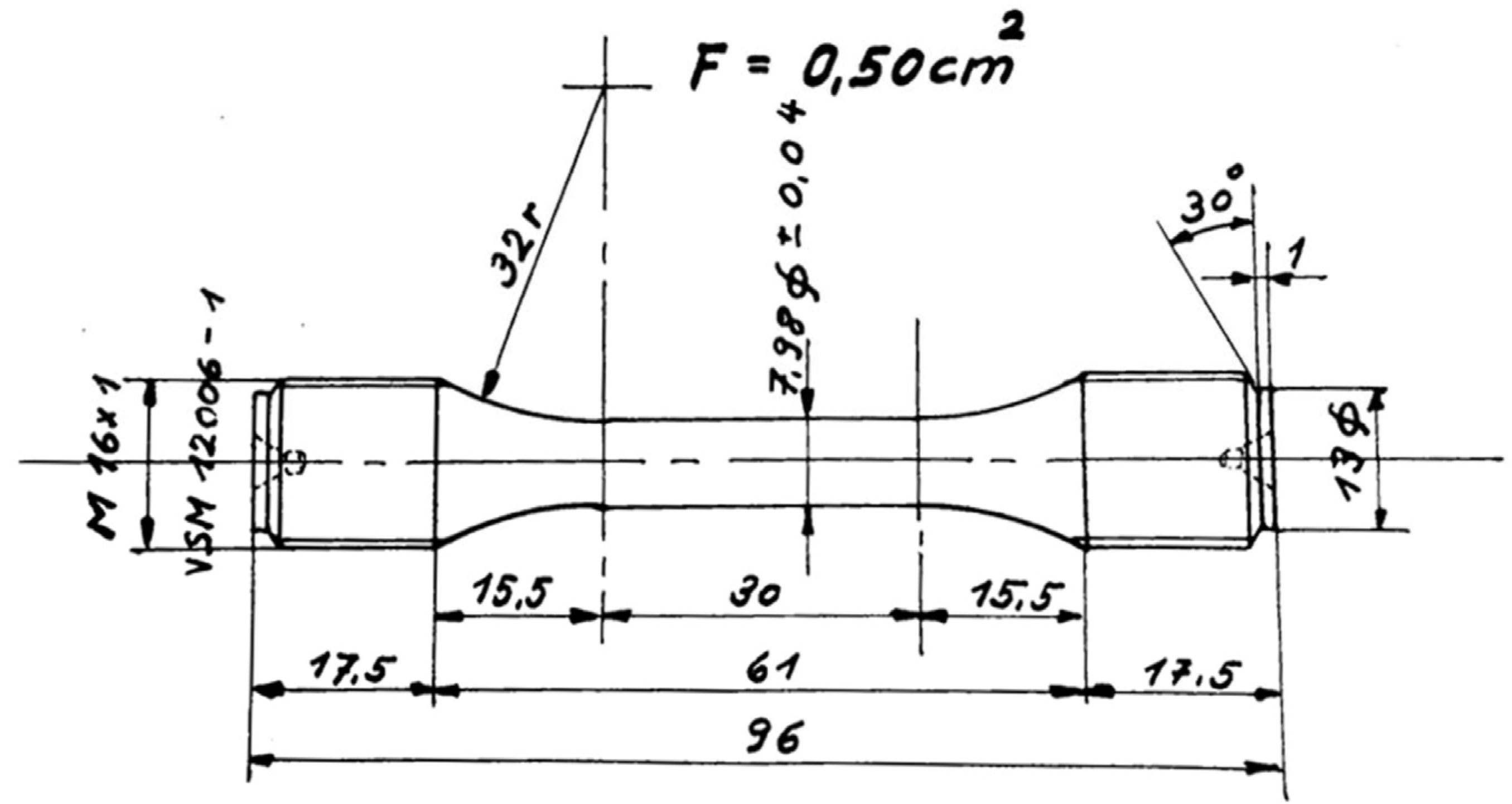
The TCM optimization by means of ML approaches was carried out considering previous experimental fatigue data reported in [24]. In more detail, the data obtained from C45 steel samples were considered. More in detail, cylindrical samples were utilized during the experimental fatigue tests, and the technical drawing according to resonant machine requirements is illustrated in Figure 2.
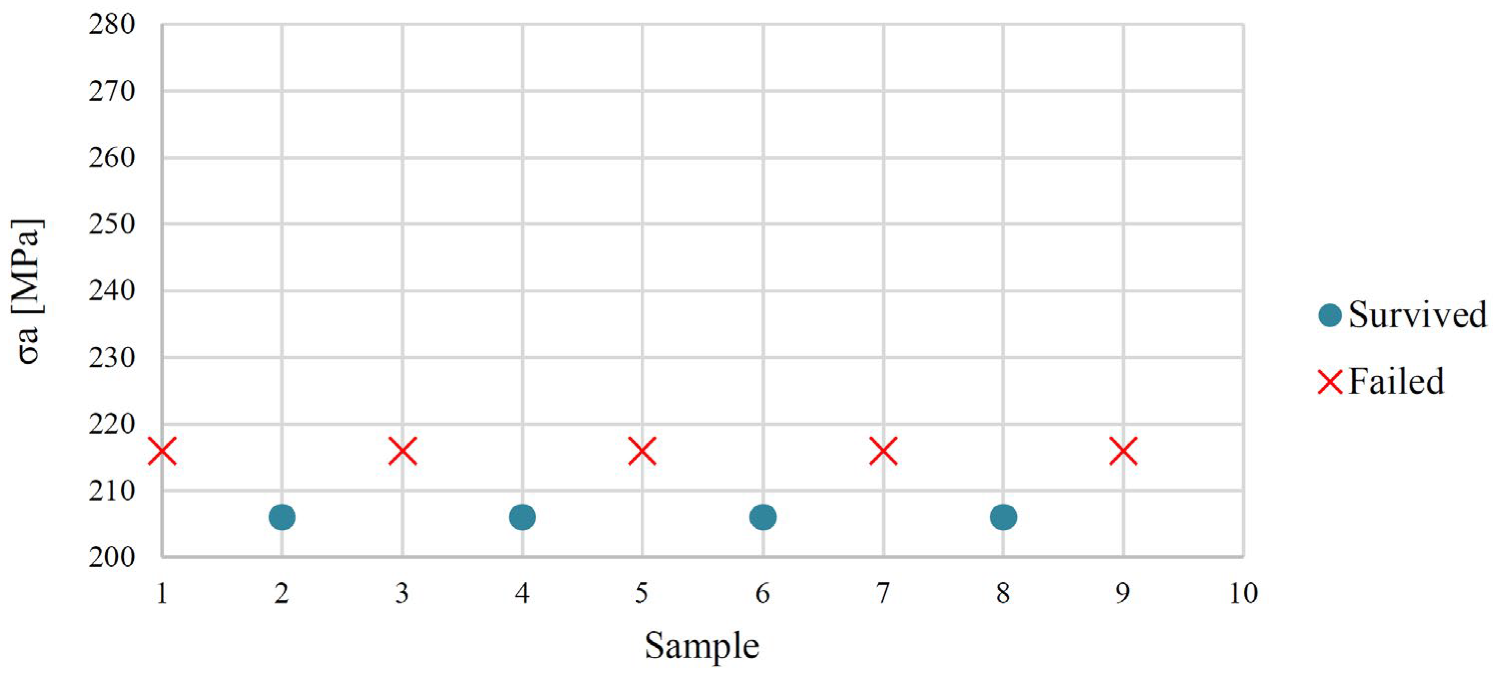
The fatigue limit was evaluated following both the Staircase Method [6] and the PT approach, specifically the TCM, with the aim of comparing the obtained results. This way, the Staircase Method provides a robust benchmark for validating the overall results since it refers to a standardized procedure. On the other hand, two distinct experimental campaigns were conducted utilising the PT approach with the objective of generating multiple fatigue limit results considering the TCM with varying thermal parameters and approximating curves [9,10]. The experimental fatigue tests were conducted with a resonant machine, operating at a testing frequency of 136 Hz. In order to facilitate a detailed comprehension of the experimental campaign to which this work refers, Figure 3 presents the results obtained from the fatigue tests, as outlined in [23]. More in detail, the classical runout (symbolised by blue dot symbols) and failure (symbolised by red cross symbols) trend, on the basis of the adopted load, is reported as a function of the sample under testing. The number of cycles for the runout condition was set equal to 2 million, and a total number of 9 samples was adopted for the fatigue limit evaluation according to [6]. During the utilisation of the Staircase Method, the load ratio was approximately 0.
Table 2 presents the results obtained from the overall fatigue experimental campaign. More in detail, the fatigue limit results obtained by means of the Staircase Method are referred to 50% ( σ D , 50 % ) and 1% ( σ D , 1 % ) probability of failure (see first column of Table 2—Staircase Method, 50% probability and 1% probability). Subsequently, the results obtained by utilising the PT approach are presented, and the fatigue limit was estimated by adopting the TCM, taking into account various approximating curve typologies and thermal parameters. In particular, the parabola–power law and the linear–linear approximating curves were adopted during the fatigue limit computation (see second column of Table 2—PT approach (TCM), approximating curves). The fatigue limit estimation was conducted by considering the analysis of two different thermal parameters detected during the fatigue tests (see second column of Table 2—PT approach (TCM), thermal parameters), the thermal increment (ΔT), and the thermal area (A), respectively. Then, the results of the fatigue limit estimation were presented on the basis of the first (σDTCM-1) and second (σDTCM-2) experimental campaign conducted during the fatigue tests (see last two columns of Table 2—PT approach (TCM), first experimental campaign and second experimental campaign). The estimation process for the two experimental campaigns was conducted in a way that was consistent with the approach outlined in Section 2.1. More in detail, subsequent to the recording of thermal profiles for each load, the thermal parameters (thermal increment and thermal area) were reported as a function of the stress amplitude that was adopted during the fatigue tests. After that, the fatigue resistance was calculated by approximating the thermal parameters evolution through the use of various mathematical formulations (for example, parabola–power law or linear–linear). These formulations were used to approximate the thermal parameters evolution for both the possibilities of thermal parameters considered in the activity (thermal increments or thermal area).
The results obtained with the PT approach were achieved with a significant advantage in terms of testing time compared to those evaluated with the Staircase Method. However, variability was observed in the estimation of the fatigue limit when different thermal parameters were utilised, and various approximation curves were used during the calculation. This is necessary because the fatigue limit is unknown in the case of application of the Thermographic Method for the fatigue limit estimation, and different combinations of thermal parameters and approximating curves are generally adopted during the analysis to detect variability in the estimated results.

2.3. Artificial Neural Network (ANN)

The artificial neural network (ANN) is a data-driven method of predicting fatigue response without a particular constitutive or life model [25]. Another application of this ML method can be related to the interpolation between the stress amplitude [26]. In fatigue tests, mechanical energy is partially lost as heat, and temperature response provides first-hand information on the progression of damage. Two key thermal indicators are derived from the PT data in order to measure this behaviour. The two parameters are both dependent on the amplitude of stress applied and hence are closely associated with fatigue strength. When the fatigue strength is plotted on the horizontal axis and the thermal parameters (ΔT and A) are plotted on the vertical axis, the curves that are obtained show the development of the thermal behaviour of the material as the loading intensity nears the fatigue limit. Interpolation by the ANN technique allows for adjusting the weights of its connections as it learns from experimental data [15]. The curve with interpolated points was then used for the TCM to find results. This process paves the calculation of the fatigue limit with increased accuracy. According to a previous study [26], ANN and GPR provided acceptable results for interpolation. However, SVR performed less favourably. Choosing the ANN is not related to the universal superiority of this method. Therefore, in this study, the ANN is used as a within-domain interpolation tool. The objective of the ANN is not generalization or prediction outside the experimental domain. This technique is used as an interpolation-assisted TCM workflow.
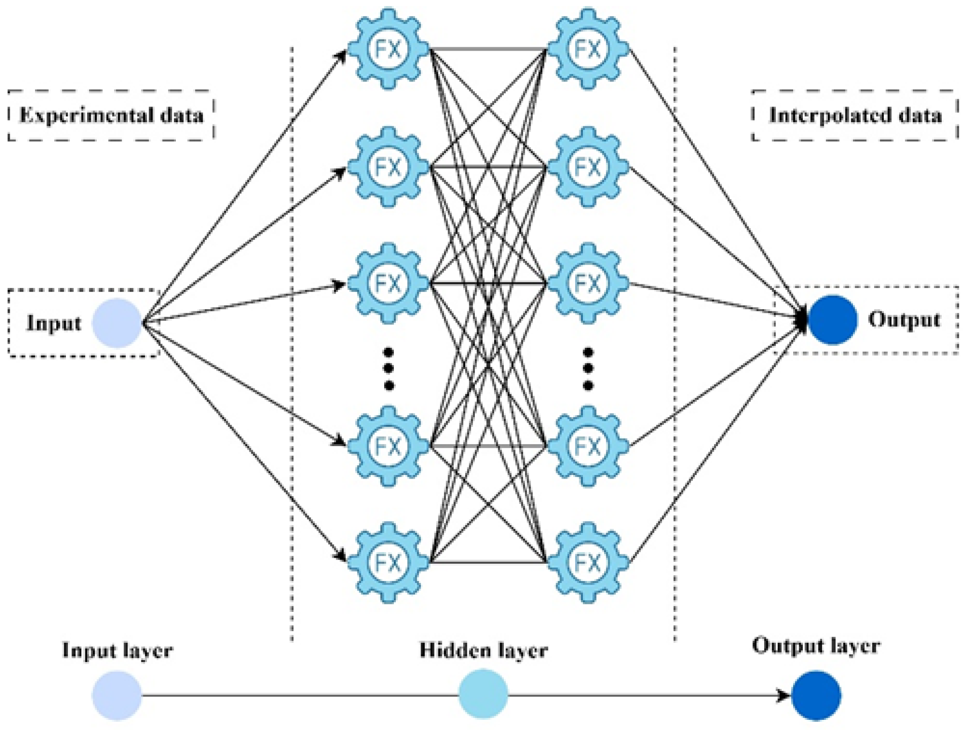
ANNs consist of several layers of connected neurons, and the number of layers is an important factor in the ability to solve problems [27]. Single-hidden-layer networks are usually adequate to perform usual tasks [28]. Deep neural networks (DL) having several hidden layers are formulated to handle more complicated tasks, such as pattern recognition, image analysis, and natural language processing [29]. Python 3.10 was trained and selected on early stopping in Colab to reach the best method. In the code, two important hyperparameters, the network size (hidden-layer configuration) and the L2 regularization strength (alpha), were tuned. For this, a small grid search was performed with early stopping applied during training. Some hyperparameters were fixed to reduce degrees of freedom. Table 3 shows some fixed hyperparameters and the two optimised ones with their range. According to the authors of [26], a method of interpolation was designed, and a target of R 2 0.99 was fixed in this work. In this study, a two-hidden-layer network was chosen as the best to interpolate data more precisely. The architecture of the ANN used for interpolation in this study is shown in Figure 4. Therefore, the ANN is used as an interpolation tool that is flexible without presuming to be superior to other techniques; it is integrated into the TCM workflow.

2.4. Accuracy Metrics

Mean Squared Error ( M S E ) or Mean Squared Deviation (Equation (1)) is used to measure the squared differences between the actual and the interpolated values. A smaller M S E , which is near zero, means that the interpolation closely matches the targeted data. Root Mean Squared Error ( R M S E ), also known as Root Mean Squared Deviation (Equation (2)), is the square root of the M S E . This is the standard deviation of the interpolation errors, which expresses how well the fitted curve fits the data points. Mean Absolute Error ( M A E ) is an expression of the mean absolute difference between the interpolated and observed values. As compared to M S E , which puts greater emphasis on larger deviations, M A E is a simple measure of average error in the same units (Equation (3)). Mean Absolute Percentage Error (MAPE) compares the interpolation accuracy on a relative basis. It also expresses the errors as percentages of the actual values. Although it is helpful when relative changes are of more importance than absolute values, MAPE also has disadvantages, including that it is sensitive to unreliable or near-zero values. This can lead to distorted or misleading errors. Therefore, this metric is not considered a primary performance metric due to the fact that its application can be curtailed in situations where interpolation can result in large deviations [30]. In the case of ANNs and other ML techniques like GPR or SVR, the Coefficient of Determination ( R 2 ) is more difficult to interpret when used with non-linear regression models or interpolation. In contrast to simple linear regression, R 2 is not necessarily limited to the range 0 to 100 percent and, in some circumstances, may even be negative (Equation (4)). A negative R 2 value implies a poor interpolation performance, and the model does not capture the underlying structure of the data and giving inaccurate results. However, high R 2 values in small datasets show goodness of fit rather than robustness. This effect is particularly relevant for flexible models, which may generate smooth interpolants. This is why it is not always sufficient to use R 2 as the sole indicator of the quality of interpolation. Supplementary error measures like M S E , M A E , and R M S E are more reliable, especially when the data do not follow a simple trend or an easily observable trend [31].
M S E = 1 n 1 n Y p r e Y a c t 2
R M S E = 1 n 1 n Y p r e Y a c t 2
M A E = 1 n 1 n Y p r e Y a c t
R 2 = 1 1 n Y p r e Y ¯ p r e 2 1 n Y a c t Y ¯ a c t 2
In the above equations, Y a c t is the actual output value of the dataset, Y p r e is the predicted output value of any machine learning algorithm, Y ¯ a c t is the mean of the actual output, and Y ¯ p r e is the mean of the predicted output [16,28,32].

2.5. Cross-Validation Strategy

In this study, the predictive ability of the model for interpolation was evaluated. With the Python Colab M17.1 implementation, the Leave-One-Out Cross-Validation (LOOCV) approach was used. Since only ten experimental data points were available, in each iteration, one point was left out as the test sample while the model was trained on the remaining nine points. At each fold, the ANN is re-initialised and re-trained from scratch using only the training subset. For each run, the normalization procedure was performed exclusively on the nine training points to avoid information leakage. The multilayer NN with the defined configuration was then trained, and the excluded point was normalized using the same scalers, predicted, and finally transformed back to the original scale. This procedure was repeated for all ten points, and the errors were computed based on the left-out predictions. The evaluation metrics included M S E , R M S E , M A E , and R 2 (all calculated in the original Y scale). The advantage of LOOCV is that, unlike error estimation on the training data, the obtained indices represent the generalization ability of the model and are not biased. In simple terms, LOOCV shows how accurately the model can estimate the value of a data point if it had not been included in the training set [33,34,35].

2.6. Uncertainty Reduction

To quantify the effect of each strategy in data construction (Case i ) on the repeatability of the TCM outcome in different experimental campaigns, a Type A repeatability (evaluation) of uncertainty was carried out using the two independent campaign results available for each case. Type A repeatability is the statistical evaluation of the uncertainty based on a set of repeated observations under specified measurement conditions [36,37,38].
For each case i , the fatigue limit estimates from the first, x i , 1 , and second, x i , 2 , experimental campaign (for the same TCM configuration and parameter). Here in this study, n = 2 is the number of repeated observations per case. The following quantities were calculated:
(1)
Campaign mean (central estimate):
x ¯ i = x i , 1 + x i , 2 2
(2)
Range between campaigns (transparent dispersion indicator):
R i = x i , 1 x i , 2
(3)
Sample standard deviation (Type A dispersion):
s i = j = 1 n x i , j x ¯ i 2 n 1 ( n = 2 )
For n = 2 , this simplifies to the following:
s i = x i , 1 x i , 2 2 = R i 2
(4)
Type A standard uncertainty of the mean (repeatability of the estimated mean):
u A ( x ¯ i ) = s i n
With n = 2 , this becomes the following:
u A ( x ¯ i ) = R i 2
This is based on the GUM formulation, in which Type A standard uncertainty is derived from statistical analysis of repeated observations, and the standard uncertainty of the mean is s / n .
(5)
Degrees of freedom (reported for completeness):
ν = n 1 = 1
Given ν = 1 , the Type A uncertainty in this case is not a good estimate of a full probability distribution but rather an indicator of repeatability between the two campaigns.
(6)
Deviation from staircase reference (accuracy vs. SC):
Using the staircase fatigue limit at 50% probability, σ D , 50 % , the deviation is as follows:
Δ ( T C M S C ) i = x ¯ i σ D , 50 %
(7)
Uncertainty reduction index (relative to baseline Case 0):
To report improvement (or deterioration) compared to the original dataset (Case 0), a simple percentage reduction was calculated:
U R i = 1 u A ( x ¯ i ) u A ( x ¯ 0 ) × 100 %
U R i usually can be computed using s i because u A ( x ¯ i ) s i when n is constant.

2.7. Case Studies

In this study, the ANN technique was applied to a variety of datasets, each of which was generated from the original thermal parameters’ evolution (thermal increment, ΔT, or the thermal area, A). For this aim, the thermal parameters (thermal increment, ΔT, or the thermal area A) obtained during the two experimental campaigns, which were capable of producing the fatigue limit estimations reported in Table 2, were processed in other datasets. This approach was conducted starting from the original dataset, the thermal parameters evolution, which can be considered characteristic since it is a well-established trend described in the literature. Moreover, this behaviour is considered to be a standard consequence of thermal acquisition from experimental fatigue testing on samples. This approach is extensively utilised in the existing literature, and the reliability of the Thermographic Method in estimating fatigue resistance is well documented in numerous research papers. However, the variability in the estimation could result from the utilisation of different approximating curves and thermal parameters when the Two-Curve Method is applied for the computation, leading the estimation to the most conservative value. The objective of this analysis was to identify an optimal dataset capable of improving the estimation of the fatigue limit, independently of the approximating curves or the thermal parameters (thermal increment, ΔT, or the thermal area A) adopted during the computation, through its optimisation achieved using an ML technique.
The dataset optimisation procedure led to the identification of five optimised datasets, namely Case 1, Case 2, Case 3, Case 4, and Case 5, respectively. These datasets were derived from the original dataset, named Case 0, which consisted of a total of 10 thermal parameters (thermal increment, ΔT, or the thermal area A, depending on the thermal parameters under study). Moreover, the generation of these five possible optimised datasets was conducted through the investigation of three distinct optimisation strategies.
The first optimization strategy (which resulted in Case 1 and Case 2 optimized datasets) involved an approach that was based on the augmentation of the entire evolution of the thermal parameters of the original dataset (Case 0). In particular,
  • Case 1 (10 points for the entire original dataset—19 points for the optimised dataset after the augmentation): the first possibility used the entire original dataset (Case 0) as the starting point for the augmentation.
  • Case 2 (5 points for the entire original dataset—9 points for the optimised dataset after the augmentation): the second possibility considered for the augmentation only half (5 points) of the original dataset (Case 0).
The second optimisation strategy involved the generation of optimised datasets with the exclusive utilisation of thermal parameters situated within the central region of the original dataset. The implementation of this strategy was motivated by the intention to analyse exclusively the area of the original dataset where thermal parameters undergo a transition in their trend. This corresponds to the region where the fatigue limit is identified (see Section 2.1). This optimization strategy was investigated by augmenting two possibilities:
  • Case 3 (6 points for the original dataset—11 points for the optimised dataset after the augmentation): the first case of the second optimisation strategy involved the selection of only six central points from the original dataset (Case 0) as the starting point.
  • Case 4 (5 points for the original dataset—9 points for the optimised dataset after the augmentation): in the second case, only five central points were considered as the starting point for the augmentation.
The final optimisation strategy (which resulted in the Case 5 possibility) involved a combination of the previous two optimisation strategies. In more detail,
  • Case 5 (optimised dataset composed of 14 points, 5 external points from the original dataset and 9 central points from the result of Case 4): an optimised dataset composed of an augmented central part (more specifically, the Case 4) was located inside the original dataset (Case 0).
In conclusion, five distinct optimised datasets (Case 1, Case 2, Case 3, Case 4, and Case 5) were obtained for both the thermal parameters (thermal increments and thermal area). Consequently, the fatigue resistance was estimated from these five possibilities (Case 1, Case 2, Case 3, Case 4, and Case 5) and for each thermal parameter, considering different approximating curves. The procedure was also repeated for the two different experimental campaigns.

3. Results

The following section is dedicated to the presentation of the results obtained by means of the proposed approach.
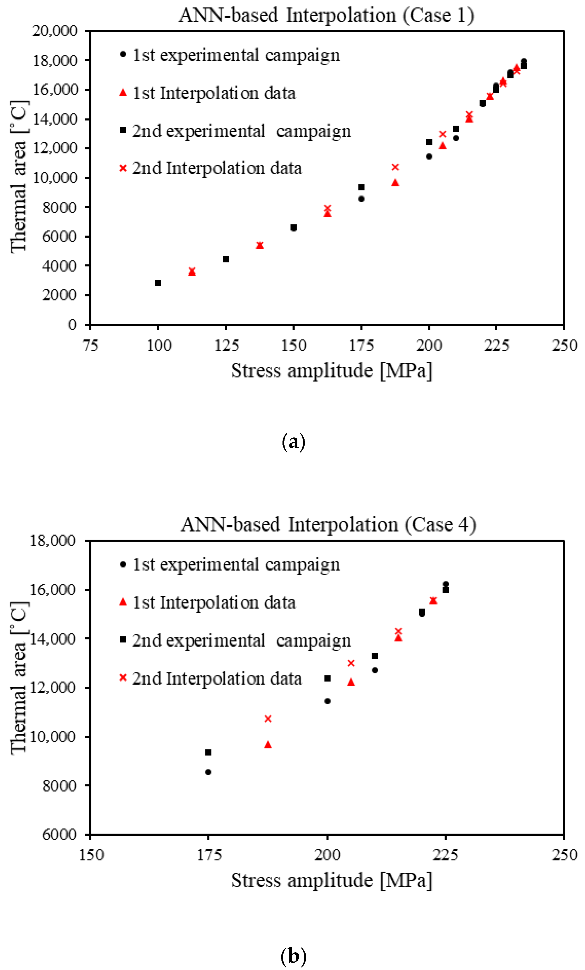
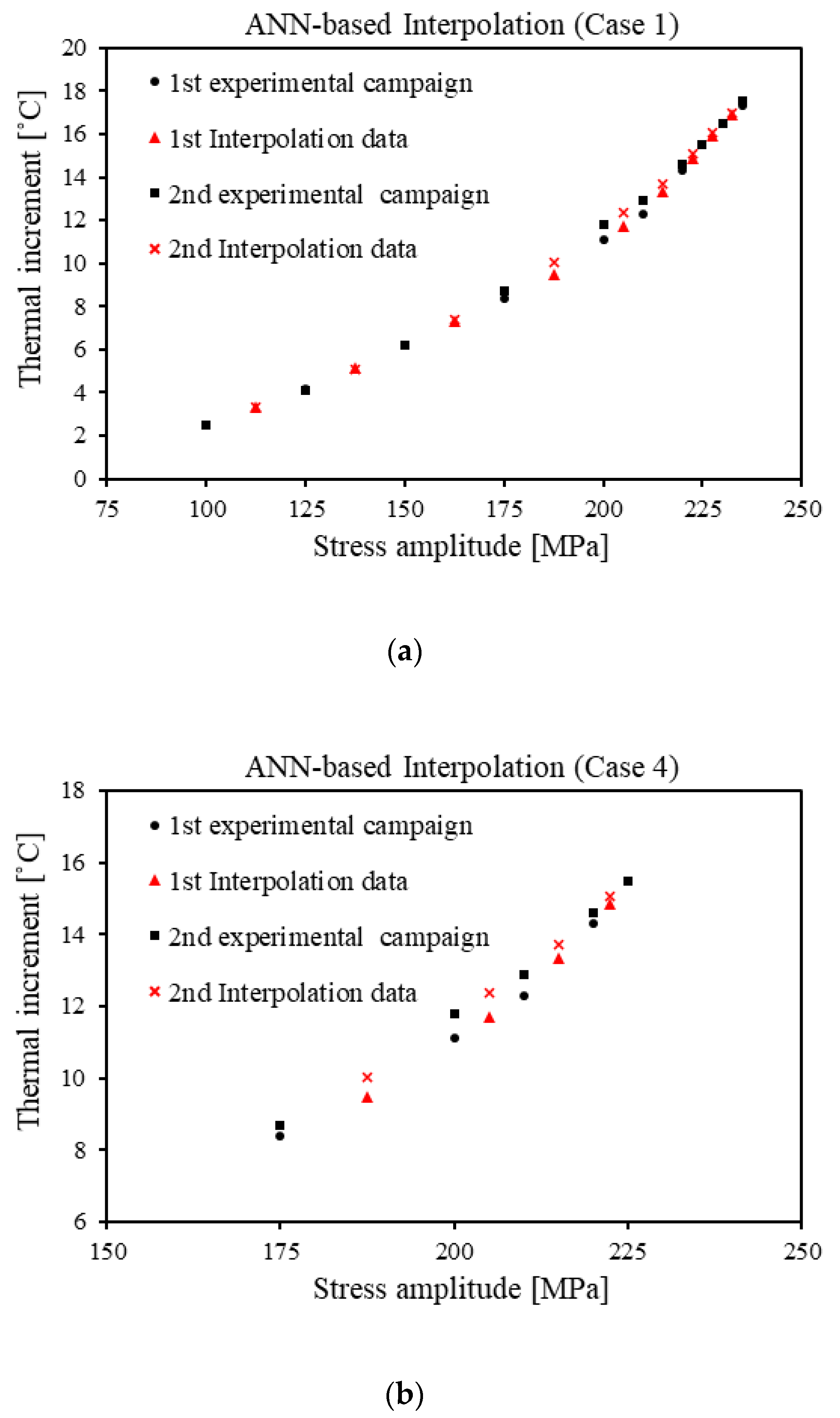
Once a new dataset selected from the original one was identified with a certain strategy, an augmented set of data was generated by using the ANN techniques (see Section 2.7). The strategy of ML interpolation can be an efficient way to streamline and increase the size of experimental datasets by reducing the cost and time involved in collecting more measurements. In this section, the interpolation method based on ANN is used to increase the accuracy and allow a more detailed assessment. By interpolating between the measured points, new values are obtained, so that a larger dataset and analysis can be performed. The higher the number of points, the more significant patterns and crucial trends can be identified. Figure 5 and Figure 6 show the results of the interpolation of thermal area and thermal increment for C45 steel using the ANN-based methods that are applied in this research. The solid curve is both the experimental data, and the interpolated values between experimental points are the intermediate ones. The intermediate (red points) showed interpolated values between the experimental points (black points).

3.1. ANN-Based Interpolation Accuracy

Table 4 shows the result of the accuracy metrics of the ANN-assisted interpolation for thermal parameters, the thermal area, and thermal increment methods, applied to C45. Based on this, the configuration is designed to be more accurate in interpolating the parameters. The interpolation of the experimental dataset (Case 1) reached RMSE 402 and 328 for thermal area and thermal increment, respectively, and R 2 0.99 on the C45 dataset, which implies smaller average and squared errors on the original response scale and justifies the selection of the other method. According to these metrics and the scope of the present dataset, the ANN provided a consistent interpolation of the experimental data.

3.2. Residual Analysis

Residuals between each experimental campaign ( y i ) and ANN-fitted value ( y ^ i ) at each stress level were computed ( e i = y i y ^ i ) for both thermal parameters. The relative error ( e i / y i ) was also reported [39,40].
The analysis is not aimed at any representation of predictive generalization, but as an in-domain consistency and spatial-bias test, because the ANN is applied in a manner that is an interpolation of values within the experimental stress range. The residuals varied around the zero across the stress range, and there are no apparent systematic signs of a tendency towards the fatigue limit area. This reveals no evident local bias by the ANN interpolation. Table 5 and Table 6 summarize the pointwise residual and the relative error for thermal area and thermal increment, respectively. In the two campaigns, the residuals of A and the ΔT are small at most stress levels. They also fluctuate around zero. This implies that the ANN fitting does not overestimate or underestimate the thermal parameters in a particular region of stress in a systematic manner. It is important to note that the trend of the residuals is not stable within the region of fatigue limit stress range. This would favour the application of the ANN curve as a numerical aid of interpolation to the subsequent TCM analysis.

3.3. TCM Using ANN-Augmented Datasets

Subsequently, the augmented dataset was utilised in the estimation of fatigue limits by means of the TCM, with various possibilities for approximating curves and thermal parameters taken into consideration. Finally, the results obtained from the TCM routine, testing the augmented dataset (Case 1, Case 2, Case 3, Case 4, and Case 5), are reported in Table 7 and compared with the results obtained from the original dataset (Case 0).
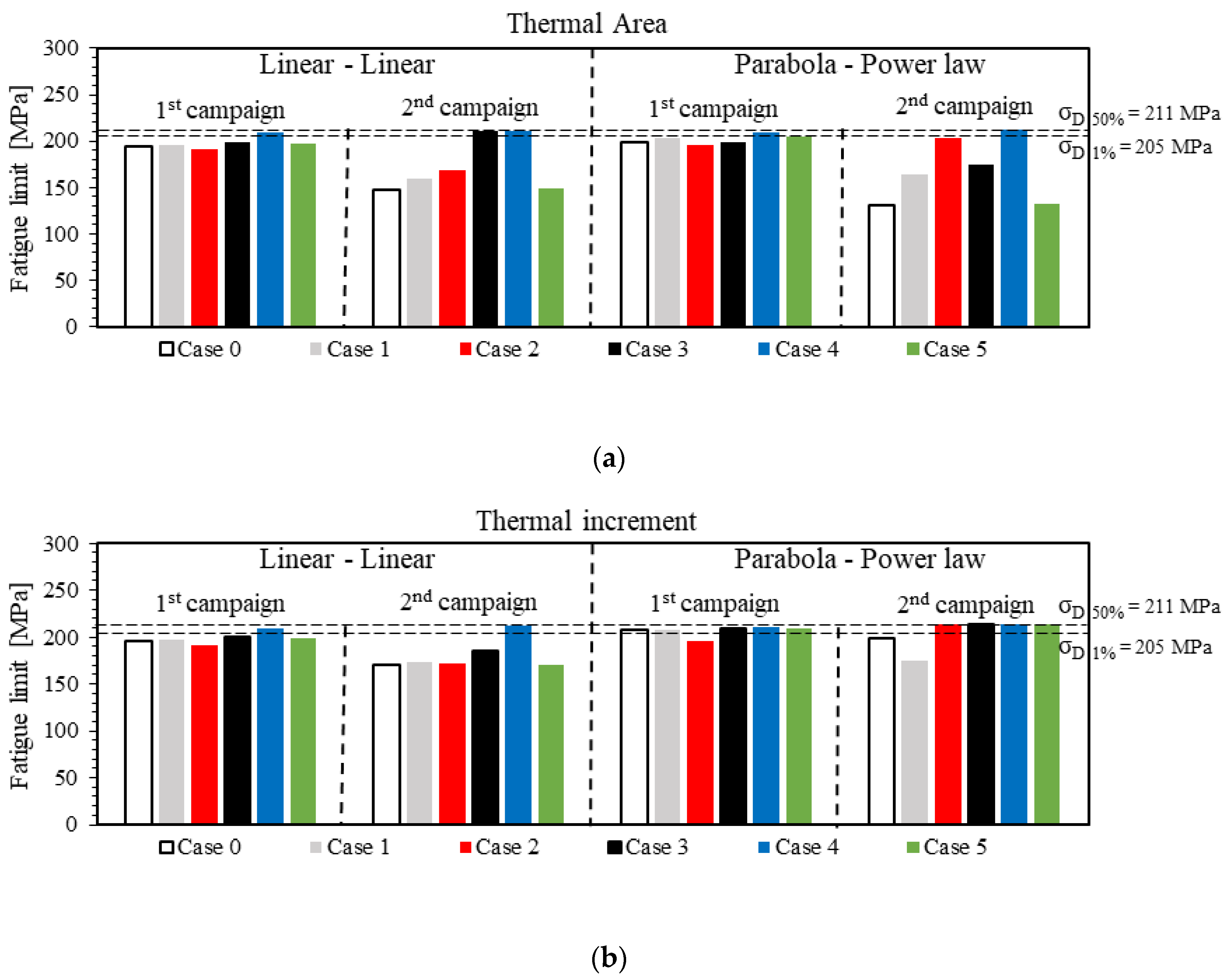
Table 7 presents a comparative analysis of fatigue limit values estimated by using the TCM routine. The strategies include configurations with and without (Case 0) ANN, varying the number and spatial distribution of measurement points (Case 1, Case 2, Case 3, Case 4, and Case 5). Two types of approximating curves are considered: linear–linear and parabola–power law, each assessed over two experimental campaigns (“1st” and “2nd”), with corresponding mean values, standard deviations, and deviations of each result from a central strategy reference corresponding to the Staircase Method (ΔTCM-SC). Furthermore, a representative value obtained from the two experimental campaigns was also reported in terms of mean value and the related standard deviation. The same results are graphically reported in Figure 7. The fatigue limit was estimated by studying the thermal area, A, and the thermal increment, ∆T, obtained from the TCM procedure and interpolated by ANN. Two appropriate fitting methods, linear–linear and parabola–power law, were considered, as shown in Figure 7. σ D , 50 % is the median staircase fatigue limit at which approximately half the specimens do not fail in the specified runout N cycles. In this study, it equals 211 MPa. The fatigue limit at 1% probability, denoted as σ D , 1 % , in this work is 205 MPa.
For the thermal area, the lowest fatigue limit was found for the second experimental campaign, when in this case, the TCM method was used without ANN interpolation in the linear–linear method, and the value was 148 MPa, and in the parabola–power law method, it was 131 MPa, as illustrated in Figure 7a. The best results in terms of the maximum and most accurate approximation were achieved for the second experimental campaign, where Case 3 and Case 4 were used in ANN, corresponding to σ D , 50 % , both equal to 211 MPa for the linear–linear TCM fitting technique. In the parabola–power law TCM technique, experimental campaigns resulted in 210 MPa and 212 MPa, respectively, for the Case 4 configuration, which was the best one. The worst result was offered by Case 5 and by Case 0, with 132 and 131 MPa, respectively.
The lowest fatigue limit was obtained using the Case 0 and Case 5 optimization strategies for the second campaign at 170 MPa. This is shown in Figure 7b, for the thermal increment, ∆T. The TCM technique was the linear–linear method. The optimum results (maximum and most accurate approximation) were obtained for the first and second experimental campaign, 209 and 212 MPa, respectively, for Cases 3 and 4, respectively. In the parabola–power law TCM method, the highest value of Case 2 was 214 MPa, which was obtained for the second campaign. Case 4 of the first campaign reached 210 MPa, which was close to σDSC−50%. The worst result was achieved with Case 2 at 196 MPa (Figure 7).

3.4. Uncertainty-Reduction Results

The repeatability-related uncertainty indicators for the investigated dataset-construction cases for both thermographic parameters, under the two fitting approaches (linear–linear and parabola–power law), are reported in Table 8. Because each case is available from two independent experimental campaigns, the analysis is focused on Type A repeatability within the investigated domain, quantified by the campaign-to-campaign spread R , the corresponding dispersion s , and the standard uncertainty of the mean u A . A lower R , s , or u A represents better agreement between campaigns and, therefore, less repeatability uncertainty.
For linear–linear, a clear reduction in uncertainty is seen as the construction of the dataset becomes more concentrated on the fatigue limit region. In particular, Case 4 reveals the greatest improvement for both of these parameters: u A is reduced from 23.0 to 1.0 MPa for A (UR approximately 95%) and from 12.5 to 1.5 MPa for ΔT (UR approximately 88%). This means that the Case 4 strategy provides the most consistent campaign-to-campaign estimates in the critical region related to fatigue limit determination. At the same time, the uncertainty reduction is not monotonic with respect to all strategies. Case 5 results in an increase in dispersion over the baseline (Case 0) with negative UR values for both thermal parameters. This confirms that the interpolation-assisted workflow is not a guarantee of improvement for any sampling strategy; the performance of the interpolation depends on how the dataset is constructed and where additional points are placed in the dataset.
For the parabola–power law, the behaviour is different in some cases. For the thermal area, uncertainty reduction is observed to be strong in cases built around the fatigue limit region, with Case 4 again resulting in the lowest dispersion ( u A = 1 MPa; UR about 97%). In contrast, for thermal increment, Cases 1 and 2 have significantly higher dispersion than the baseline, resulting in negative UR values. This means that, with this formulation of the fitting, the product of ΔT is more sensitive to the specific point placement (or the two-campaign variability) and can be less stable when the dataset is not built in an appropriate manner.
Overall, the results prove that the proposed interpolation-assisted workflow can mitigate the repeatability uncertainties when the construction of the dataset allows for a stable estimation in the vicinity of the fatigue limit region. It is worth noting Case 4 in particular. However, the fact that negative UR values are found in some cases shows that the improvement is not systematic but case-dependent. Practically, this implies that the strategy in the construction of the dataset is of at least the same importance as the choice of interpolator: the biggest advantage is gained when the additional points are placed in the region of stress that is most influential to the identification of the fatigue limit. Finally, it is important to clarify the extent of this uncertainty assessment. The metrics in Table 8 are from the within-domain, two-campaign repeatability Type A method. This method is not related to predictive uncertainty or generalization to new materials or loading conditions. This approach can be interpreted as an internal consistency check to support the robustness of this study’s dataset.

3.5. Case Comparison

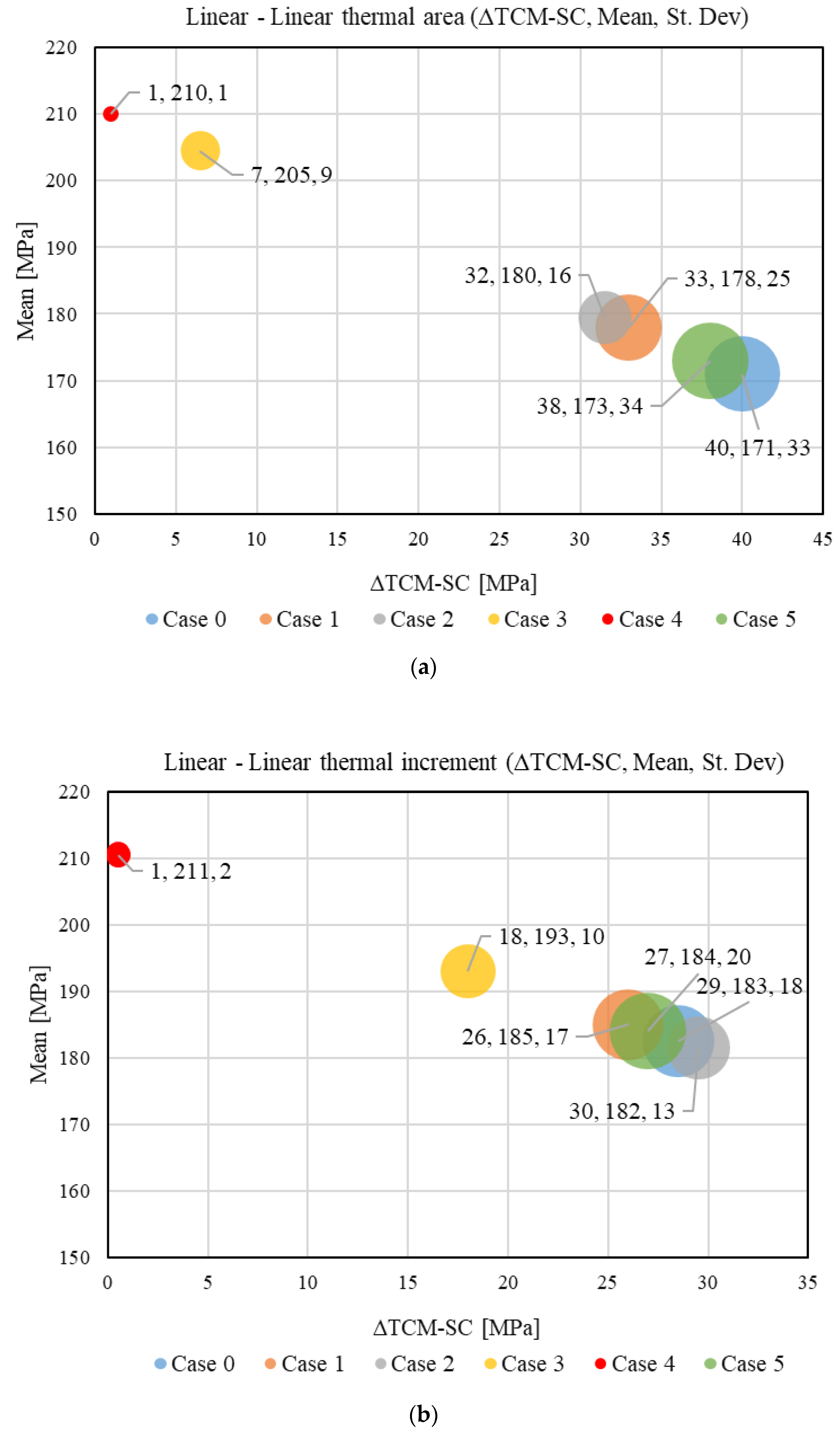
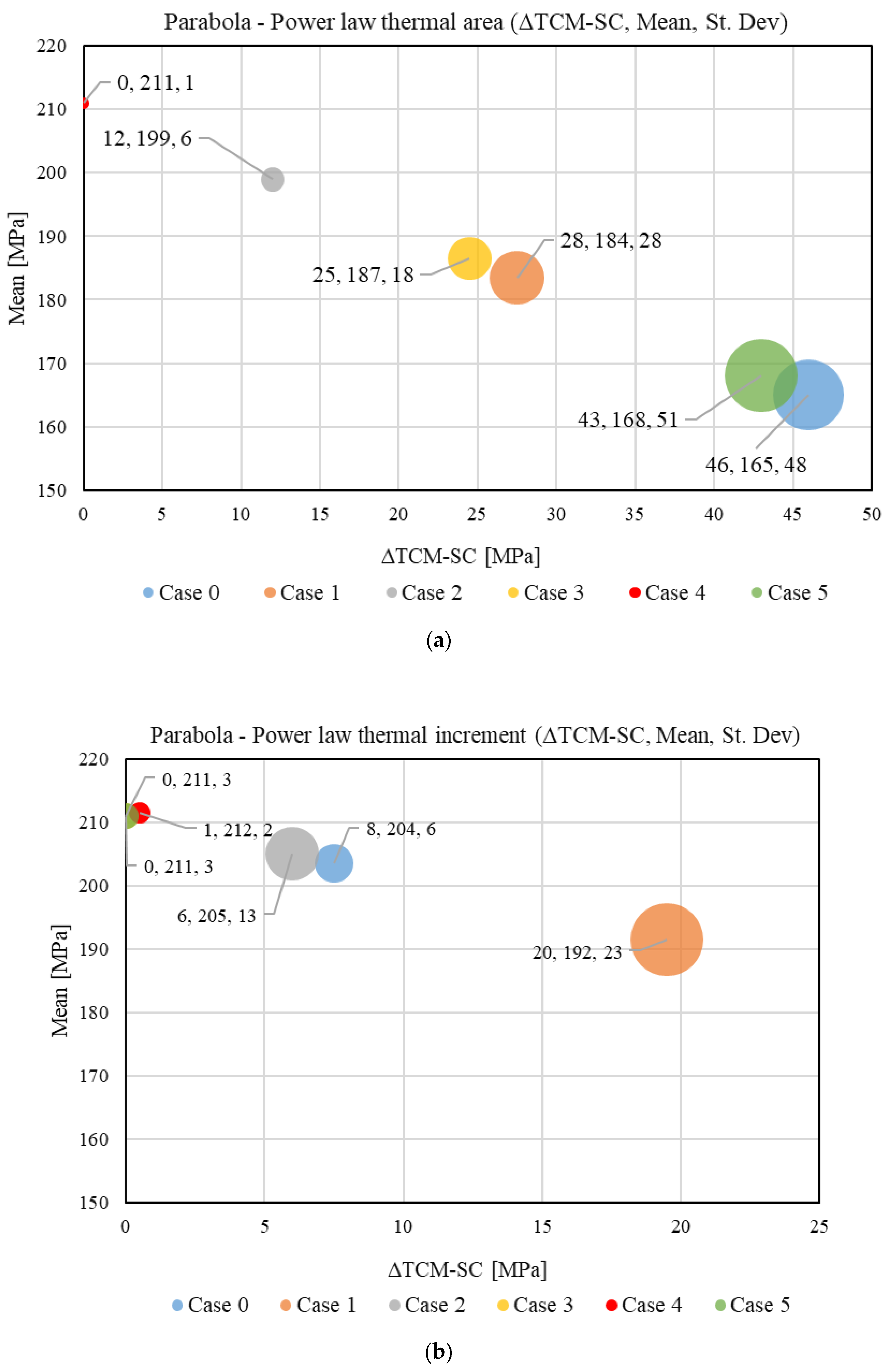
Figure 8 and Figure 9 show bubble plots for C45 in the linear–linear and parabola–power law methods. The horizontal axis is ΔTCM–SC in MPa, the vertical axis is the mean fatigue limit in MPa, and the bubble size is the standard deviation (St. Dev) of the two specimens. Points close to zero ΔTCM–SC and close to σ D , 50 % show better agreement with the staircase reference. Mean is the average of the fatigue limit for the two similar samples. St. Dev. is the standard deviation of those two estimates. ΔTCM–SC is the mean deviation from the staircase reference σ D , 50 % in MPa.
Figure 8a is for the thermal area of the linear–linear method plots, and Figure 8b is related to thermal increment. From Figure 7a, the fatigue limit of Case 4 is 210, and the standard deviation and DTCM-SC are 1, which is the best and most promising method. The worst method is for Figure 7a, Case 0, and for Figure 7b, Case 5.
Figure 9 is related to the parabola–power law approximation. In Figure 9a, the best is still Case 4, and the worst is Case 0. However, in the case of thermal increment (Figure 9b), the results are different. The difference between the fatigue limit and Case 3 and Case 5 is zero, and the difference between σ D , 50 % and Case 4 is only 1 MPa. The worst is Case 1. From the analysis of Figure 8 and Figure 9, it can be concluded that the optimised dataset, which had the capacity to minimise variations in the utilisation of various approximating curves (linear–linear and parabola–power law) and thermal parameters (thermal increment and thermal area), is Case 4. On the other hand, the optimised dataset in which an optimisation strategy involved the evolution of all thermal parameters (Case 1, Case 2, and Case 5) seemed to produce points in an area where optimisation is ineffective, affecting the overall estimation since the approximating curves were influenced in their evolution by these non-essential points. In Case 3, where the optimisation strategy was identical to that adopted for Case 4, the number of points selected as the initial starting point for optimisation using the ANN technique was increased by one compared to Case 4. This had a direct impact on the evolution of the thermal parameters immediately outside the transition zone. More in detail, the presence of points outside the transition zone led to a greater number of points outside the transition zone itself during optimisation, affecting the evolution of the approximating curves for estimating the fatigue resistance, similar to the effects observed in Cases 1, 2, and 5. Consequently, the optimisation of the original dataset based exclusively in the central zone, where the transition in the thermal parameters evolution is appreciable, is capable of producing repeatable results in the estimation. This observation was based on the estimation of the fatigue limit derived as the mean value of two distinct experimental campaigns.

4. Conclusions

The integration of ML techniques into the analysis of thermal parameter evolution has significantly enhanced the original datasets compared to those obtained through the initial experimental campaign. This improvement was reflected in reduced uncertainty among the use of different approximating curves for the fatigue limit estimation. As a matter of fact, the application of ML methods led to a notable decrease in variability among the approximating curves and the thermal parameters used in the analysis since the obtained results showed lower variance and more robust accuracy metrics. This way, precise determination of fatigue limits can be performed independently of the adopted approximating curves or thermal parameters.
Type-A repeatability uncertainty reduction, as indicated by lower variance and better measures of accuracy in the resultant TCM analysis, was attributable to the augmented datasets, especially those that were constructed around the central points near the fatigue limit (Cases 3 and 4). In such designs, the randomness of thermal response was greatly alleviated, and the ANN-assisted interpolation gave a more accurate account of the inherent dissipation trend with respect to stress amplitude.
According to the fatigue limit estimation perspective, the datasets optimized by ANN provided a significant decrease in the variability of the approximating curves and thermal parameters under consideration. In both linear–linear and parabola–power law TCM formulations, the optimal two-layer ANN-assisted configurations achieved fatigue limit values that were similar to those of the staircase reference ( σ D , 50 % = 211 MPa), and the ΔTCM–SC values were near zero and exhibited lower standard deviations compared to the original, non-interpolated datasets. This was the case with both thermal area and thermal increment, which demonstrated that the proposed strategy increases the strength of TCM-based fatigue limit estimation. It can be concluded that the optimal strategy for reducing variability in fatigue limit estimation when using different approximation curves and thermal parameters is to use an optimised dataset derived from optimising the evolution of thermal parameters, where the transition zone is appreciable from experimental data (Case 4).
Moreover, the developed methodology enabled a substantial reduction in the time required for the experimental campaign, improving the overall process of fatigue limit assessment. As a matter of fact, the proposed approach has the capacity to generate results with testing times reduced by up to 80% in comparison with those necessitated by the Staircase Method, since runout or failure conditions are not required. Furthermore, the analysis can be conducted using a small number of samples (only one or two), since the experimental campaign can be interrupted when the characteristic thermal parameter evolution occurs during fatigue testing, a scenario not applicable when using the Staircase Method, as a certain number of samples (generally 10 or more) is necessary for testing the failure and runout conditions.
These results show the potential of machine learning to optimize experimental workflows and improve the fidelity of material characterization in a new topic, such as the fatigue limit estimation by means of the Thermographic Method. In fact, even if this approach is widely adopted in the literature because the results are comparable to those provided when applying the Staircase Method, regardless of the analysis under consideration, the proposed study can further improve its application by reducing uncertainties in the estimation when adopting the Two-Curve Method for calculating the fatigue resistance. As a matter of fact, it is possible to conduct a series of experimental campaigns with a minimum of one or two samples for each case, with each analysis requiring approximately 10 tests as a starting point for defining the evolution of thermal parameters, offering significant advantages in terms of estimation and rapidity in the context of fatigue resistance assessments.

Author Contributions

Conceptualization, L.C. and M.D.A.; methodology, F.C.; software, M.S.J.; validation, M.D.A., L.C. and R.S.; formal analysis, L.C.; data curation, M.S.J.; writing—original draft preparation, L.C. and M.D.A.; writing—review and editing, L.C. and M.D.A.; visualization, M.S.J.; supervision, F.C. All authors have read and agreed to the published version of the manuscript.

Funding

This research received no external funding.

Data Availability Statement

The data presented in this study are available on request from the corresponding author due to privacy.

Conflicts of Interest

The authors declare no conflicts of interest.

References

  1. Maldague, X. Nondestructive evaluation of materials by infrared thermography. NDT E Int. 1996, 6, 396. [Google Scholar] [CrossRef]
  2. Doshvarpassand, S.; Wu, C.; Wang, X. An overview of corrosion defect characterization using active infrared thermography. Infrared Phys. Technol. 2019, 96, 366–389. [Google Scholar] [CrossRef]
  3. Attermo, R.; Östberg, G. Measurements of the temperature rise ahead of a fatigue crack. Int. J. Fract. Mech. 1971, 7, 122–124. [Google Scholar] [CrossRef]
  4. Luong, M.P. Infrared thermographic scanning of fatigue in metals. Nucl. Eng. Des. 1995, 158, 363–376. [Google Scholar] [CrossRef]
  5. Curti, G.; Geraci, A.; Risitano, A. Un nuovo metodo per la determinazione rapida del limite di fatica. ATA 1989, 10, 634–636. [Google Scholar]
  6. BS ISO 12107:2003; Metallic Materials: Fatigue Testing: Statistical Planning and Analysis of Data. ISO: Geneva, Switzerland, 2003.
  7. La Rosa, G.; Risitano, A. Thermographic methodology for rapid determination of the fatigue limit of materials and mechanical components. Int. J. Fatigue 2000, 22, 65–73. [Google Scholar] [CrossRef]
  8. Fargione, G.; Geraci, A.; La Rosa, G.; Risitano, A. Rapid determination of the fatigue curve by the thermographic method. Int. J. Fatigue 2002, 24, 11–19. [Google Scholar] [CrossRef]
  9. Curà, F.; Curti, G.; Sesana, R. A new iteration method for the thermographic determination of fatigue limit in steels. Int. J. Fatigue 2005, 27, 453–459. [Google Scholar] [CrossRef]
  10. Curà, F.; Gallinatti, A.E.; Sesana, R. Dissipative aspects in thermographic methods. Fatigue Fract. Eng. Mater. Struct. 2012, 35, 1133–1147. [Google Scholar] [CrossRef]
  11. Mahmoudi, A.; Khonsari, M.M. Rapid evaluation of fatigue limit using energy dissipation. Fatigue Fract. Eng. Mater. Struct. 2023, 46, 2156–2167. [Google Scholar] [CrossRef]
  12. Stergiou, K.; Ntakolia, C.; Varytis, P.; Koumoulos, E.; Karlsson, P.; Moustakidis, S. Enhancing property prediction and process optimization in building materials through machine learning: A review. Comput. Mater. Sci. 2023, 220, 112031. [Google Scholar] [CrossRef]
  13. Basheer, I.A.; Hajmeer, M. Artificial neural networks: Fundamentals, computing, design, and application. J. Microbiol. Methods 2000, 43, 3–31. [Google Scholar] [CrossRef]
  14. Opěla, P.; Schindler, I.; Kawulok, P.; Kawulok, R.; Rusz, S.; Navrátil, H. On various multi-layer perceptron and radial basis function based artificial neural networks in the process of a hot flow curve description. J. Mater. Res. Technol. 2021, 14, 1837–1847. [Google Scholar] [CrossRef]
  15. Tize Mha, P.; Dhondapure, P.; Jahazi, M.; Tongne, A.; Pantalé, O. Interpolation and Extrapolation Performance Measurement of Analytical and ANN-Based Flow Laws for Hot Deformation Behavior of Medium Carbon Steel. Metals 2023, 13, 633. [Google Scholar] [CrossRef]
  16. Kebede, H.; Demissie, Z.; Tadesse, H.; Eshetu, A. Spatial interpolation techniques comparison and evaluation: The case of ground-based gravity and elevation datasets of the central Main Ethiopian rift. Heliyon 2024, 10, e32806. [Google Scholar] [CrossRef] [PubMed]
  17. Liu, H.; Yu, H.; Guo, C.; Chen, X.; Zhong, S.; Zhou, L.; Osman, A.; Lu, J. Review on Fatigue of Additive Manufactured Metallic Alloys: Microstructure, Performance, Enhancement, and Assessment Methods. Adv. Mater. 2024, 36, 2306570. [Google Scholar] [CrossRef]
  18. Park, C.; Saha, S.; Guo, J.; Zhang, H.; Xie, X.; Bessa, M.A.; Qian, D.; Chen, W.; Wanger, G.J.; Cao, J.; et al. Unifying machine learning and interpolation theory via interpolating neural networks. Nat. Commun. 2025, 16, 8753. [Google Scholar] [CrossRef] [PubMed]
  19. Bučar, T.; Nagode, M.; Fajdiga, M. A neural network approach to describing the scatter of S–N curves. Int. J. Fatigue 2006, 28, 311–323. [Google Scholar] [CrossRef]
  20. Marković, E.; Marohnić, T.; Basan, R. A Surrogate Artificial Neural Network Model for Estimating the Fatigue Life of Steel Components Based on Finite Element Simulations. Materials 2025, 18, 2756. [Google Scholar] [CrossRef]
  21. Srinivasan, D.V.; Moradi, M.; Komninos, P.; Zarouchas, D.; Vassilopoulos, A.P. A generalized machine learning framework to estimate fatigue life across materials with minimal data. Mater. Des. 2024, 246, 113355. [Google Scholar] [CrossRef]
  22. Yuan, K.; Peng, S.; Sun, Z. An artificial neural network model for fatigue damage analysis of wide-band non-Gaussian random processes. Appl. Ocean Res. 2024, 144, 103896. [Google Scholar] [CrossRef]
  23. Fernández, J.; Chiachío, M.; Chiachío, J.; Muñoz, R.; Herrera, F. Uncertainty quantification in Neural Networks by Approximate Bayesian Computation: Application to fatigue in composite materials. Eng. Appl. Artif. Intell. 2022, 107, 104511. [Google Scholar] [CrossRef]
  24. Corsaro, L. Passive and Active Thermography for Surface Treatments Characterization in Spur Gears; Politecnico di Torino: Torino, Italy, 2024. [Google Scholar]
  25. Qian, H.; Zheng, J.; Wang, Y.; Jiang, D. Fatigue Life Prediction Method of Ceramic Matrix Composites Based on Artificial Neural Network. Appl. Compos. Mater. 2023, 30, 1251–1268. [Google Scholar] [CrossRef]
  26. Corsaro, L.; Dehghanpour Abyaneh, M.; Curà, F.; Sesana, R. Thermographic and Machine Learning approaches for a rapid estimation of gears bending fatigue strength. Forsch. Im Ingenieurwesen 2025, 89, 122. [Google Scholar] [CrossRef]
  27. Ehteshamfar, M.V.; Javadi, M.S.; Adibi, H. Surface modification of prototypes in fused deposition modelling using lapping process. Rapid Prototyp. J. 2022, 28, 1382–1393. [Google Scholar] [CrossRef]
  28. Dehghanpour Abyaneh, M.; Narimani, P.; Javadi, M.S.; Golabchi, M.; Attarsharghi, S.; Hadad, M. Predicting Surface Roughness and Grinding Forces in UNS S34700 Steel Grinding: A Machine Learning and Genetic Algorithm Approach to Coolant Effects. Physchem 2024, 4, 495–523. [Google Scholar] [CrossRef]
  29. Javadi, M.S.; Ehteshamfar, M.V.; Adibi, H. A comprehensive analysis and prediction of the effect of groove shape and volume fraction of multi-walled carbon nanotubes on the polymer 3D-printed parts in the friction stir welding process. Polym. Test. 2023, 117, 107844. [Google Scholar] [CrossRef]
  30. Hodson, T.O. Root-mean-square error (RMSE) or mean absolute error (MAE): When to use them or not. Geosci. Model Dev. 2022, 15, 5481–5487. [Google Scholar] [CrossRef]
  31. Azarafza, M.; Hajialilue Bonab, M.; Derakhshani, R. A Deep Learning Method for the Prediction of the Index Mechanical Properties and Strength Parameters of Marlstone. Materials 2022, 15, 6899. [Google Scholar] [CrossRef]
  32. Chai, T.; Draxler, R.R. Root mean square error (RMSE) or mean absolute error (MAE)?—Arguments against avoiding RMSE in the literature. Geosci. Model Dev. 2014, 7, 1247–1250. [Google Scholar] [CrossRef]
  33. Cheng, H.; Garrick, D.J.; Fernando, R.L. Efficient strategies for leave-one-out cross validation for genomic best linear unbiased prediction. J. Anim. Sci. Biotechnol. 2017, 8, 38. [Google Scholar] [CrossRef] [PubMed]
  34. Cheng, J.; Dekkers, J.C.M.; Fernando, R.L. Cross-validation of best linear unbiased predictions of breeding values using an efficient leave-one-out strategy. J. Anim. Breed. Genet. 2021, 138, 519–527. [Google Scholar] [CrossRef] [PubMed]
  35. Geroldinger, A.; Lusa, L.; Nold, M.; Heinze, G. Leave-one-out cross-validation, penalization, and differential bias of some prediction model performance measures—A simulation study. Diagn. Progn. Res. 2023, 7, 9. [Google Scholar] [CrossRef] [PubMed]
  36. Bartlett, J.W.; Frost, C. Reliability, repeatability and reproducibility: Analysis of measurement errors in continuous variables. Ultrasound Obstet. Gynecol. 2008, 31, 466–475. [Google Scholar] [CrossRef]
  37. Jcgm, J. Evaluation of measurement data—Guide to the expression of uncertainty in measurement. Int. Organ. Stand. Geneva ISBN 2008, 50, 134. [Google Scholar]
  38. De Bièvre, P. The 2007 International Vocabulary of Metrology (VIM), JCGM 200: 2008 [ISO/IEC Guide 99]: Meeting the need for intercontinentally understood concepts and their associated intercontinentally agreed terms. Clin. Biochem. 2009, 42, 246–248. [Google Scholar] [CrossRef]
  39. Hastie, T.; Tibshirani, R.; Friedman, J. The Elements of Statistical Learning; Springer: Berlin/Heidelberg, Germany, 2009. [Google Scholar]
  40. James, G.; Witten, D.; Hastie, T.; Tibshirani, R. Linear Model Selection and Regularization. In An Introduction to Statistical Learning: With Applications in R; James, G., Witten, D., Hastie, T., Tibshirani, R., Eds.; Springer: New York, NY, USA, 2021; pp. 225–288. [Google Scholar]
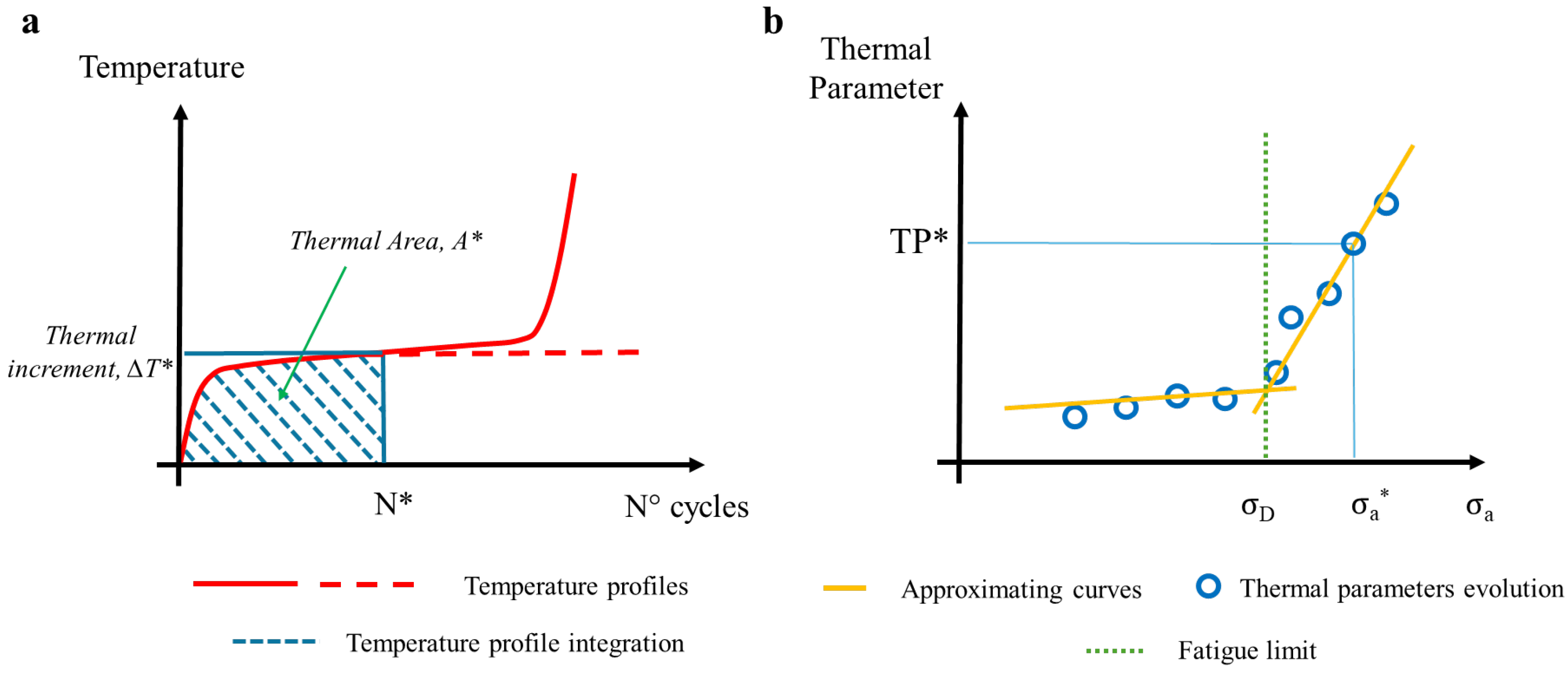
Figure 1. (a) Thermal profile; (b) fatigue limit estimation.
Metals 16 00042 g001
Figure 2. Cylindrical sample for fatigue tests.
Metals 16 00042 g002
Figure 3. Experimental trend for the Staircase Method application.
Metals 16 00042 g003
Figure 4. ANN architecture feed-forward with interpolation.
Metals 16 00042 g004
Figure 5. C45 steel ANN-interpolation of thermal area: (a) Case 1; (b) Case 4.
Metals 16 00042 g005
Figure 6. C45 steel ANN-interpolation of thermal increment: (a) Case 1; (b) Case 4.
Metals 16 00042 g006
Figure 7. Comparison of fatigue limits obtained from TCM methods for (a) thermal area; (b) thermal increment.
Metals 16 00042 g007
Figure 8. Bubble plot comparison of linear–linear TCM results for (a) thermal area; (b) thermal increment.
Metals 16 00042 g008
Figure 9. Bubble plot comparison of parabola–power law TCM results for (a) thermal area; (b) thermal increment.
Metals 16 00042 g009
Table 1. An overview of the available literature that uses ML methods for fatigue modelling.
Ref.MaterialModelDomain/DatasetInterpolation
[18]MethodologyINNMethod theoryYes
[19]MetalsMLPS-N datasets/ExperimentsYes
[20]SteelANNFatigue life/FE-generatedIn range 1
[21]Polymers and AM MLFatigue life/ExperimentsNo
[22]MetalsANNNon-Gaussian loading/ExperimentsNo
[23]CompositesBNNFatigue life/Experiments (UQ)No
This studyC45 steelANNThermal parameters/ExperimentsYes
1 Predictions stayed inside the tested domain without doing explicit curve interpolation.
Table 2. Experimental fatigue characterization.
Staircase Method PT Approach (TCM)
50%
probability
1%
probability
Approximating curvesThermal parameters1st experimental
campaign
2nd experimental
campaign
σ D , 50 %
[MPa]
σ D , 1 % [MPa]σDTCM-1 [MPa]σDTCM-2 [MPa]
211205Parabola–power lawΔT208199
A199131
Linear–linearΔT195170
A194148
Table 3. Optimal configuration and performance of the ANN interpolation model.
ParameterRangeValue
Hidden layers(16), (32), (64), (32, 16), (64, 32), (128, 64)(128, 64)
Alpha (L2)1 × 10⁻², 3 × 10⁻³, 1 × 10⁻³, 3 × 10⁻⁴, 1 × 10⁻⁴, 1 × 10⁻⁵, 1 × 10−60.0001
Activation-ReLU
Solver-Adam
Learning rate (init)-0.01
Table 4. Accuracy metrics for C45 using ANN interpolation.
Thermal Parameters M S E R M S E R 2 M A E
A [°C]162,181.46402.710.99330.48
ΔT [°C]108,034.41328.680.99265.12
Table 5. Residual analysis for thermal area.
Stress
Amplitude [MPa]
1st
Campaign
ANN FitResidualRelative Error [%]2nd
Campaign
ANN FitResidualRelative Error [%]
1002,846.92,846.80.0960.0032,856.82,849.097.7100.269
1254,4584,458.23−0.2270.0054,482.84,489.58−6.7760.151
1506,5646,563.930.0720.0016,626.86,626.270.5270.007
1758,573.18,573.15−0.0530.0009,361.79,357.394.3110.046
20011,452.911,452.80.1400.00112,397.312,395.71.5700.012
21012,712.613,091.8−379.2002.98313,314.913,560.1−245.1501.841
22015,03715,038.5−1.4900.00915,111.415,157.4−45.9700.304
22516,244.116,101.2142.9300.87915,987.716,012.8−25.1200.157
23017,165.917,163.82.0700.012016,990.316,868.2122.1100.718
23517,927.917,928.5−0.5900.00317,590.417,664.6−74.2400.422
Table 6. Residual analysis for thermal increment.
Stress
Amplitude [MPa]
1st
Campaign
ANN FitResidualRelative Error [%]2nd
Campaign
ANN FitResidualRelative Error [%]
1002.52.4650.0351.4002.52.4770.0220.883
1254.24.242−0.0421.0054.14.137−0.0370.919
1506.26.1810.0180.3056.26.1780.0210.353
1758.48.3990.0000.0058.78.6990.0000.002
20011.111.0950.0040.04011.811.7900.0090.082
21012.312.421−0.1210.98712.913.002−0.1020.792
22014.314.338−0.0380.26814.614.5910.0080.056
22515.515.3720.1270.82415.515.553−0.0530.342
23016.516.4060.0940.56916.516.514−0.0140.088
23517.317.375−0.0750.43417.517.4760.0230.136
Table 7. The result of TCM methods for different strategies.
TCM MethodsExperimental CampaignCase 0Case 1Case 2Case 3Case 4Case 5
Approximating Curves ΔTAΔTAΔTAΔTAΔTAΔTA
Linear–linear1st195194197196191191200198209209198197
2nd170148173160172168186211212211170149
Mean183171185178182180193205211210184173
St. Dev183317251316109212034
∆TCM-SC294026333032187112738
Parabola–power law1st208199208203196195209199210210209204
2nd199131175164214203213174213212213132
Mean204165192184205199211187212211211168
St. Dev648232813631821351
∆TCM-SC846202861202510043
Table 8. Uncertainty reduction summary across cases.
Thermal Area (A)Thermal Increment (ΔT)
Approximating CurvesCase R s u A UR vs. Case 0 R s u A UR vs. Case 0
Linear–linearCase 04632.5323.00.00%2517.6812.50.00%
Case 13625.4618.021.74%2416.9712.04.00%
Case 22316.2611.550.00%1913.449.524.00%
Case 3139.196.571.74%149.907.044.00%
Case 421.411.095.65%32.121.588.00%
Case 54833.9424.0−4.35%2819.8014.0−12.00%
Parabola–power lawCase 06848.0834.00.00%96.364.50.00%
Case 13927.5819.542.65%3323.3316.5−266.67%
Case 285.664.088.24%1812.739.0−100.00%
Case 32517.6812.563.24%42.832.055.56%
Case 421.411.097.06%32.121.566.67%
Case 57250.9136.0−5.88%42.832.055.56%
Disclaimer/Publisher’s Note: The statements, opinions and data contained in all publications are solely those of the individual author(s) and contributor(s) and not of MDPI and/or the editor(s). MDPI and/or the editor(s) disclaim responsibility for any injury to people or property resulting from any ideas, methods, instructions or products referred to in the content.