Article

A Simulation-Based Comparative Analysis of Physics and Data-Driven Models for Temperature Prediction in Steel Coil Annealing

Institute of Control and Informatization of Production Processes, Faculty BERG, Technical University of Košice, Němcovej 3, 04200 Košice, Slovakia
*
Author to whom correspondence should be addressed.
Metals 2025, 15(9), 932; https://doi.org/10.3390/met15090932
Submission received: 18 July 2025 / Revised: 19 August 2025 / Accepted: 20 August 2025 / Published: 22 August 2025

Abstract

Annealing of steel coils in bell-type furnaces is a critical process in steel production, requiring precise temperature control to ensure desired mechanical properties and microstructure. However, direct measurement of inner coil temperatures is impractical in industrial conditions, necessitating model-based estimation. This study presents a comparative analysis of physics-based and machine learning (ML) approaches for predicting internal temperatures during annealing. A finite difference method (FDM) was developed as a physics-based model and validated against experimental data from both laboratory and industrial annealing cycles. Furthermore, several ML models, including support vector regression (SVR), neural networks (NN), multivariate adaptive regression splines (MARS), k-nearest neighbors (k-NN), and random forests (RFs), were trained on surface temperature measurements to predict inner temperatures. The results demonstrate that the MARS, k-NN, and RF models achieved high prediction accuracy with performance index (PI) values below 1.0 on unseen data, demonstrating excellent generalization capabilities. In contrast, SVR with polynomial kernels and NN exhibited poor performance in specific configurations, highlighting their sensitivity to overfitting and data variability. The findings suggest that combining physics-based models with data-driven techniques offers a robust framework for soft-sensing in annealing operations, enabling improved process monitoring and control.

1. Introduction

Annealing of steel coils in bell-type furnaces is a critical heat treatment process aimed at restoring the ductility and mechanical properties of cold-rolled steel through recrystallization. During cold rolling, steel undergoes significant plastic deformation, which leads to work hardening and increased internal stresses. Recrystallization annealing serves to eliminate these effects by heating the material to a temperature at which new, strain-free grains form, thereby improving formability and reducing residual stresses.
The competitiveness of a steel production company is strongly influenced by the quality and cost efficiency of its products. In the context of annealing processes, the temperature distribution within steel coils plays a key role in determining both product quality and overall energy consumption. Excessively high temperatures lead to unnecessary energy costs, while insufficient heating can result in products that do not meet quality requirements. Although various sensors are available for measuring the surface temperature of steel coils, the internal temperature cannot be measured directly without damaging the material. Therefore, model-based soft sensors are essential for estimating internal temperature values. These soft sensors make it possible to monitor and control the temperature behavior of the material in real time, even in processes characterized by significant time delays.
In industrial practice, bell-type annealing furnaces are widely used due to their flexibility and suitability for batch processing of coiled steel. Each annealing cycle involves controlled heating, holding at the target temperature, and subsequent cooling, all of which must be carefully managed to ensure uniform microstructural transformation throughout the coil volume. However, due to the considerable thermal mass and layered geometry of steel coils, temperature gradients often develop between the outer and inner layers, significantly influencing the kinetics of recrystallization.
Accurate knowledge of the temperature distribution within the steel coil is essential not only for ensuring product quality but also for optimizing furnace operation and energy consumption. In practice, the internal coil temperature is not directly measurable during each annealing cycle, as embedding thermocouples into every coil is impractical and economically unfeasible. As a result, furnace operators often rely on empirical rules and accumulated experience to manage the process, which can lead to conservative heating strategies and suboptimal fuel usage.
To address this limitation, mathematical models capable of estimating the internal temperature evolution in real time have been developed. Such models support better control strategies, reduce unnecessary fuel consumption, and improve process repeatability. Traditional approaches are based on the solution of the unsteady heat conduction equation, typically the one-dimensional Fourier heat equation, with appropriate boundary and initial conditions tailored to the geometry of coiled steel.
More recently, data-driven techniques based on machine learning (ML) have emerged as promising alternatives or complements to physics-based models. Methods such as support vector regression (SVR), multivariate adaptive regression splines (MARS), neural networks (NNs), and random forests (RF) can capture complex thermal dynamics from historical process data without requiring detailed knowledge of material properties or furnace configurations.
The modeling and prediction of temperature inside steel coils during annealing in bell-type furnaces represent a complex technological challenge at the intersection of heat transfer science, process control, and artificial intelligence. Accurate temperature prediction is essential for ensuring metallurgical quality, energy optimization, and real-time process control. Here, we systematically analyze the current state-of-the-art, spanning traditional mathematical models through contemporary machine learning (ML) approaches, and provide a comparison of their performance and applicability.
This study presents the theoretical foundation for soft-sensor modeling and evaluates the proposed models using data from laboratory measurements and real industrial operations. The objective was to develop a soft-sensor model capable of estimating internal coil temperatures from surface temperature measurements. For validation purposes, thermocouples were used to measure inner temperatures during selected annealing cycles.
This article presents a comparative study of temperature prediction methods for the annealing of steel coils in bell-type furnaces. We begin by formulating a physical model based on the transient Fourier heat conduction equation and validating it against available data. Subsequently, we introduce several machine learning techniques trained on recorded furnace data and evaluate their performance in predicting internal coil temperatures. The aim is to highlight the trade-offs between physical interpretability, prediction accuracy, and operational usability of the various approaches.
In previous work, the authors developed methods for soft-sensing surface temperatures of steel coils based on the temperature of the annealing atmosphere in a bell-type furnace [1,2]. In addition to this, a second approach focused on the estimation of internal coil temperatures was partially verified using machine learning techniques, specifically support vector regression (SVR), a form of support vector machines (SVMs) [3].
This study continues from previous research to analyze other ML methods like multivariate adaptive regression splines (MARS), neural networks (NNs), and random forests (RFs), which were employed.
The results obtained from these black-box machine learning models are compared in this paper with those derived from an analytical model based on heat conduction theory. The proposed approaches are intended for potential use in online estimation of internal temperatures, thereby enabling better monitoring and control of the annealing process. This paper presents both experimental data and simulation results to validate the proposed methods.
This study addresses the critical challenge of accurately estimating internal temperatures during annealing using surface measurements. While various machine learning methods have been applied in different metallurgical processes, their use for real-time prediction of internal strip temperatures based on operational data remains limited. The novelty of this work lies in the comprehensive comparison of physics-based and multiple machine learning models under both laboratory and industrial conditions. The proposed workflow integrates experimental measurements, preprocessing, model training, and evaluation, offering a practical solution for enhancing soft-sensing capabilities in annealing operations. By evaluating the generalization capabilities of each model on real unseen data, this study contributes valuable insights into the selection and deployment of predictive models in metallurgical practice.
Common abbreviations are listed at the end of the paper.

2. Review of the Related Literature

Recent research has addressed various aspects of annealing processes and their influence on the microstructure and properties of steels. Couchet et al. [4] conducted a numerical investigation of phase transformations during intercritical annealing, incorporating interface thermodynamic conditions into their simulations, which provides a relevant framework for thermal cycle modeling in steel coils. Yang et al. [5] examined the effect of annealing temperature on the microstructure and mechanical properties of DH steel, optimizing hole expansion properties through precise control of thermal parameters. Similarly, Chu et al. [6] studied the evolution of microstructure, mechanical performance, and fracture behavior of complex-phase steels across different annealing temperatures, offering valuable insights into linking temperature profiles to material behavior.
Steel strip annealing is commonly performed in two ways: batch annealing, where coiled strips are processed in bell-type furnaces, and continuous annealing, in which strips pass through a furnace line. Many studies have addressed temperature evolution in these processes, as it strongly influences the final mechanical properties. Modeling approaches fall broadly into physics-based and data-driven categories, with recent work focusing on hybrid strategies that integrate both.

2.1. Physics-Based Modeling Approaches

Finite difference and finite element methods (FDM/FEM) discretize transient heat conduction equations based on Fourier’s law to simulate temperature fields in coils. These models capture conduction, convection, and radiation effects, and have been validated with industrial data for process optimization [7,8]. Examples include intelligent soft-sensing systems for internal coil temperature [9,10] and simplified heat-flow models for surface temperature estimation [1]. Lumped parameter models (LPMs) approximate the coil as uniform thermal masses, trading spatial resolution for computational speed, making them suitable for real-time prediction [8]. Hybrid approaches combine physical equations with parameter tuning derived from measurements, thereby improving adaptability while maintaining interpretability [11,12,13]. Durdán et al. [2] and Kostúr [14] introduced a soft-sensing approach that estimates internal and surface coil temperatures based on the protective atmosphere’s temperature, as measured by thermocouples. Their system uses unsteady heat conduction models and is validated against operational data from an annealing plant. In their methodology, surface temperature is predicted using a regression model, while the inner temperature is estimated via differential equations.

2.2. Machine Learning and Data-Driven Methods

The integration of data-driven approaches into steel processing has also gained increasing attention. Zhou et al. [15] applied machine learning techniques for composition design of high-yield-strength TWIP steels, demonstrating the potential of AI-based tools in optimizing input parameters for predictive models. Bachmann et al. [16] proposed reproducible quantification of complex steel microstructures using advanced machine learning methods, enabling improved material characterization for simulation purposes. Tiwari et al. [17] developed artificial neural network models to predict the mechanical properties of industrial C–Mn cast steels, confirming that AI-based methods can complement physics-based models in steel property prediction.
Artificial neural networks (ANNs) and related models have been trained on process data to capture nonlinear relations between furnace parameters and coil temperature [18,19,20]. Various applications of neural networks in annealing can be found in [21,22,23,24,25,26,27]. Applications include batch and continuous annealing, with methods ranging from backpropagation to generalized regression neural networks [28,29,30]. While flexible, these models risk overfitting and require careful training/validation [21,25,26]. Ensemble learning and incremental updates improve robustness and adaptability [19]. Support Vector Regression (SVR) has also been explored for furnace temperature prediction and process optimization [31,32,33]. Bayesian methods offer uncertainty quantification in predictions [34].

2.3. Trends and Synthesis

Recent trends emphasize hybridization of physics-based and ML models, computational feasibility for online control, robust learning for noisy industrial data, and adaptability through model updating [8,35]. These developments align with the move towards digital twins in annealing operations. A concise comparison of physics-based, machine learning, and hybrid modeling approaches is provided in Appendix A (see Table A1). This table summarizes the main approaches for temperature modeling in steel coil annealing. Reviews by Smith and Yates [36] and Łach and Svyetlichnyy [37] summarize modern hybrid strategies that combine PDE-based models with machine learning components, providing improved accuracy, interpretability, and computational efficiency in heat transfer simulations.

3. Understanding Steel Coil Annealing

Bell-type furnaces are widely used for annealing steel coils, such as strips or wires, and can be heated electrically or by fuel. They are applicable for various heat treatments up to 1100 °C (Figure 1) [38]. The furnace consists of a fixed base with a cylindrical heating hood, inner muffle, convection rings, and burners or catalytic pads for efficient, low-emission heating [39,40].
During annealing, the steel is heated above the recrystallization temperature to improve ductility and reduce hardness [38,41]. The process involves recovery, recrystallization, and grain growth [42,43]. Coils are stacked in layers, covered with an inert gas to avoid oxidation, and heated tangentially via the inner cover. Due to the coil’s thermal mass, heating, holding, and cooling stages are prolonged to ensure uniform temperature distribution [44].
Figure 2 shows a typical batch annealing cycle. Recrystallization generally starts around 550 °C and its progression depends on both temperature and atmosphere [41,45].
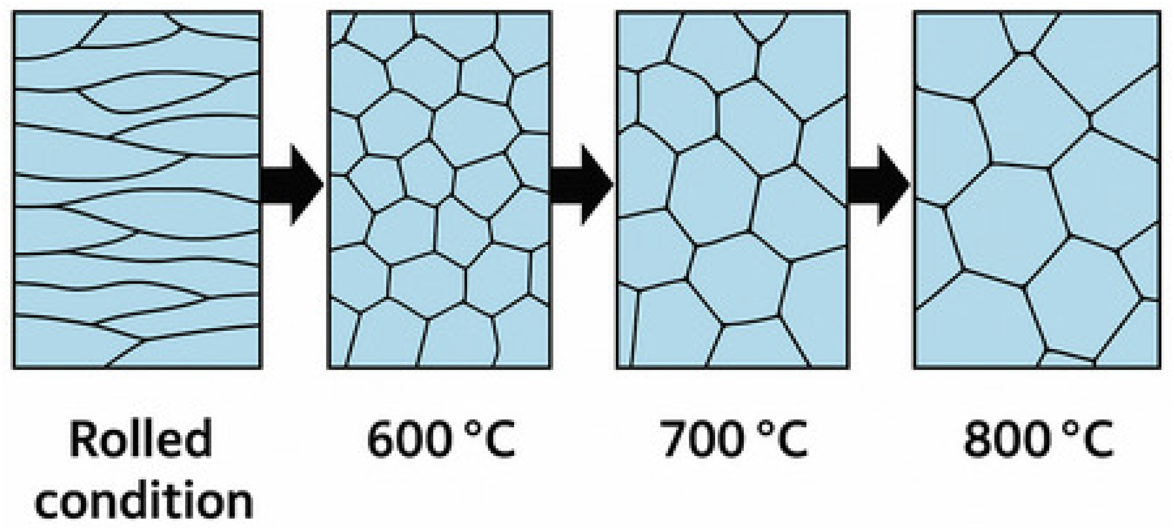
Large coil dimensions and a tightly wound geometry often lead to significant thermal gradients between the outer and inner layers. If the inner coil does not reach the target temperature, microstructural inhomogeneity may occur, affecting properties and downstream formability. Figure 3 illustrates microstructure evolution during annealing at different temperatures [46,47,48,49,50]. Accurate prediction of the inner coil temperature is therefore critical for process optimization and quality control.
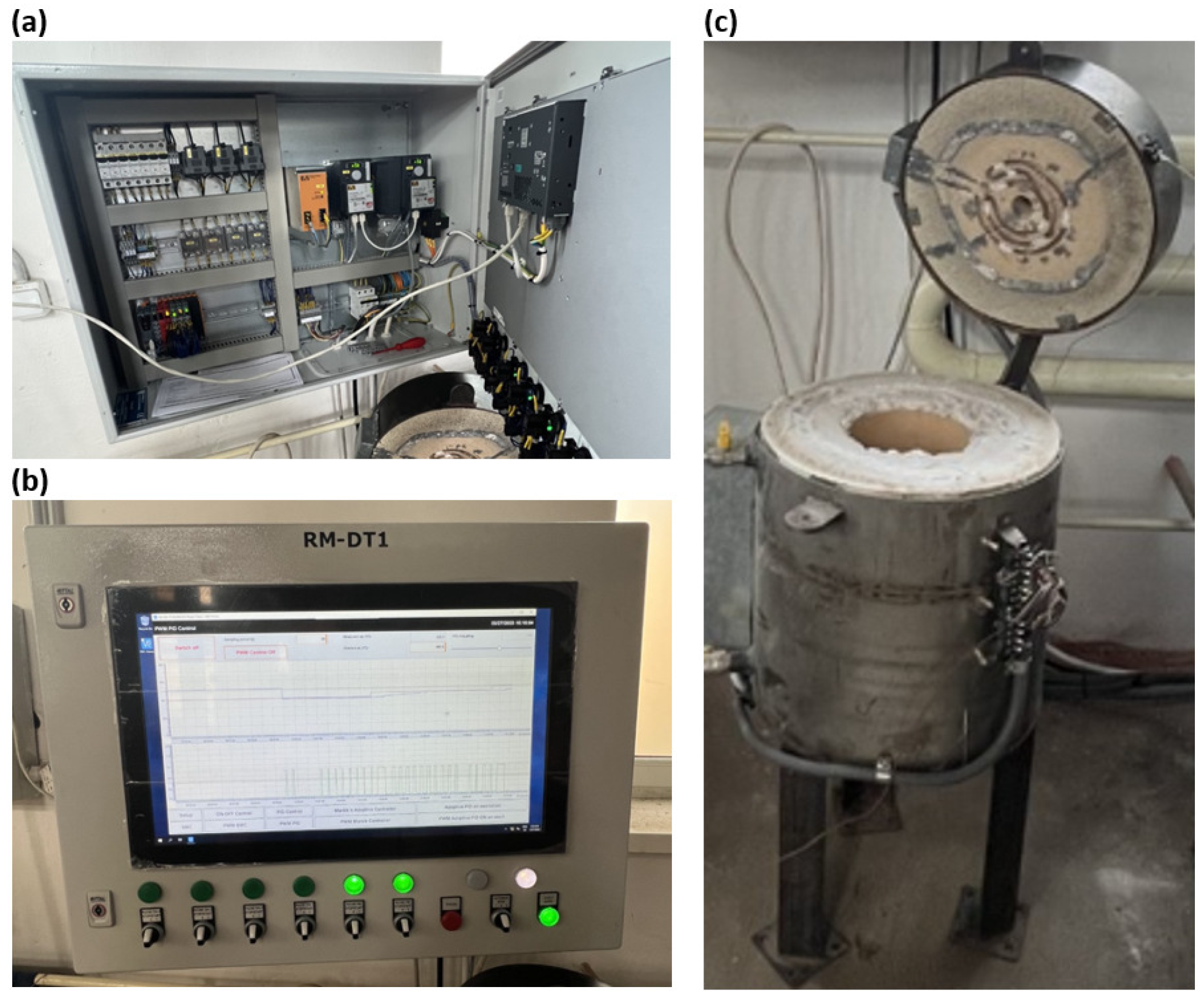
In this study, data from operational measurement (real annealing cycles) have also been used. In the industrial setup, thermocouples were manually placed on the surface and inside the steel coils before the start of the annealing cycle. The coils were loaded into the bell-type furnace and subjected to the standard heating program used in production. Temperature data were collected throughout the process using the PLC, serial link (RS232), and the PC for data recording. The resulting datasets reflect real operational conditions and were used for model proposal and validation. Figure 4 depicts the experimental measurement system used for annealing tests. The setup includes K-type thermocouples, a PLC unit (B&R 2005), and a PC with OPC-based communication. The authors of this study have developed custom software for recording and visualizing temperature profiles on a lab scale and in operation [51]. For verification of model-based (soft-sensor) temperature estimation, control measurements were also conducted by placing thermocouples between the coil windings.
This overview of the annealing process and measurement setup provides the context for developing and validating the individual physics-based and machine learning models whose predictive performance is compared in the following sections.

4. Materials and Methods

4.1. Experimental Annealing Furnace

A series of experiments was conducted using an electric-heated laboratory bell furnace, adapted for testing temperature modeling techniques (see Figure 5). For validation purposes, a physical model of a steel coil was placed inside the furnace, where electric spirals provided heating. The model coil was instrumented with K-type thermocouples to measure temperatures at three critical locations: directly on the heating spirals (i.e., control temperatures), on the surface of the coil (i.e., surface temperatures), and within the coil (i.e., internal temperatures).
The actual internal temperatures, along with surface temperatures, were measured during annealing using thermocouples. The internal temperatures were obtained from thermocouples inserted into the inner windings at various positions within the selected steel coils. These measurements were recorded continuously throughout the heating, holding, and cooling phases of the annealing cycle, providing accurate reference data for model development and validation.
The experimental setup enabled the investigation of soft-sensing techniques for internal coil temperature estimation under realistic annealing conditions. Due to the technical limitations of the furnace, continuous control of electric power (400 VAC) was not possible. Therefore, heating was controlled using a digital signal (24 VDC) to switch the spirals on and off, maintaining a desired power level. On the side of the furnace, there are inlet valves for supplying nitrogen to prevent the rapid oxidation of the charge. A physical model of a steel coil was used as the charge for this laboratory furnace. The furnace has a volume of 0.00502 m3, the height of the furnace space is 0.25 m, and the diameter of the furnace space is 0.16 m.
The experimental procedure consisted of placing the coiled steel sheet into the laboratory furnace and initiating a controlled annealing cycle. Thermocouples were inserted into selected inner windings and attached to surface locations to capture temperature profiles during the process. The annealing cycle included a heating ramp, a holding period at the target temperature, and natural cooling, all of which were recorded by a self-made data acquisition system. Each annealing experiment followed the same procedure to ensure consistency for model proposal and validation.
The control system was implemented on a B&R PLC platform (see Figure 6), as described in [11,52]. It utilized a combination of pulse-width modulation (PWM), classical PID control, ON–OFF regulation, and sliding mode control (SMC) [52]. The monitoring system enabled heating control based on either measured surface temperatures or model-estimated inner coil temperatures via a soft sensor.

4.2. Modeling Methods for Modeling Internal Temperatures

This section presents two distinct approaches suitable for estimating the internal temperature of steel coils during the annealing process. The first approach utilizes the theory of transient (non-stationary) heat conduction, while the second applies support vector regression (SVR), a machine learning technique. The former follows a physics-based analytical formulation, whereas the latter operates as a data-driven black-box model.

4.2.1. Modeling Basedd on Finite Difference Method

The transient heat conduction within the steel coil was modeled using the Fourier–Kirchhoff equation in cylindrical coordinates ( r , z ) under the assumption of rotational symmetry (no dependence on the azimuthal coordinate θ ). This formulation better represents the actual geometry of the coil, where temperature gradients predominantly occur in the radial and axial directions [53,54]:
T τ = α 2 T r 2 + 1 r T r + 2 T z 2 ,
where T is the temperature ( K ) , α = λ ρ c p is the thermal diffusivity ( m 2 s 1 ) , λ is the thermal conductivity ( W m 1 K 1 ) , ρ is the density ( kg m 3 ) , and c p is the specific heat capacity ( J kg 1 K 1 ) , and τ is the time ( s ) .
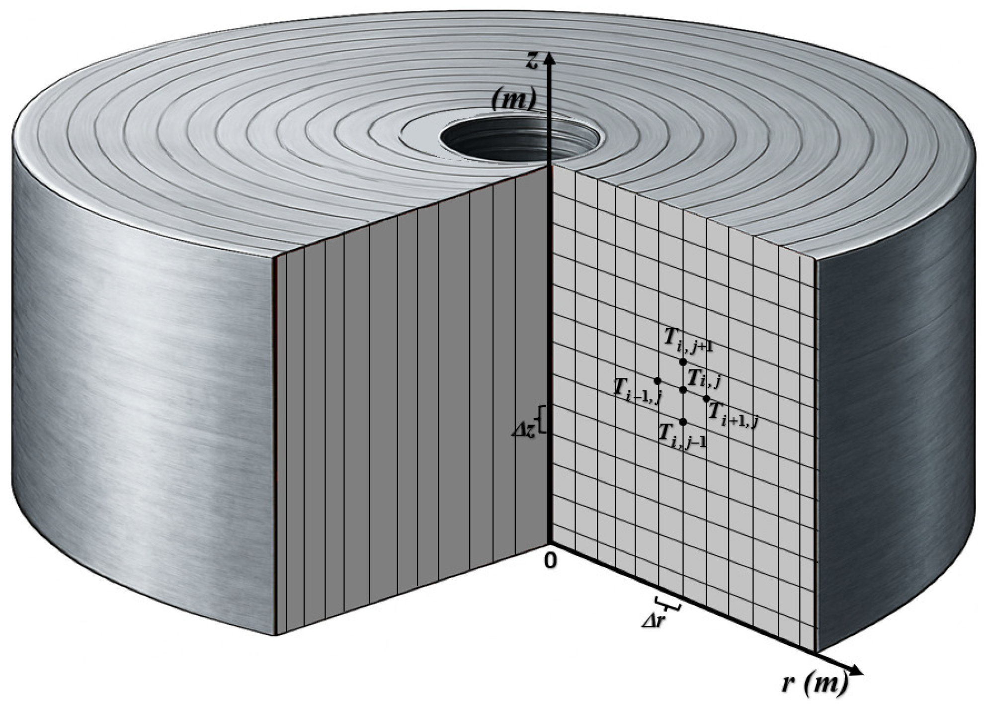
The computational domain was defined as a two-dimensional axisymmetric cross-section of the coil. The coil was discretized into a uniform grid with Δ r and Δ z spacing. The explicit finite difference scheme was applied for time integration. The discrete form of Equation (1) at node ( i , j ) and time step n is [54,55]:
T i , j n + 1 = T i , j n + F o r T i + 1 , j n 2 T i , j n + T i 1 , j n + Δ r 2 r i T i + 1 , j n T i 1 , j n + F o z T i , j + 1 n 2 T i , j n + T i , j 1 n ,
where
F o r = α Δ τ Δ r 2 , F o z = α Δ τ Δ z 2 ,
and r i is the radial position of the i-th grid point. Parameter Δ r is the radial grid spacing (m), Δ z represents axial grid spacing (m), and Δ τ is the time step (s).
The scheme stability is governed by the following condition:
F o r + F o z 1 2 .
Figure 7 illustrates the computational mesh for the axisymmetric finite difference model of the steel coil. The r-axis represents the radial direction from the coil’s center, and the z-axis corresponds to the coil’s vertical symmetry axis. Temperature values T i , j are computed at each internal grid node, while T i ± 1 , j and T i , j ± 1 denote the four neighboring nodes used in the discretized heat conduction equation.
Boundary conditions were derived from experimental measurements and the physical characteristics of the annealing process. Table 1 summarizes the applied boundary conditions and the thermophysical properties used in the simulation.
Typical ranges are based on literature values for low-carbon steels during heating [56]. For the numerical simulations in this study, constant values within these ranges were adopted: λ = 31.322 W m 1 K 1 , ρ = 7800 kg m 3 , c p = 502.4 J kg 1 K 1 , and α = 8.01 × 10 6 m 2 s 1 . These values were calibrated against laboratory and industrial annealing measurements to ensure that the FDM model realistically represents the thermal behavior of the coil.
The model allows for flexible incorporation of experimentally measured surface temperatures as time-dependent Dirichlet boundary conditions. This approach ensures that the simulated internal temperature evolution reflects realistic heating conditions during the annealing process.
The core of the FDM-based simulation lies in the discretization of the transient heat conduction Equation (2) in axisymmetric cylindrical coordinates ( r , z ) .
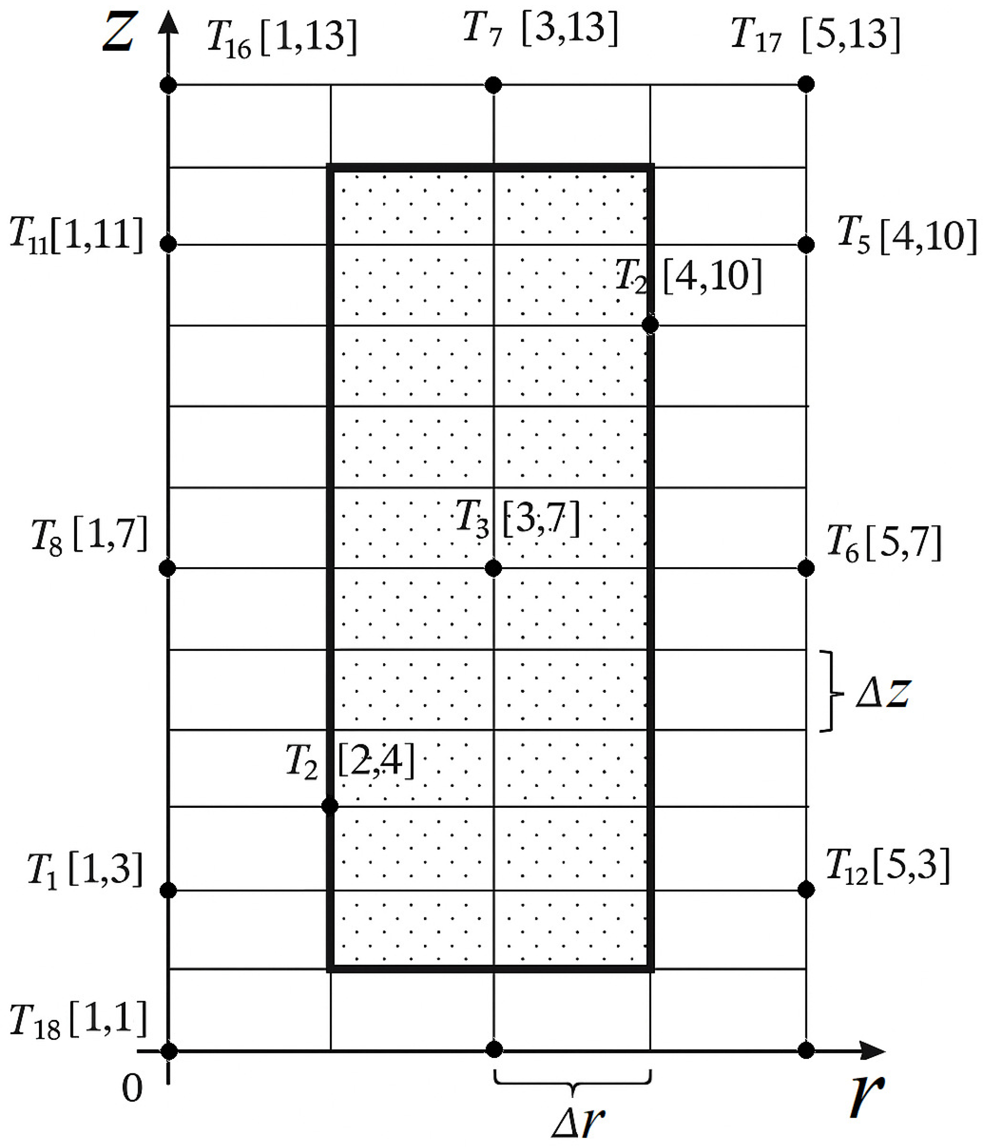
The domain was represented as a 2D axisymmetric grid spanning r [ 0 , R ] and z [ 0 , H ] . The grid resolution was defined by the number of nodes M in the radial direction and N in the axial direction, with uniform spacings Δ r and Δ z . The time step Δ τ was selected to satisfy the stability criterion F o r + F o z 0.5 , where F o r = α Δ τ / Δ r 2 and F o z = α Δ τ / Δ z 2 . The physical model of the steel-sheet coil had the following setup ( Δ r = 0.00375 m, Δ z = 0.00790 m, M = 5, N = 13 ) [3].
Figure 8 shows the placement of thermocouples mapped onto the r-z cross-section of the coil. At the coil centerline ( r = 0 ), a symmetry condition T r = 0 was applied. At the radial outer boundary ( r = R ), time-varying Dirichlet boundary conditions were assigned based on measured surface temperatures. The axial ends ( z = 0 and z = H ) were treated as adiabatic or as Dirichlet boundaries when measurements were available. Missing boundary measurements were interpolated linearly from neighboring points.
The algorithm computed the temperature at each interior grid node iteratively in time, while boundary nodes were fixed at their prescribed values for each time step. All computed temperature fields were stored for post-processing and analysis.
To improve accuracy, an adaptive calibration procedure adjusted α , λ , and c to minimize the mean absolute deviation between simulated and measured temperatures at selected control points inside the coil:
J = 1 N t N p k = 1 N t j = 1 N p T sim , j k T mer , j k ,
where N t is the number of time steps, N p is the number of control points, T sim , j k is the simulated temperature, and T mer , j k is the measured temperature at point j and time k. The optimization combined gradient-based and dynamic programming methods [51].
Recently, Durdán et al. [57] applied a similar axisymmetric FDM approach to estimate thermal diffusivity α during annealing using deterministic nonlinear optimization, achieving significant error reduction when validated against experimental data from a bell-type furnace.

4.2.2. Modeling Based on Machine Learning (ML)

Support Vector Regression (SVR)
Support vector regression (SVR) is a powerful machine learning (ML) technique used for modeling nonlinear regression problems. Its theoretical foundation is based on the concept of mapping the original input space into a higher-dimensional feature space, where a linear regression function is constructed. This approach enables the approximation of complex nonlinear dependencies while maintaining good generalization performance, especially when the number of training samples is limited [58,59].
Input data (i.e., the coil’s surface temperatures as observations) are represented by the vector x = ( x 1 , x 2 , , x l ) , where l denotes the size of the sample. Given a training dataset consisting of input–output pairs ( x i , y i ) , i = 1 , , l , SVR seeks a function f ^ ( x ) that deviates from the true targets by no more than a margin ε for each training sample while remaining as flat as possible. In our case, this function finds the target internal temperature in the annealed coil based on input observations (surface temperatures of the coil). The regression function takes the following form:
y T = f ^ ( x ) = i = 1 l α i α i * K x i , x + b ,
where α i and α i * are Lagrange multipliers, b is a bias term, and K is a symmetric, positive kernel matrix, such as linear, Gaussian, or polynomial, generated directly by a kernel function, i.e., K = ( k ( x i , x j ) ) i , j = 1 l . Only a subset of the training samples with nonzero α i or α i * , called support vectors, contribute to the final prediction [60,61].
The optimization task is to minimize the following objective:
L ( α ) = 1 2 i = 1 l j = 1 l α i α i * α j α j * K ( x i , x j ) + ε i = 1 l α i + α i * i = 1 l y i α i * α i .
To determine the optimal values of α , the optimization problem involves minimizing the Lagrange function [62,63] while guaranteeing compliance with the Karush–Kuhn–Tucker (KKT) complementary conditions [58,64].
In this study, SVR was used to estimate internal coil temperatures during annealing based on surface temperature measurements. To assess generalization, SVR models were tested on datasets other than the training dataset. The SVR implementation in MATLAB was used with a linear, Gaussian, and polynomial kernel [62,63]:
  • Linear kernel:
    k ( x i , x j ) = x i T x j .
  • Gaussian kernel:
    k ( x i , x j ) = e γ | | x i x j | | 2 ,
    where γ is the kernel width parameter.
  • Polynomial kernel:
    k ( x i , x j ) = ( γ ( x i T x j + 1 ) ) d ,
    where d is an integer.
Sequential minimal optimization (SMO) was employed to solve the underlying quadratic programming problem efficiently. The advantage of SVR in this application lies in its ability to handle nonlinear relationships between surface and internal temperatures while relying on a limited number of support vectors, making the model computationally efficient and robust to overfitting. The use of support vector regression (SVR) in modeling annealing operations is reported in [3].
The SVR model was trained on real measured data (laboratory and operational) collected during experimental annealing cycles, with input–output pairs formed by surface and internal temperatures obtained from thermocouples. This approach allows estimation of inner temperatures using only surface measurements in practical applications where internal sensors are not feasible.
For SVR modeling, the MATLAB Statistics and Machine Learning toolbox [62,63] was utilized.
Feed-Forward Neural Networks
Another approach being investigated for modeling internal coil temperatures is based on a neural network (NN). Feed-forward neural networks (FNNs) represent a class of supervised learning models capable of approximating nonlinear functions through layered processing of input data. In this work, a classical back-propagation neural network (BPNN) was used to predict the internal temperature of a steel coil during annealing, based on surface temperature measurements. The network structure consists of an input layer, two hidden layers with N neurons in the first hidden layer, and a single output neuron. The number of neurons in the hidden layer was set based on the recommendation in [65]. Similar applications of FNN to the annealing process can be found in [28].
In neural network training, the goal is to compute the weights and thresholds that relate the input vector of activities x to the expected output vector y ^ [65].
Each neuron in the hidden layer computes a weighted sum of its inputs and applies a nonlinear activation function to the result. The output of the j-th hidden neuron is calculated as follows:
L j = f i = 1 n w i j x i θ j , j = 1 , 2 , , N ,
where x i are the input features (surface temperatures), w i j are the connection weights, θ j is the bias term, and f ( · ) is the transfer function. In our experiments, the log-sigmoid activation function was used.
The output neuron aggregates the contributions from hidden neurons and subtracts a bias:
y T = j = 1 N L j w j a ,
where w j are the output layer weights, and a is the output neuron bias [66].
Training was performed using the gradient descent method with momentum and adaptive learning rate. The network minimizes the mean squared error between predicted and true internal temperatures:
E = 1 2 i = 1 M ( y i y ^ i ) 2 ,
where M is the number of training samples. The learning parameters (i.e., learning rate, momentum, and number of epochs) were experimentally tuned to ensure stability and convergence.
The number of input features (i.e., measured surface temperatures) varied between experiments. In the case of laboratory data, 15 inputs were used, resulting in a neural network architecture of 15-31-1-1. For the two industrial datasets, the number of input features was 5 and 4, leading to architectures of 5-11-1-1 and 4-9-1-1, respectively. These configurations were derived from the commonly used heuristic 2 d + 1 for the number of neurons in the hidden layer. Despite the differences in structure, all neural networks were trained using the same algorithm and hyperparameters: a log-sigmoid activation function, gradient descent with momentum 0.9, an adaptive learning rate ( 10 9 ), and a maximum of 1000 epochs. The output of each network was a single neuron representing the predicted internal temperature.
Multivariate Adaptive Regression Splines (MARS)
Multivariate adaptive regression splines (MARS) is a flexible, non-parametric regression method introduced by Friedman [67], capable of modeling nonlinear relationships and variable interactions without requiring a priori functional forms. MARS has been effectively applied in various fields, including recent studies on temperature prediction in steelmaking [68]. However, the MARS application for predicting temperatures in the annealing process has not yet been published.
The core idea of MARS is to approximate the target variable y T as a sum of basis functions (BFs), which are constructed from piecewise-linear or piecewise-cubic splines. The model takes the following form:
y T = f ^ ( x ) + ε = c 0 + m = 1 M c m B m ( x ) + ε ,
where y T is the predicted inner temperature in the coil, x denotes the input vector (e.g., surface temperatures), c 0 is the intercept, M indicates the total number of basis functions (BFs) in the model (i.e., spline functions), c m are coefficients of basis functions B m ( x ) , and ε is the error term.
To construct BFs, MARS introduces knots at observed data points, splitting the input domain and generating reflected pairs for each variable. Piecewise-linear splines typically use the hinge function:
max ( 0 , x t ) = x t , if x t 0 , otherwise ,
where t is the knot.
The cubic basis function, utilized in some implementations [69], can be written in the following form:
C ( x | s = + 1 , t , t , t + ) = 0 , x t α + ( x t ) 2 + β + ( x t ) 3 , t < x < t + x t , x t + ,
with the following coefficients:
α + = 2 t + 3 t + t ( t + t ) 2 , β + = t + + 2 t t ( t + t ) 3 .
A mirrored form C ( x | s = 1 , t , t , t + ) is defined analogously:
C ( x | s = 1 , t , t , t + ) = t x , x t α ( x t + ) 2 + β ( x t + ) 3 , t < x < t + 0 , x t + ,
with
α = t + + 3 t 2 t ( t t + ) 2 , β = t + 2 t + t ( t t ) 3 .
The MARS algorithm proceeds in two stages: forward selection, where an overfitted model is built by adding BFs, and backward pruning, where unimportant terms are removed. The final model strikes a balance between accuracy and generalizability. In our study, the implementation by Jekabsons [70] was used, testing both linear and cubic variants. A rule of thumb constrained the number of basis functions: min ( 200 , max ( 20 , 2 d ) ) + 1 , where d is the number of predictors.
Although all MARS models were initialized using the same configuration parameters, the final number of basis functions (BFs) selected after pruning varied depending on the dataset. Specifically, the model trained on laboratory data with 15 input features resulted in 8 final BFs. For the two industrial datasets, which used 5 and 4 input variables, respectively, the final models retained 19 and 18 BFs. These differences reflect the adaptive nature of the MARS algorithm, which adjusts model complexity based on the data dimensionality and structure.
k-Nearest Neighbors Regression
The k-nearest neighbors (k-NN) algorithm is a non-parametric approach, initially introduced by Fix and Hodges [71] and later refined for broader machine learning applications [72,73,74]. In this work, k-NN regression was utilized as an alternative strategy for predicting the internal temperatures of annealed steel coils from their surface temperature measurements.
The method estimates the output y T for an unseen input x by averaging the values of its k nearest neighbors in the training data. In the basic variant with uniform weighting, the estimate is computed as follows:
y T = f ^ ( x ) = 1 k i N k ( x ) y i ,
where N k ( x ) denotes the index set of the k closest training samples to x under a chosen metric.
The distance metric used in our implementation was Euclidean distance, the most common choice in practice. Optionally, distance-based weighting can be applied, where closer neighbors contribute more to the following prediction:
y T = f ^ ( x ) = i N k ( x ) w i y i i N k ( x ) w i , w i = 1 d i ,
where d i is the distance between x and the i-th neighbor.
Our implementation was based on the open-source k-NN regressor by Ferreira [75], and used k = 5 with uniform weights. The training phase involved storing the whole training dataset ( x i , y i ) without model fitting, and predictions were made by distance-based lookups at test time. This lazy learning property makes the k-NN conceptually simple yet powerful for local approximation.
Random Forests
Random forests (RFs) are robust ensemble learning algorithms suitable for both classification and regression, initially introduced by Ho [76] and later extended by Breiman [77]. The technique builds multiple decision trees on bootstrapped subsets of the data and aggregates their outputs. In regression tasks, the final prediction is the average of the outputs from all individual trees [73,74].
The RF algorithm operates by randomly selecting training samples with replacement and fitting unpruned decision trees to each subset. If the input training dataset consists of n samples with input vectors x = { x 1 , x 2 , , x n } and corresponding temperature responses y = { y 1 , y 2 , , y n } , then the model constructs B trees via bootstrap aggregation (bagging) as follows:
  • For each b = 1 , , B ,
    generate x b and y b by sampling n instances with a replacement from the original dataset;
    train a regression tree f b on this sample.
Once the ensemble is trained, the prediction for a new input x is provided by the following:
y T = f ^ ( x ) = 1 B b = 1 B f b ( x ) ,
where y T denotes the predicted internal temperature, and f b is the b-th decision tree in the forest.
In our study, we employed a generic implementation of the Random Forest (RF) algorithm, as proposed by Banerjee [78], adapted for regression tasks in MATLAB. The number of trees was set to B = 5000 , which provides a balance between prediction accuracy and computational efficiency. Euclidean distance was implicitly used during tree construction to split nodes based on input features. The script utilized for training and prediction ensures that each tree is built independently on randomized subsets of surface temperature data, allowing the ensemble to generalize well to unseen annealing cycles.
All random forest models were trained using the same configuration across all datasets, regardless of the number of input features. Each model used 5000 decision trees, trained on bootstrap samples of the input data. The splitting criterion used for node splits was the mean squared error (MSE), which is the default in the employed MATLAB R2020b implementation. No additional pruning or depth limitation was applied. This consistent setup ensured fair comparison between experiments while preserving the robustness and generalization capability of the ensemble models.
In summary, all machine learning models were developed using consistent training parameters and methodologies across experiments, while accounting for differences in the number of input features (i.e., measured surface temperatures). The laboratory dataset used 15 inputs, whereas the industrial experiments used 5 and 4 inputs, respectively. This variation naturally led to different model structures: neural networks with 15-31-1-1, 5-11-1-1, and 4-9-1-1 architectures, and MARS models with 8, 19, and 18 final basis functions. Random forest models were configured uniformly across all cases, with 5000 decision trees and MSE as the splitting criterion. These configurations ensured a fair and reproducible comparison of data-driven modeling approaches under varying measurement conditions.

4.2.3. Pros and Cons of Applied Methods

The finite difference method (FDM) is a widely used numerical technique for solving heat conduction problems by discretizing the governing partial differential equations. While FDM provides a physically grounded framework for thermal modeling, its accuracy and computational cost depend on grid resolution and boundary condition handling. Machine learning algorithms, in contrast, rely on previous successful strategies to make accurate predictions for the future. Each method has its strengths and limitations, which affect its suitability for specific modeling tasks. Below is a concise overview of the advantages and disadvantages of the investigated methods.
  • Finite Difference Method (FDM) for Heat Conduction Modeling
    Advantages: Based on first principles and physical laws; provides interpretable results; suitable for extrapolation beyond training data; does not require data-driven learning; useful for simulating spatial and temporal temperature evolution in solid materials.
    Disadvantages: Requires precise knowledge of material properties and boundary conditions; limited adaptability to unknown dynamics; sensitive to discretization errors; may become computationally intensive for fine grids or 3D simulations.
  • Support Vector Regression (SVR)
    Advantages: Strong capability for modeling nonlinear relationships; robust against overfitting and noisy inputs; exhibits low generalization errors.
    Disadvantages: Requires careful kernel selection; needs input normalization; harder to interpret.
  • Neural Networks (NN)
    Advantages: Powerful for nonlinear problems; flexible architecture; robust to noise and missing data.
    Disadvantages: Computationally expensive; sensitive to hyperparameters; prone to overfitting; difficult to interpret; requires large datasets.
  • Multivariate Adaptive Regression Splines (MARS)
    Advantages: Handles both linear and nonlinear relationships; automatically detects interactions; works with mixed data types.
    Disadvantages: Susceptible to overfitting; slower training on large datasets; complex interpretation.
  • k-Nearest Neighbors (k-NN)
    Advantages: Simple and intuitive; no training phase; non-parametric and adaptable.
    Disadvantages: Memory-intensive; prediction can be slow; sensitive to choice of k and distance metric.
  • Random Forests (RF)
    Advantages: High accuracy; handles missing data; robust to noise; suitable for both classification and regression.
    Disadvantages: Computationally demanding; potentially complex models; slower training with large datasets.

4.2.4. Evaluation of Model Performance

To assess the quality of temperature prediction models, several standard statistical metrics were employed. These indicators compare the predicted (simulated) and measured temperature values over a validation dataset. Rather than listing all commonly known formulas, we summarize the indicators used and their interpretations.
The predictive accuracy was primarily evaluated using the following:
  • The correlation coefficient ( r y Y ), which quantifies the linear association between predicted (simulated, Y) and measured values (y).
  • The coefficient of determination ( r y Y 2 ), representing the proportion of variance in the measured data explained by the model. An r y Y 2 value of 1 indicates a perfect fit.
  • The mean squared error (MSE), which reflects the average squared difference between predicted (simulated) and actual values.
  • The root mean squared error (RMSE) and its normalized form, relative RMSE (RRMSE), which measure average prediction error in absolute and relative terms.
  • The mean absolute percentage error (MAPE), a scale-independent indicator commonly used in regression tasks. Although some studies refer to the mean of relative errors as the mean relative error (MRE) and others as the mean absolute percentage error (MAPE), both metrics are mathematically equivalent when expressed as a percentage. Therefore, results reported using either term can be directly compared in terms of model prediction accuracy.
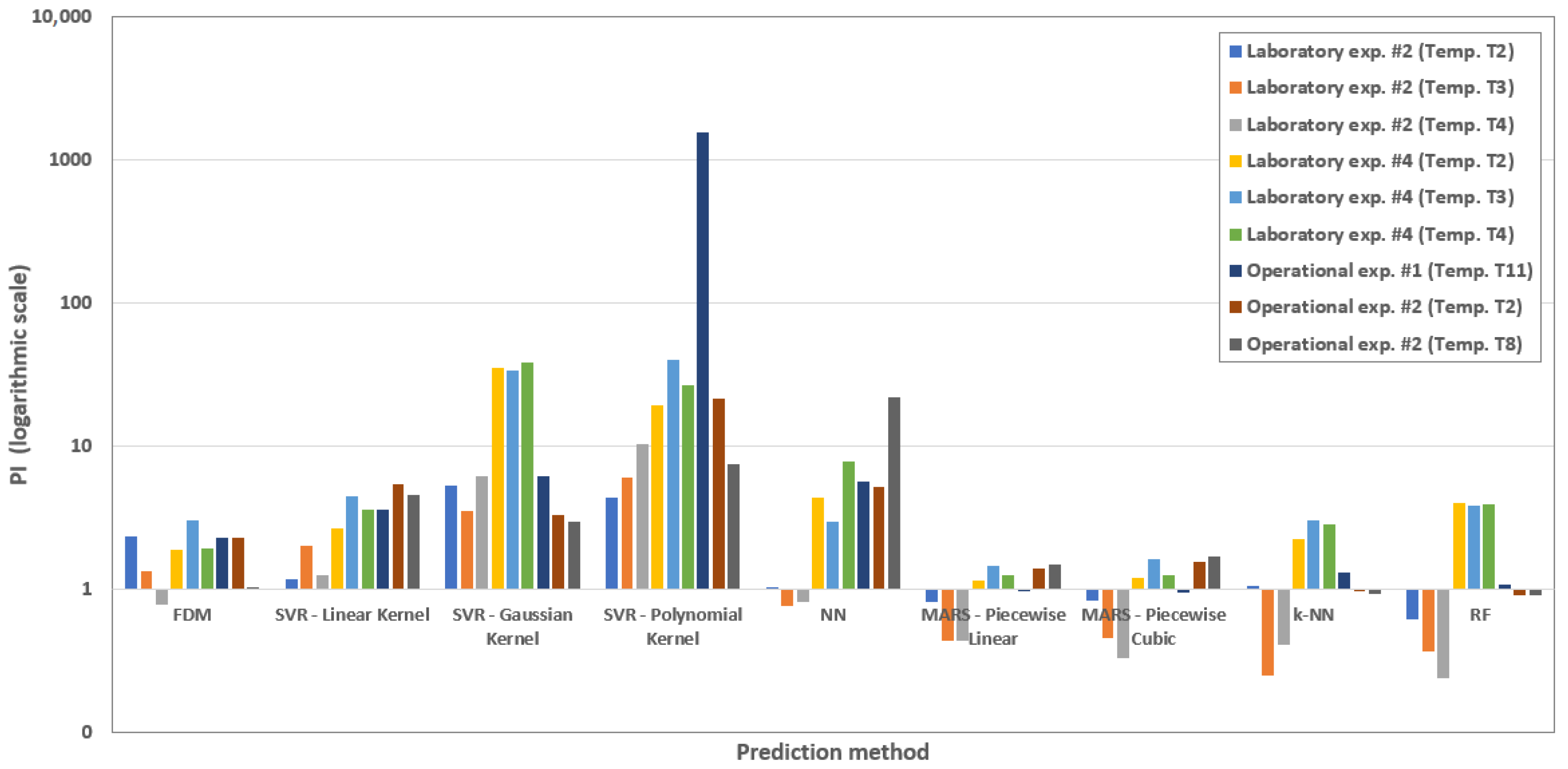
In addition to these classical metrics, a composite performance index (PI) was used, defined as the ratio of RRMSE to the correlation coefficient incremented by one (22). This index offers a robust yet straightforward comparison across models: the lower its value, the better the prediction performance [79,80].
PI = RRMSE r y Y + 1 .
Moreover, the maximum deviation between the measured temperatures and the corresponding model predictions was assessed. For each approach, the training time was also recorded to evaluate computational efficiency.

5. Results and Discussion

The following section presents and analyzes the results obtained from the application of physics-based and machine learning models to experimental data. A structured workflow was applied in the ML modeling process, as illustrated in Figure 9. Surface and internal temperatures were measured during laboratory and industrial annealing experiments. After preprocessing, the dataset was split into training and testing subsets. For all evaluated machine learning models, the training and testing datasets were derived from distinct annealing experiments. Specifically, three annealing cycles were used for training and one for testing, resulting in a 75:25 split. This approach ensured consistent and fair comparison across all predictive methods, while enabling evaluation of the models’ generalization capabilities to unseen data.

5.1. Temperature Modeling Based on Lab-Scale Measurement

In simulations of FDM, surface temperatures obtained from experimental annealing of the coils served as the primary input data for the modeling framework. A total of four laboratory electric furnace annealing experiments were performed (i.e., experiments #1–#4), using the same steel coil. The laboratory coiled sheet, serving as a physical model, exhibited a chemical composition of 0.05 wt% C, 0.3 wt% Mn, and 0.05–0.1 wt% Si.
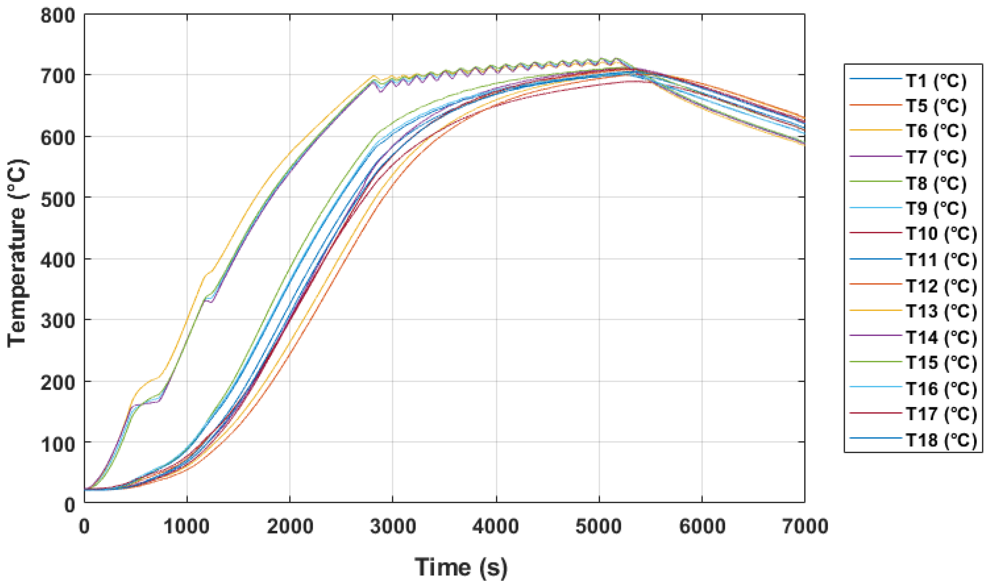
The coil was heated in a laboratory furnace, and surface temperatures were monitored and logged. The measurement setup followed the schematic representation in Figure 6. An illustration of surface temperatures captured by thermocouples during the experimental laboratory annealing is presented in Figure 10. The labels T 2 , T 3 , and T 4 indicate thermocouples placed at nodes where the recorded temperatures were compared with model predictions. The thermocouple numbering corresponds to the configuration depicted in Figure 8.
A total of 15 surface temperature observations were used to train the machine learning models (i.e., SVR, NN, MARS, k-NN, and RF) from three individual annealing experiment, i.e., x = ( x 1 , x 2 , , x l 5 ) where x 1 = T 1 , x 2 = T 5 , x 3 = T 6 , x 4 = T 7 , x 5 = T 8 , x 6 = T 9 , x 7 = T 10 , x 8 = T 11 , x 9 = T 12 , x 10 = T 13 , x 11 = T 14 , x 12 = T 15 , x 13 = T 16 , x 14 = T 17 , and x 15 = T 18 . The target variable y was always a selected internal coil temperature (i.e., T 2 , T 3 , T 4 ), which was measured by a thermocouple to train the machine models and assess their performance. The actual measured temperatures in the coil were also used to assess the performance of the FDM. The length of the training data x was 22,000 samples (for each surface temperature). Time alignment was carefully handled by trimming the beginning and end of the time series to synchronize with the available predicted temperature values, ensuring a correct comparison and evaluation of prediction accuracy. Model testing was performed on a single experiment with data x that was not used in model training. The length of the testing data was always 7000 samples. The models’ accuracy was evaluated using standard statistical metrics. In both the training and test datasets, temperatures were recorded at 1-s intervals.
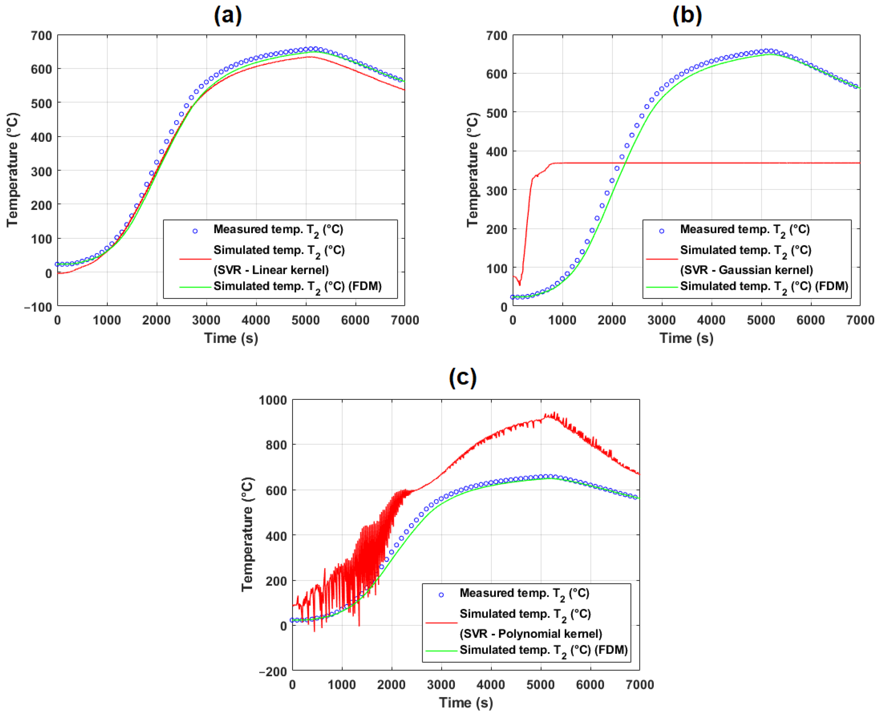
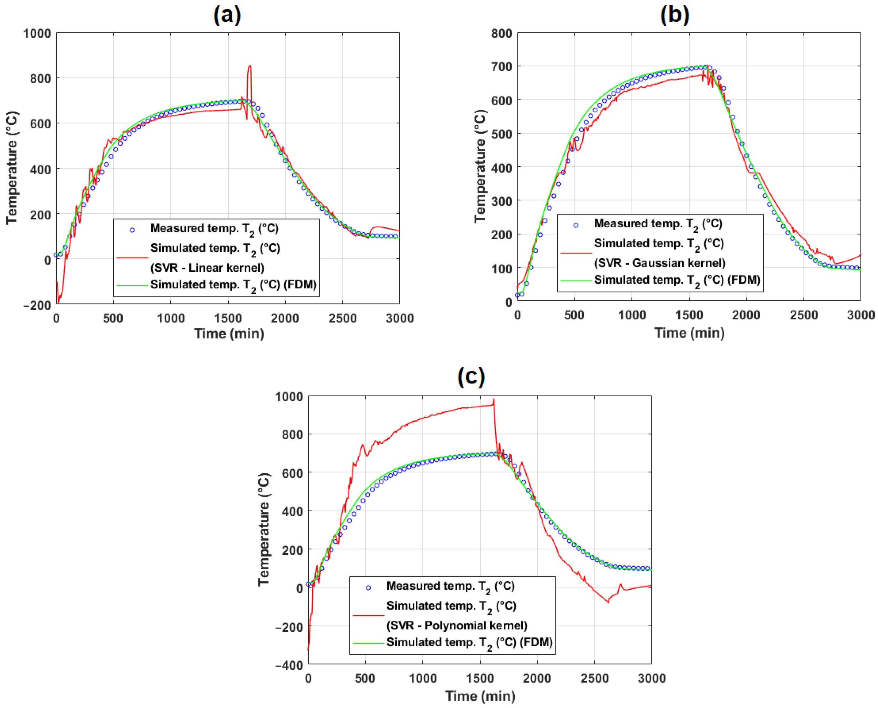
Several SVR models were created for temperature modeling, specifically for estimating inner temperatures T 2 , T 3 , and T 4 during laboratory annealing. In modeling and simulation, according to Equation (6), linear (7), Gaussian (8), and polynomial (9) kernels were used.
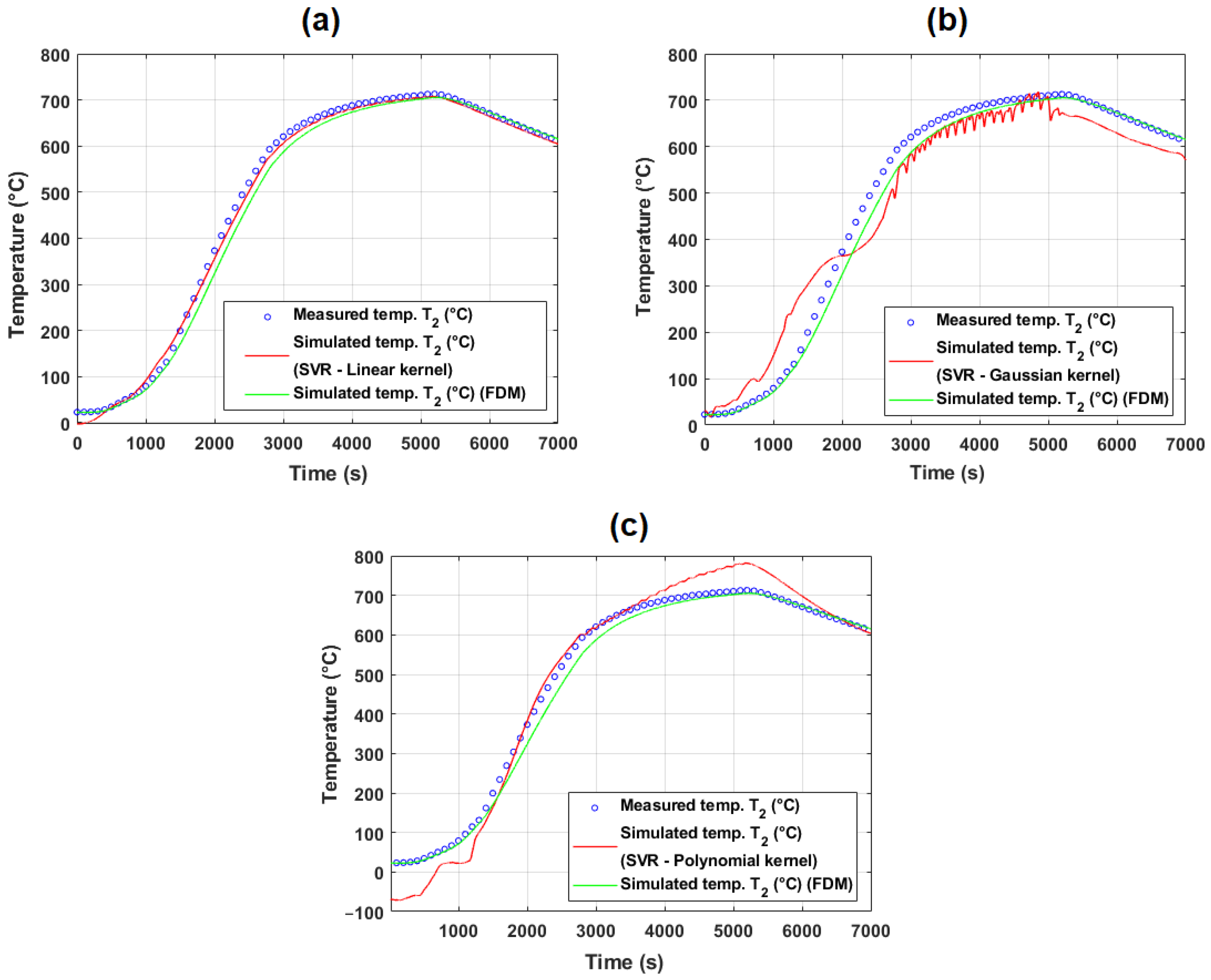
Figure 11 shows the results of simulated (predicted) inner temperature T 2 using FDM and SVR models applied on test annealing (i.e., experiment #2). For the performance assessment of the models, the plots also display the actual measured temperature T 2 obtained using a thermocouple. Similarly, Figure 12 shows results where experiment #4 was used as the annealing test.
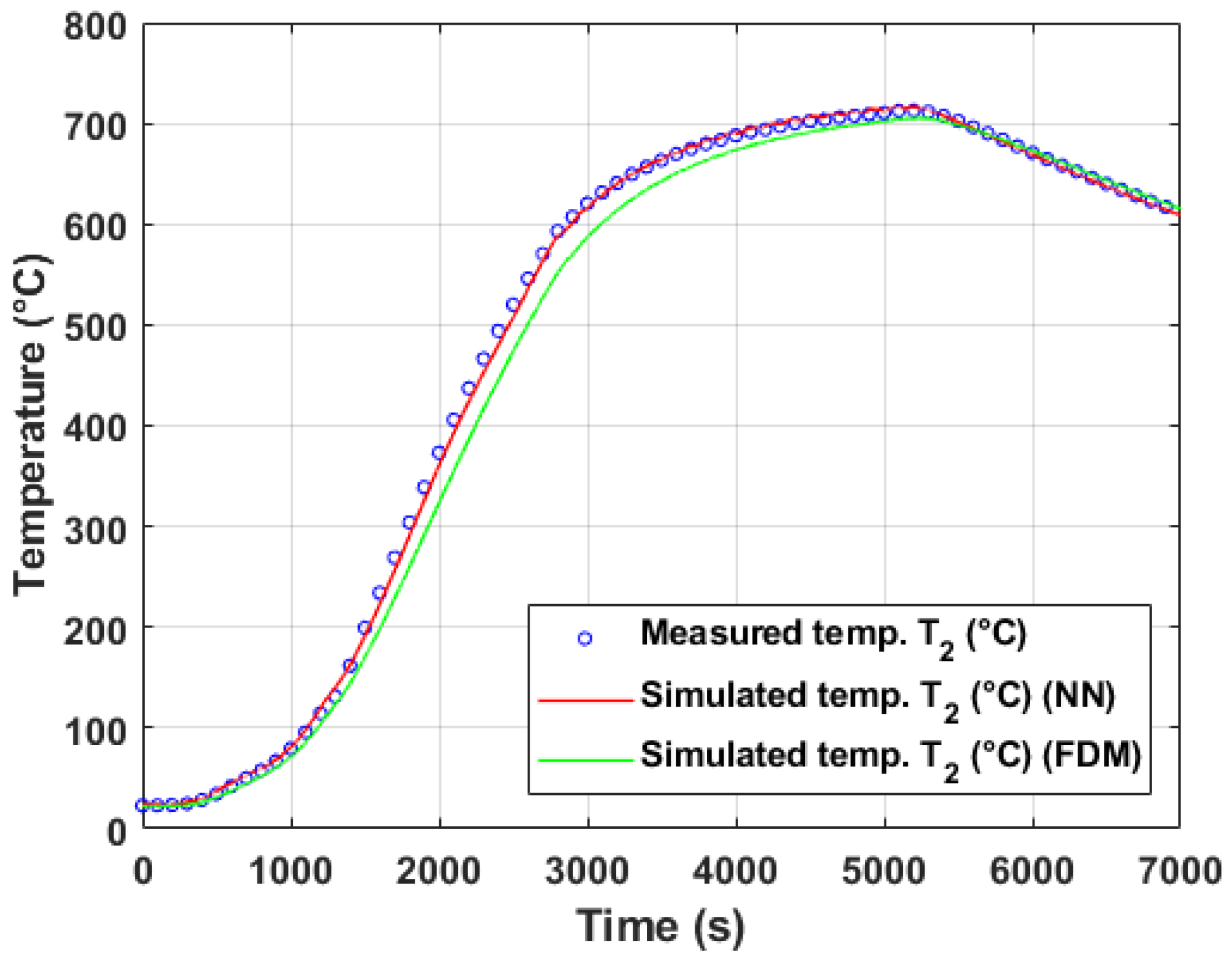
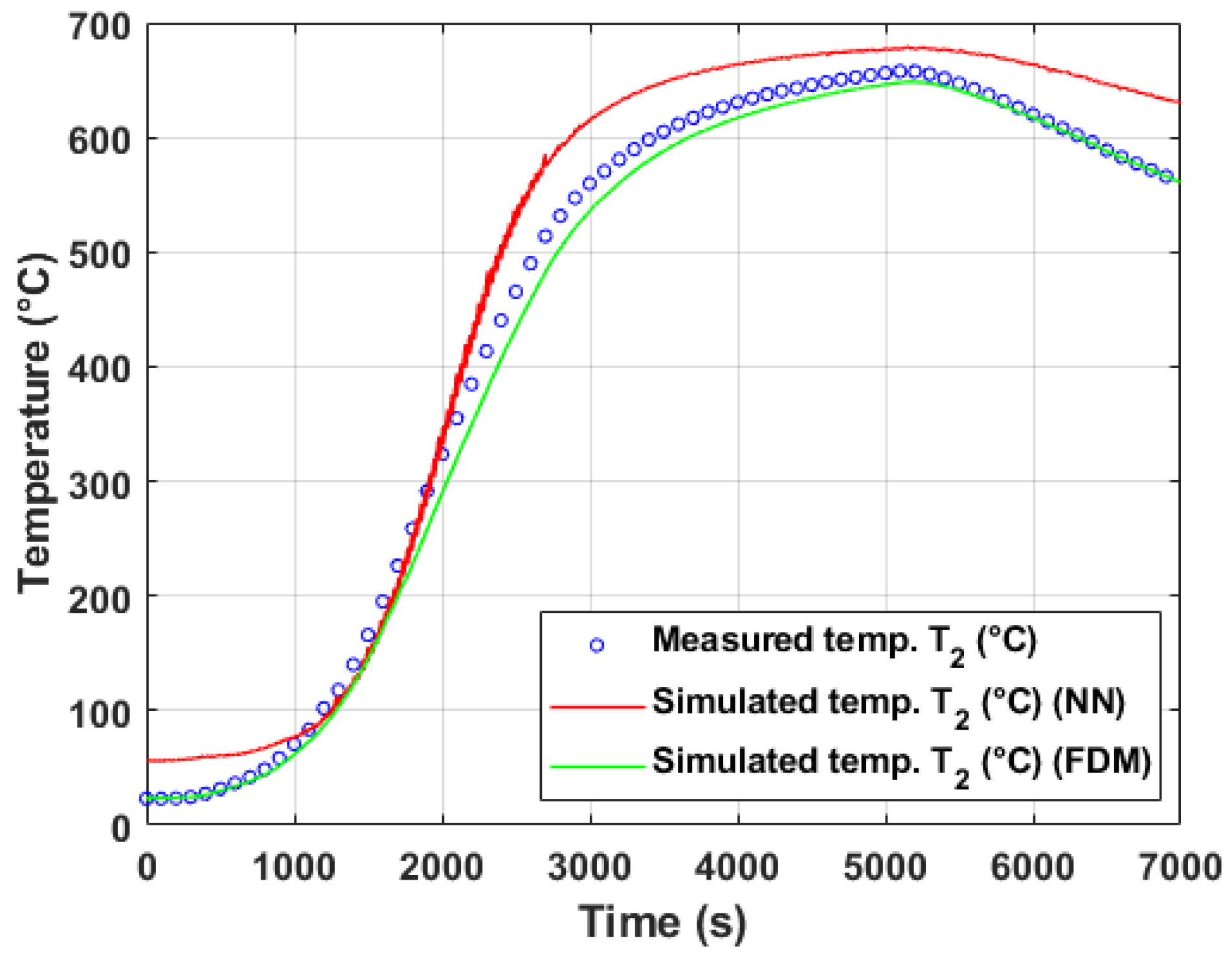
The neural network (NN) used in this study comprised two hidden layers and was trained on data from three annealing experiments, with one experiment reserved for testing. The first hidden layer contained 2 N + 1 neurons, where N = 15 input neurons, resulting in 31 neurons in total. The second hidden layer and output layer each had one neuron for predicting the target temperature. Doubling the number of hidden neurons did not improve model performance. Training was performed for up to 1000 epochs with a learning rate of 10 9 using gradient descent with adaptive learning rate and momentum (set to 0.9) to avoid local minima. The sigmoid (logistic) function was used as the activation function.
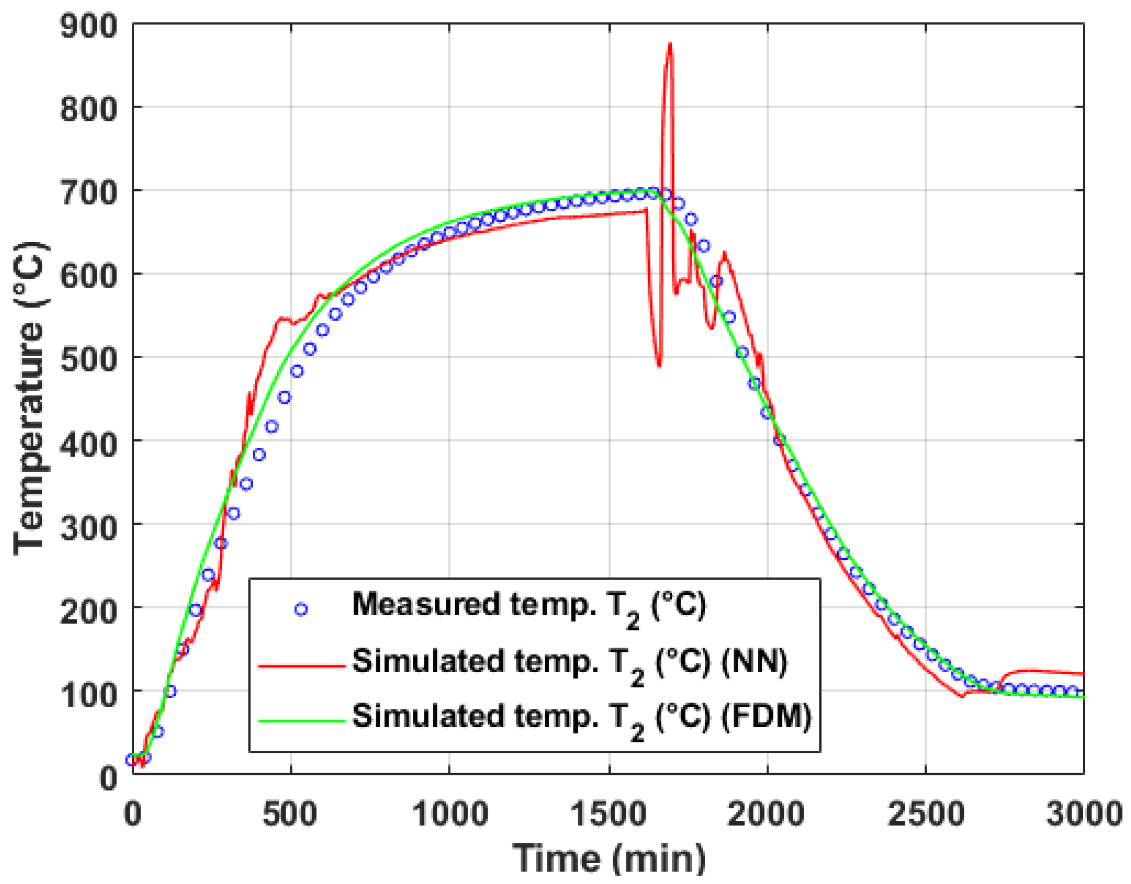
Figure 13 shows the results of the simulated (predicted) inner temperature T 2 using FDM and NN models applied on test annealing (i.e., experiment #2). For the performance assessment of the models, the plots also display the actual measured temperature T 2 obtained using a thermocouple. Similarly, Figure 14 shows the results where experiment #4 was used as the annealing test.
The MARS regression model is constructed in two stages. During the forward phase, the process starts with a model containing only the intercept term, incrementally adding pairs of reflected basis functions (BFs) to minimize training error until a predefined maximum number of BFs is reached. In the backward phase, the model is pruned by sequentially removing the least significant BFs, further reducing the error. It yields a set of candidate models of varying complexity, from which the final model is selected based on the lowest generalized cross-validation (GCV) score, subject to the maximum allowed number of BFs.
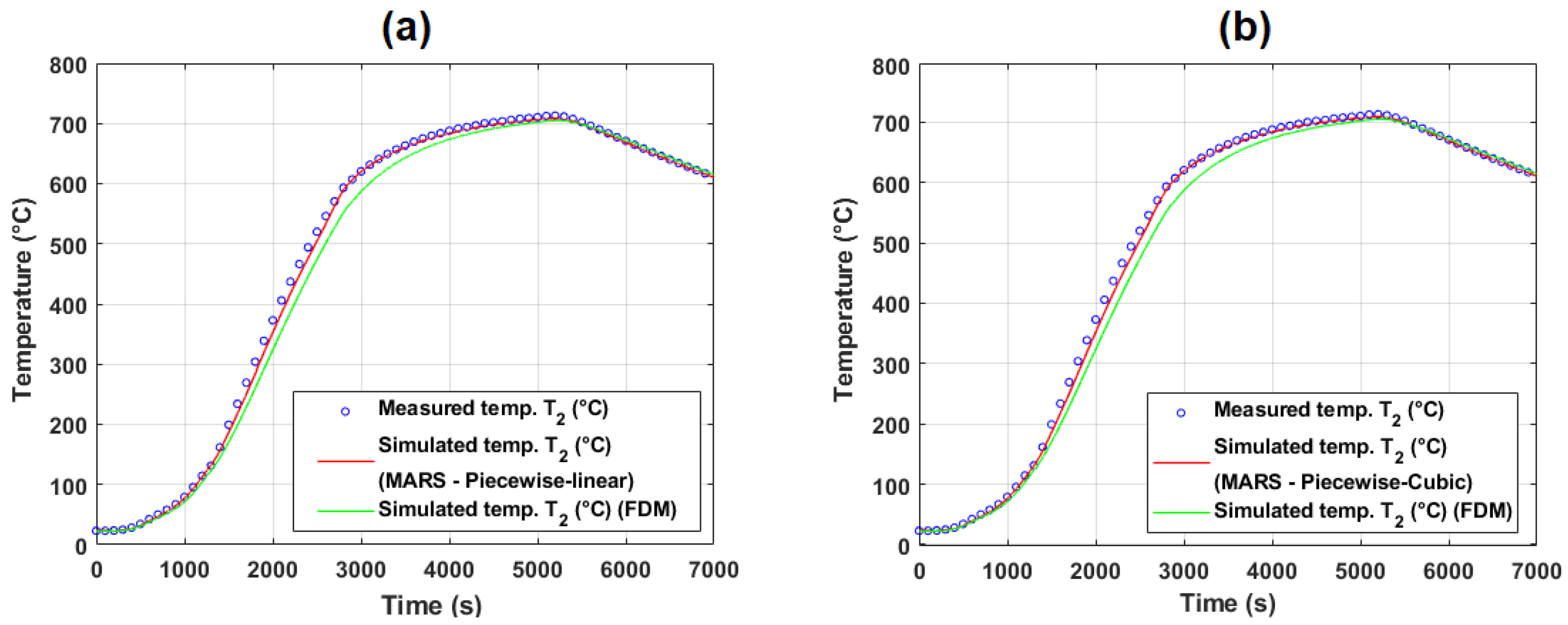
Several different variants of simulation with MARS have been performed. The created models for inner temperature prediction are portable and can be presented in the piecewise linear or cubic form. The initial number of BFs was set to 31 in all simulations. This number was reduced in the forward and backward phases of the MARS model creation. During modeling, we considered maximal interactivity between input variables without self-interactions. Since there were no smoother data, the piecewise-cubic and piecewise-linear types of modeling were analyzed to determine their prediction performance. By default, all MARS models are created as piecewise linear and transformed into piecewise cubic after the backward phase. These MARS models were created to be portable, i.e., can be presented in the form of equations and can be easily implemented in monitoring systems. The examples of mathematical equations for the selected MARS models, including all basis functions, are provided in Appendix B (see Equations (A1)–(A4)).
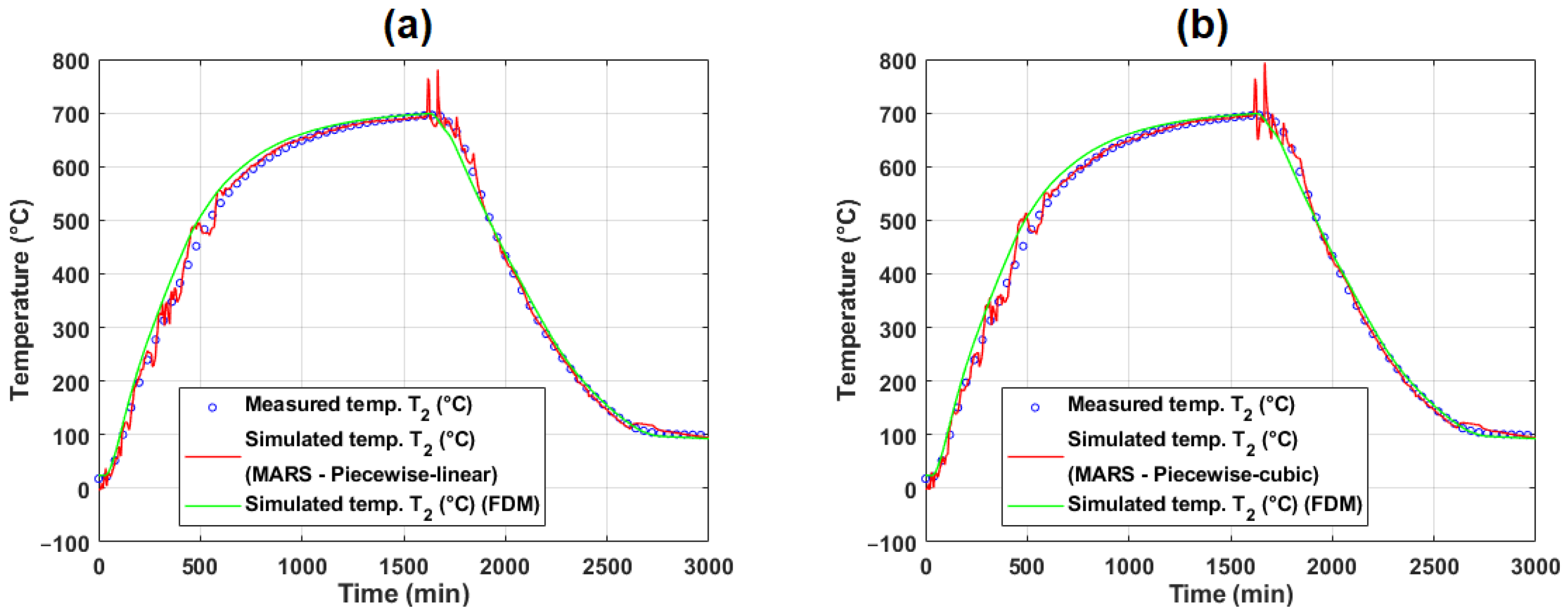
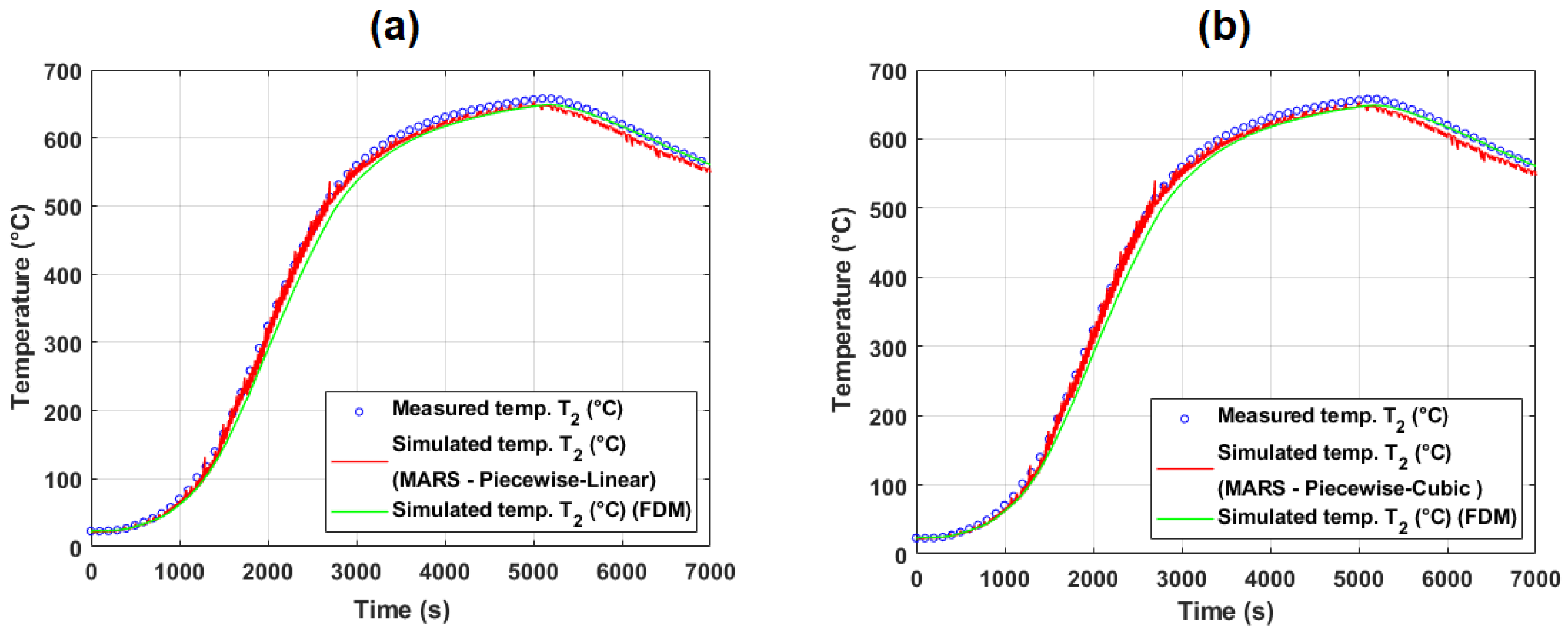
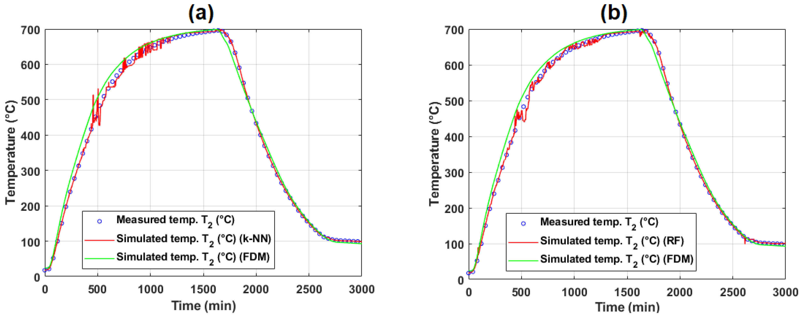
Figure 15 shows the results of the simulated (predicted) inner temperature T 2 using FDM and MARS models applied on test annealing (i.e., experiment #2). For the performance assessment of the models, the plots also display the actual measured temperature T 2 obtained using a thermocouple. Similarly, Figure 16 shows the results where experiment #4 was used as the annealing test.
The k-nearest neighbors (k-NN) regression method was the fourth method employed to predict internal temperatures within the steel coil based on surface measurements. Before model training, feature vectors were standardized using z-score normalization to ensure a uniform scale. The optimal number of neighbors, denoted as k, was set to five, based on empirical testing. It means that each prediction is derived from the five most similar observations in the training dataset. The similarity between observations was calculated using the Euclidean distance, which measures the straight-line distance in multi-dimensional feature space. To increase the influence of closer neighbors, an inverse distance weighting was applied. This assigns higher importance to nearby neighbors and reduces the impact of more distant ones, leading to smoother and more locally sensitive predictions.
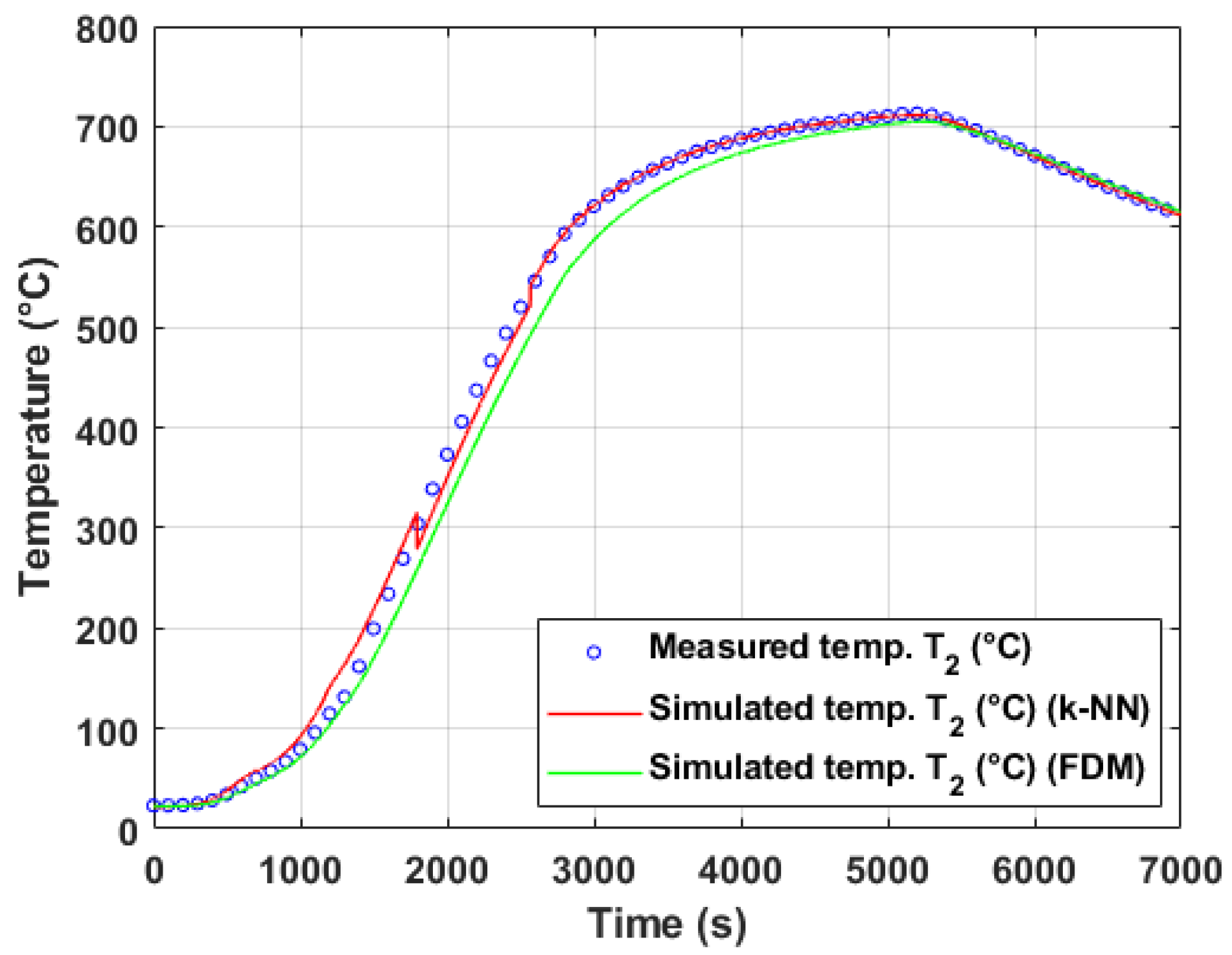
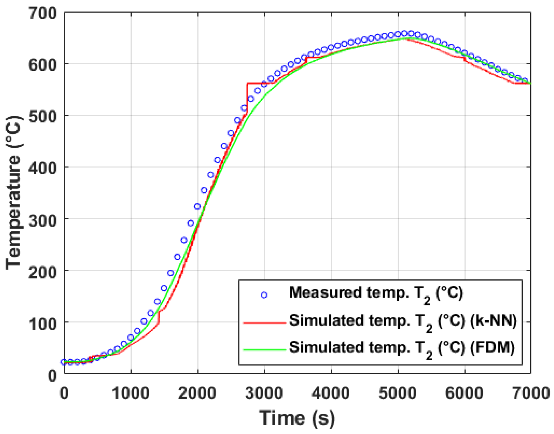
Figure 17 shows the results of the simulated (predicted) inner temperature T 2 using FDM and k-NN models applied on test annealing (i.e., experiment #2). For the performance assessment of the models, the plots also display the actual measured temperature T 2 obtained using a thermocouple. Similarly, Figure 18 shows the results where experiment #4 was used as the annealing test.
The random forest (RF) method was the last employed method to predict internal temperatures of annealed steel coils based on experimental data. The RF model utilizes a bootstrap aggregation strategy with a high number of decision tree ensembles, specifically, bags_number = 5000. This large ensemble aims to ensure model robustness and accuracy by reducing variance through resampling.
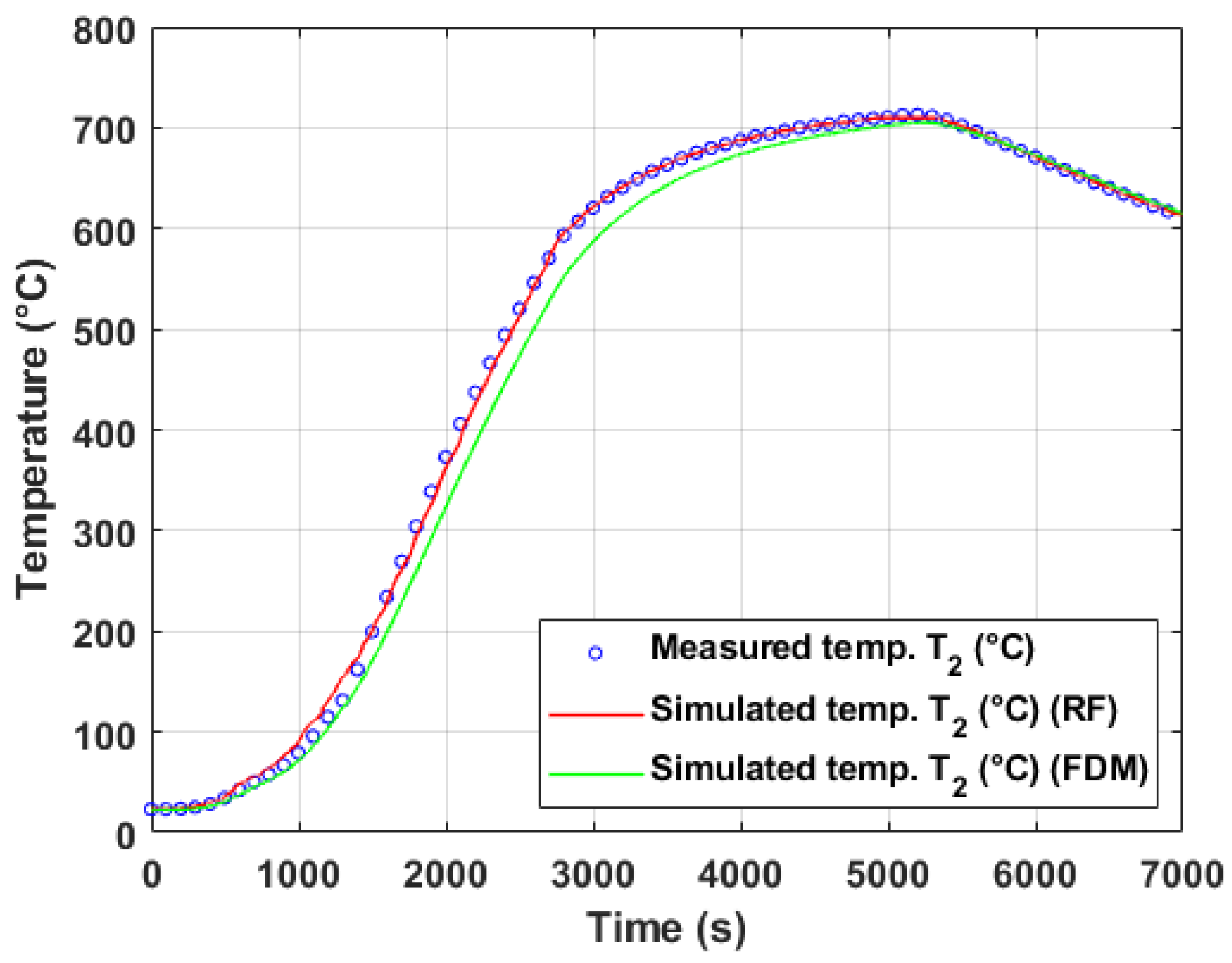
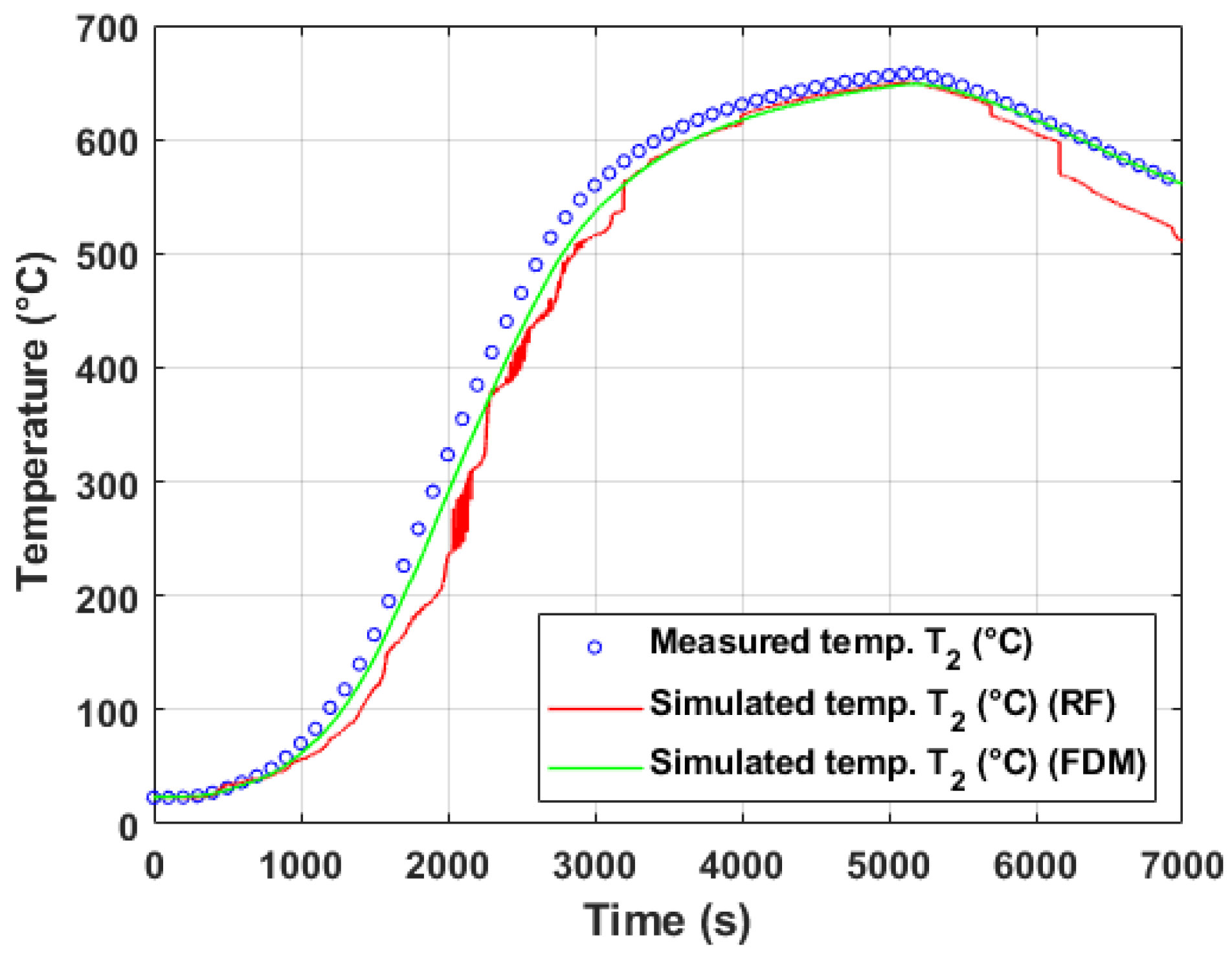
Figure 19 shows the results of the simulated (predicted) inner temperature T 2 using FDM and RF models applied on test annealing (i.e., experiment #2). For the performance assessment of the models, the plots also display the actual measured temperature T 2 obtained using a thermocouple. Similarly, Figure 20 shows the results where experiment #4 was used as the annealing test.

5.1.1. Evaluation of Model Performance on Training and Test Data (Experiment #2)

The effectiveness of the evaluated methods was assessed using multiple statistical metrics: the correlation coefficient ( r y Y ), coefficient of determination ( r y Y 2 ), mean squared error (MSE), root mean squared error (RMSE), relative RMSE (RRMSE), mean absolute percentage error (MAPE), performance index (PI), and maximum deviation between predicted and measured temperatures.
Detailed numerical results of the training phase for all models are presented in Appendix C (see Table A2). On the training dataset (experiment #2), all methods exhibited very high accuracy, with r y Y values approaching 1.0000 and r y Y 2 values close to 1.0000, indicating excellent fitting capabilities. Among the machine learning (ML) methods, the k-NN and RF achieved the lowest PI values across all three target temperatures ( T 2 , T 3 , and T 4 ), followed by the MARS models with both piecewise linear and cubic splines. SVR with polynomial kernels exhibited significantly higher errors and deviations, indicating potential overfitting issues or poor generalization for this kernel type. Training times varied significantly, with RF requiring the longest computational time due to the large number of trees in the ensemble.
In contrast, the test dataset results (Table 2) highlight the models’ generalization ability. Here, the FDM method demonstrated competitive performance, achieving high r y Y 2 values (above 0.995 for T 2 and T 3 ) and relatively low PI values. Among the ML methods, RF and MARS again performed exceptionally well, maintaining low error metrics and PI values, which demonstrates their robustness and ability to extrapolate beyond training data. Notably, SVR with polynomial kernels showed the weakest performance, characterized by large MSE, RMSE, and PI values, as well as high maximum deviations. It reinforces the earlier observation of its limited applicability for this task.
Overall, RF achieved the best predictive accuracy, closely followed by MARS, k-NN, and the neural network (NN). These findings confirm that ensemble-based and spline-based methods are well-suited for modeling and predicting internal temperatures during the annealing process. Despite the FDM being physics-based and requiring no training, it performed comparably to ML models, supporting its use in real-time simulations where computational efficiency is critical.

5.1.2. Evaluation of Model Performance on Training and Test Data (Experiment #4)

Table A3 in Appendix C summarizes the performance of individual machine learning (ML) methods during training on surface temperature data obtained from three experimental annealing cycles. The fitting accuracy of internal temperatures T 2 , T 3 , and T 4 was evaluated using several statistical indicators, including r y Y , r y Y 2 , MSE, RMSE, RRMSE, MAPE, PI, and maximum deviation. The training time for each method was also recorded. As shown in Table A3, the k-NN method and Random Forest (RF) achieved the lowest performance index (PI), indicating a nearly perfect fit on the training dataset. Multivariate Adaptive Regression Splines (MARS), in both linear and cubic variants, also provided excellent results with very low prediction errors and minimal deviations from the measured data. Support Vector Regression (SVR) with a polynomial kernel exhibited significantly higher PI values and larger deviations, indicating poorer performance in capturing the training data trend.
Table 3 presents the predictive performance of FDM and ML methods on test data obtained from experiment #4. This dataset was not used during training and thus provides an unbiased evaluation of each model’s generalization capability. The FDM method, based on the analytical solution of the heat conduction problem, served as a reference for comparison with ML models. As shown in Table 3, MARS and RF maintained their excellent performance on the test dataset, with PI values below two and minimal deviations. In contrast, SVR models with Gaussian and polynomial kernels performed poorly on the test data, showing high PI values and large maximum deviations. It suggests a tendency to overfit the training data. Neural networks (NN) demonstrated moderate performance, while k-NN, with a perfect fit during training, showed a slight increase in prediction error but still outperformed SVR methods.
Overall, MARS and RF methods exhibited robust generalization capabilities across different datasets, making them highly suitable for temperature prediction in steel coil annealing processes. The FDM method, although analytical, achieves comparable accuracy to the best ML models, highlighting its potential as a reliable alternative where physical parameters are well-defined.

5.1.3. Discussion of Model Generalization and Experimental Variability

In the conducted experiments, machine learning (ML) models were trained on three annealing cycles and subsequently tested on a fourth cycle, which was excluded from the training dataset. This approach allowed for a realistic assessment of the models’ generalization capabilities, as each experiment involved different thermal profiles and boundary conditions during the annealing process of a laboratory-scale steel coil in an electric bell furnace.
The results demonstrate that while most methods achieved excellent accuracy on training data, their performance on unseen experimental data varied considerably. For instance, methods such as MARS and RF exhibited robust predictive performance across different experiments, suggesting a higher ability to generalize beyond the training set. In contrast, SVR models, particularly those with polynomial kernels, exhibited signs of overfitting, resulting in significant errors during testing.
These findings underline the importance of considering the variability in physical processes when developing data-driven models. The differences between experiments stem from inherent changes in the heating cycles, coil geometry, and thermodynamic conditions within the furnace. Therefore, the comparative study highlights that no single ML method can be universally recommended without careful evaluation on a diverse set of scenarios.
This variability also reinforces the complementary value of physics-based methods such as the finite difference method (FDM), which, despite not requiring training, provided competitive performance in predicting internal coil temperatures.

5.2. Temperature Modeling Based on Operational Measurement

Detailed numerical results of the training phase for all models are presented in Appendix C (see Table A4 and Table A5). Detailed numerical results of the test phase are presented in Table 4 and Table 5. The configuration of the node matrix used in the model is illustrated in Figure 21. Data were obtained from two distinct annealing experiments conducted in an industrial annealing plant. The sheet metal coils have different dimensions in individual experiments.
In experiment #1, the coils had a diameter of 1800 mm, a height of 966 mm, and an approximate weight of 17 t. For this case, the internal temperature T 11 (i.e., measured in Coil #4) was modeled to estimate the temperature distribution during annealing. In experiment #2, the coils had a diameter of 1600 mm, a height of 966 mm, and an approximate weight of 18 t. Here, the internal temperatures T 2 and T 8 (measured in Coil #1 and Coil #3, respectively) were modeled to estimate their thermal behavior during annealing.
In this study, a set of coiled sheets with a density of 7.15 g/cm3 was used. The chemical composition (in wt%) is as follows: 0.039% C, 0.012% Si, 0.265% Mn, 0.006% P, 0.013% Cr, 0.014% Ni, 0.030% Cu, 0.005% S, 0.057% Al, and 0.003% N. Measurements on real coils had a smaller number of surface temperatures than in the case of annealing a physical model in an electric furnace. Additionally, the temperature of the annealing atmosphere ( T ATM ), corresponding to the HNX protective gas mixture, was monitored. All measurements were conducted on actual steel coils processed in an industrial annealing plant.
At the locations of the modeled internal temperatures, control thermocouples were installed, similar to the setup used in the laboratory coil. The coils were stacked vertically on a support stand. In experiment #1, four coils were stacked, while in experiment #2, only three coils were arranged. Convective rings were placed between the coils to enhance heat transfer.
To train ML models, the following setup was regarded.
In the first operational experiment, surface temperatures x 1 = T 1 , x 2 = T 4 , x 3 = T 7 , x 4 = T 10 , and x 5 = T ATM were considered as input observations a temperature T 11 as target variable. The training dataset consisted of three combined measurements (annealing cycles) with a total of 4800 samples. The test dataset consisted of a single measurement (i.e., one annealing cycle), with 15,000 samples recorded for each measured temperature. In both the training and test datasets, temperatures were recorded at 60-s intervals.
In the second operational experiment, surface temperatures x 1 = T 1 , x 2 = T 4 , x 3 = T 7 , and x 4 = T ATM were considered as input observations. Temperatures T 2 and T 8 have been regarded as target variables. The training dataset consisted of three combined measurements (annealing cycles) with a total of 89,000 samples. The test dataset consisted of a single measurement (i.e., one annealing cycle), with 29,000 samples recorded for each measured temperature. In both the training and test datasets, temperatures were recorded at 60-s intervals.

5.2.1. Evaluation of Model Performance on Training and Test Data (Operational Experiment #1)

The detailed numerical results for the ML models applied to the training dataset from operational experiment #1 are presented in Appendix C (see Table A4). Among the evaluated methods, k-NN and RF achieved the highest accuracy, with nearly perfect correlation coefficients ( r y Y = 1.0000 ) and very low errors (e.g., PI values of 0.1225 and 0.1860, respectively). MARS models (both piecewise-linear and piecewise-cubic) also demonstrated excellent fitting capabilities, maintaining r y Y > 0.999 and RRMSE below 2%. In contrast, the SVR with a polynomial kernel performed poorly, exhibiting high prediction errors and an extremely high PI value due to overfitting and poor generalization on training data. A neural network with the structure 5-11-1-1 provided a reasonable fit with r y Y = 0.9684 and PI = 5.5165, but was outperformed by other models. These results indicate that ensemble methods and non-parametric approaches, such as k-NN and RF, are highly effective in capturing the nonlinear thermal dynamics during annealing when sufficient training data are available.
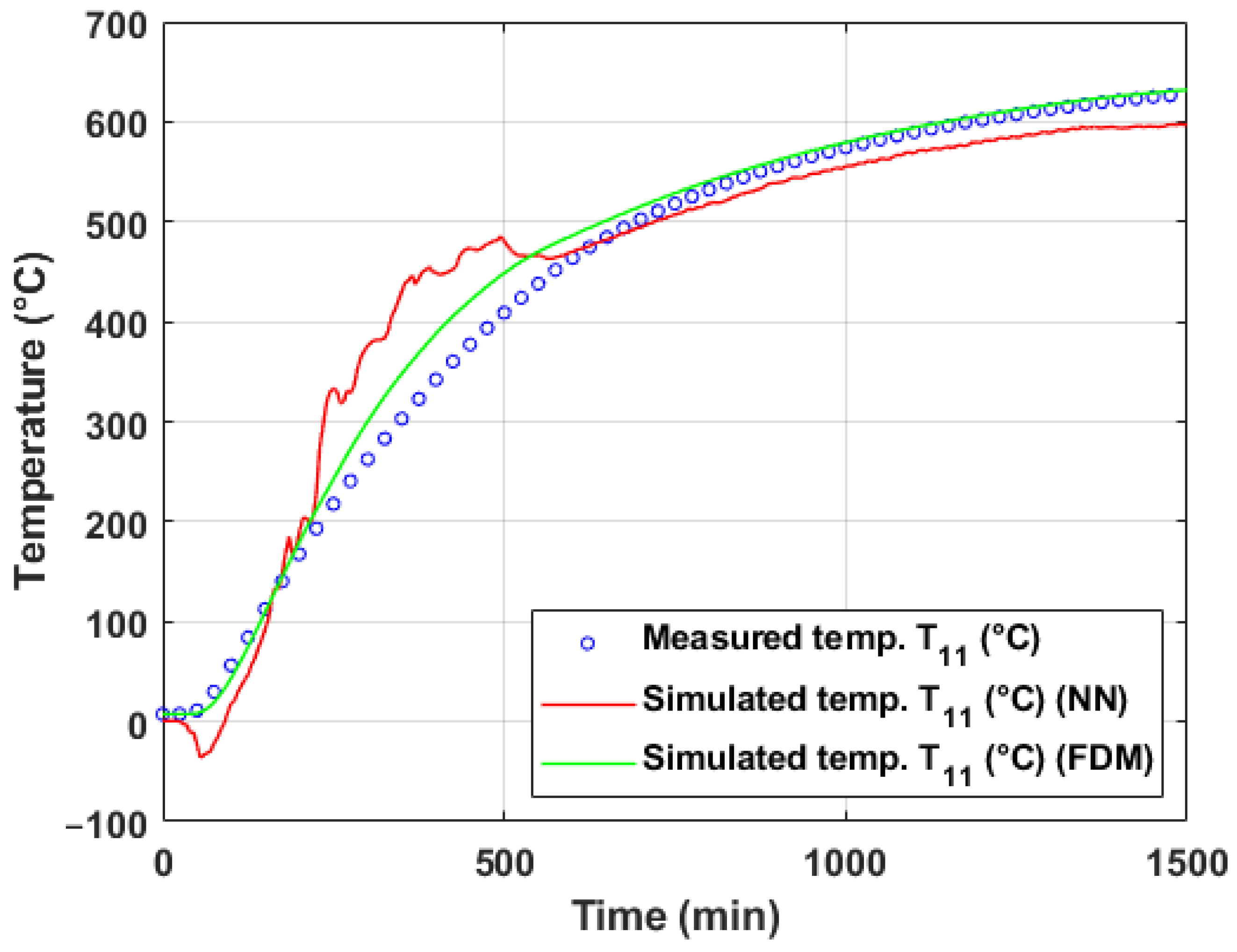
The generalization ability of the trained models was evaluated on unseen test data, and the results are presented in Table 4. Here, the physics-based FDM approach served as a baseline, achieving r y Y = 0.9966 , RRMSE = 4.63%, and PI = 2.3182, demonstrating robust predictive capability without requiring prior training. Among the ML models, MARS (PI = 0.9487 for piecewise-cubic) and RF (PI = 1.0922) provided highly accurate predictions, closely approximating the measured temperature profile. The k-NN model also performed well, but its accuracy decreased slightly compared to the training data (RRMSE = 2.60%). On the other hand, SVR with polynomial and Gaussian kernels failed to generalize, producing very substantial errors and PI values, highlighting their sensitivity to extrapolation beyond the training domain. Neural networks achieved moderate performance (PI = 5.6823), indicating partial overfitting to the training set.
Table 4. Performance of FDM and ML methods in temperature prediction on test data (operational experiment #1).
TemperatureMethod r yY r yY 2 MSEMAPE (%)RMSERRMSE (%)PIMax. Deviation (°C)
T 11 FDM0.99660.9933415.23105.445920.37724.62862.318245.8609
SVR (linear kernel)0.98620.97271001.979325.110131.65417.19013.6199111.7091
SVR (Gaussian kernel)0.96850.93792870.507016.726353.577112.16986.1824311.7023
SVR (polynomial kernel)0.57190.3270118,449,324.536819,275.161910,883.44272472.13071572.747345,295.0617
Feed-forward NN0.96640.93402419.876221.699449.192211.17385.6823131.7777
MARS (piecewise-linear)0.99890.997976.27423.95218.73351.98380.992449.1798
MARS (piecewise-cubic)0.99900.998069.71273.39338.34941.89650.948743.7511
k-NN regression0.99820.9965130.77271.799111.43562.59751.299955.2761
RF0.99880.997792.37131.82439.61102.18311.092253.9474
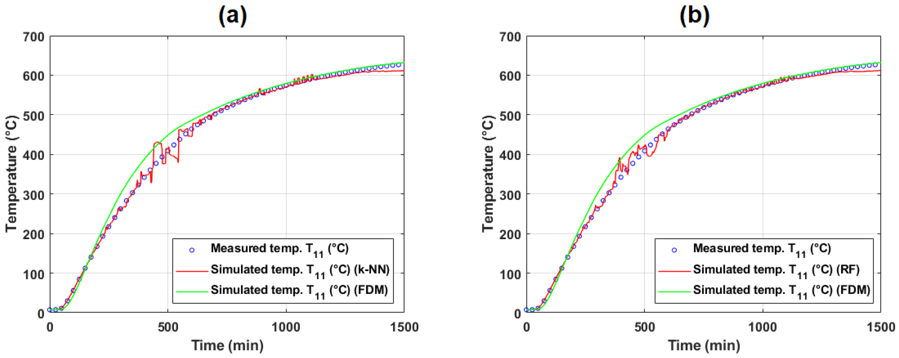
Figure 22, Figure 23, Figure 24 and Figure 25 illustrate the predicted (simulated) inner temperature T 11 compared to measured values for each modeling approach. These plots demonstrate the ability of certain ML models (e.g., RF and MARS) to reproduce the thermal behavior with high fidelity. In contrast, others (e.g., SVR with a polynomial kernel) exhibit considerable deviations, especially during heating and cooling phases.
The examples of mathematical equations for the selected MARS models, including all basis functions, are provided in Appendix B (see Equations (A5) and (A6). These models are portable and can be easily implemented in monitoring systems. The outputs from the MARS models are shown in Figure 24a,b.

5.2.2. Evaluation of Model Performance on Training and Test Data (Operational Experiment #2)

The detailed numerical results for the ML models applied to the training dataset from operational experiment #2 are presented in Appendix C (see Table A5). Both temperatures T 2 and T 8 were modeled simultaneously. Similar to the previous experiment, k-NN and RF achieved nearly perfect predictions, with correlation coefficients approaching unity and extremely low errors (e.g., PI values below 0.3). MARS models (piecewise-linear and piecewise-cubic) also demonstrated excellent fitting capabilities, with r y Y > 0.998 and RRMSE under 3%. SVR with a Gaussian kernel achieved reasonable accuracy but performed worse than MARS and ensemble methods. SVR with a polynomial kernel again struggled with overfitting, as indicated by substantial errors and high PI values. A neural network with the structure 4–9–1–1 demonstrated acceptable performance for T 2 but failed for T 8 , where r y Y 2 = 0.4796 and the PI exceeded 21, indicating instability in learning for some configurations.
The test dataset results, shown in Table 5, demonstrate the generalization performance of both physics-based and ML approaches. The FDM model achieved robust predictions with r y Y > 0.997 for both T 2 and T 8 , and PI values around 1.0, confirming its capability to simulate inner coil temperatures without prior training. Among ML methods, RF and k-NN maintained high accuracy on unseen data, with PI values below 1.0 and maximum deviations comparable to FDM. MARS models also performed well, while SVR with a polynomial kernel exhibited significant errors and was unable to generalize effectively. Neural networks performed moderately on T 2 but showed poor accuracy for T 8 , consistent with their training results.
Table 5. Performance of FDM and ML methods in temperature prediction on test data (operational experiment #2).
TemperatureMethod r yY r yY 2 MSEMAPE (%)RMSERRMSE (%)PIMax. Deviation (°C)
T 2 FDM0.99740.9948359.64625.029118.96434.56072.283347.0768
SVR (linear kernel)0.98140.96321980.165128.222344.499010.70155.4009212.8222
SVR (Gaussian kernel)0.99790.9957773.137113.708627.80536.68693.347053.4657
SVR (polynomial kernel)0.96490.931130,436.939864.0292174.461941.956221.3525346.2543
Feed-forward NN0.98290.96611823.375610.240242.701010.26915.1789209.2889
MARS (piecewise-linear)0.99880.9975135.78573.770411.65272.80241.402084.7990
MARS (piecewise-cubic)0.99840.9969170.13033.900513.04343.13681.569697.9619
k-NN regression0.99940.998865.85020.87718.11481.95150.976182.5804
RF0.99950.999056.21551.19987.49771.80310.901850.8717
T 8 FDM0.99940.998777.00312.19118.77512.06831.034523.8051
SVR (linear kernel)0.98420.96861513.877026.128338.90869.17094.6220195.2460
SVR (Gaussian kernel)0.99790.9958640.387911.843425.30595.96472.985547.1678
SVR (polynomial kernel)0.96270.92683936.602129.786162.742314.78867.5349155.9811
Feed-forward NN0.69250.479624,952.902977.2680157.964937.233021.9985385.5039
MARS (piecewise-linear)0.99840.9968157.30744.127112.54222.95631.479362.6750
MARS (piecewise-cubic)0.99780.9956211.92015.178614.55753.43131.717577.9930
k-NN regression0.99930.998762.76300.90317.92231.86730.934081.5399
RF0.99940.998858.97271.21717.67941.81010.905351.5673
Figure 26 and Figure 27 in the main text, and Figure A1 and Figure A2 in Appendix C, illustrate the predicted inner temperature T 2 versus the measured values across different models. These plots highlight the strong predictive capability of FDM, MARS, k-NN, and RF, which closely follow the real temperature profile. In contrast, SVR and neural networks exhibit larger deviations, particularly during rapid heating and cooling phases.
The examples of mathematical equations for the selected MARS models, including all basis functions, are provided in Appendix B (see Equations (A7) and (A8). These models can be easily implemented in monitoring systems. The outputs from the MARS models are presented in plots (see Figure A2a,b).

5.2.3. Discussion of Model Generalization and Experimental Variability

The comparative analysis of operational experiments #1 and #2 provides valuable insights into the generalization capacity of physics-based and data-driven approaches for modeling inner temperatures during steel coil annealing.
The finite difference method (FDM), a physics-based model grounded in the governing heat transfer equations, consistently exhibits high predictive accuracy across both experiments (see Table 4 and Table 5). It achieved correlation coefficients r y Y > 0.997 and relatively low performance index (PI) values (around 1.0), demonstrating robustness to variations in coil dimensions and stacking configurations. This robustness is expected, as FDM inherently accounts for the physical principles and boundary conditions of the annealing process. However, its computational cost and dependency on accurate material parameters and initial/boundary conditions remain notable limitations.
In contrast, machine learning (ML) models showed more variable performance between experiments. In operational experiment #1, ensemble methods like the random forest (RF) and non-parametric algorithms such as k-nearest neighbors (k-NN) achieved excellent results on both training and test datasets, with PI values often below 1.5 and maximum deviations comparable to FDM. The multivariate adaptive regression splines (MARS) models also performed well, achieving r y Y > 0.998 and low relative root mean square error (RRMSE) values less than 3%.
However, in operational experiment #2, the performance of some ML models deteriorated, particularly for the prediction of T 8 . Neural networks (NNs), which performed moderately on T 2 in the same experiment, failed to capture the dynamics of T 8 , with r y Y 2 = 0.4796 and a PI exceeding 21 (see Table A5). Similarly, support vector regression (SVR) with polynomial kernels exhibited poor generalization, producing large errors and significant deviations during heating and cooling phases (Figure 26). This behavior suggests a tendency for overfitting in the presence of complex or insufficiently diverse training data.
Several factors may explain the observed variability:
  • Differences in experimental conditions: The two experiments featured distinct coil geometries, stacking configurations (four coils in experiment #1 vs. three in experiment #2), and convective ring placements, which likely altered heat transfer patterns within the stacks. Since ML models learn from data patterns rather than physical laws, they may struggle to extrapolate beyond the training domain if these operational variations are not adequately represented in the training set.
  • Limited number of input observations: Compared to laboratory experiments, operational measurements included fewer surface thermocouples. The reduced spatial resolution of inputs could limit the ML models’ ability to infer the thermal behavior deep within the coil stack, particularly for internal thermocouples such as T 8 .
  • Dataset imbalance and covariate shift: The training datasets were derived from specific annealing cycles. If the test dataset exhibits different dynamics or operating regimes (e.g., heating/cooling rates, atmospheric control), data-driven models may encounter covariate shift, leading to degraded predictive performance.
These findings emphasize that while ML models can achieve excellent accuracy in well-represented training domains, their generalization is not guaranteed under different operational conditions. Physics-based models, such as FDM, although computationally demanding, provide a reliable baseline and are less sensitive to such variability.
To mitigate these issues, several strategies could be explored in future work:
  • Hybrid modeling approaches, combining physics-based models with ML techniques (e.g., physics-informed neural networks or residual learning), to integrate domain knowledge with data-driven flexibility.
  • Data augmentation and inclusion of synthetic datasets generated by physical simulations to enrich the diversity of ML training data and improve extrapolation capabilities.
  • Feature engineering, incorporating additional process parameters (e.g., coil weight, convective ring properties, or atmosphere flow rates) as inputs to the ML models.
  • Cross-validation across different operational datasets to systematically assess model robustness and reduce overfitting.
Overall, these experiments highlight the complementary strengths of physics-based and data-driven approaches. While FDM ensures reliability under varying conditions, ML methods excel in speed and adaptability when trained on sufficiently representative data. The integration of these paradigms holds significant promise for robust and efficient temperature prediction in industrial annealing processes.

5.3. Discussion on Laboratory and Operational Measurements

The combined evaluation of laboratory and operational measurements provides critical insights into the strengths and limitations of both physics-based and machine learning (ML) models. Laboratory experiments, conducted under controlled conditions, enabled the dense placement of thermocouples and the fine-grained measurement of boundary and internal temperatures. This setup facilitated the precise calibration and validation of the finite difference model (FDM), enabling the accurate simulation of heat transfer dynamics. However, in operational experiments, the number of available surface measurements was limited due to practical constraints, such as coil stacking and the configuration of the industrial furnace.
The performance index (PI) values obtained from the testing phase for all experimental scenarios are summarized in Table 6 and visualized in Figure 28. This unified presentation provides a compact yet comprehensive comparison across the considered prediction methods. The results indicate that data-driven models such as MARS, k-NN, and RF generally achieved lower PI values (i.e., better accuracy) compared to the physically based FDM and specific SVR configurations, notably the polynomial kernel variant, which exhibited high variability and occasional large deviations. Neural networks (NN) showed competitive performance in several laboratory experiments but less consistent results in operational scenarios. This consolidated format allows for a straightforward ranking of prediction methods under varying conditions, highlighting their robustness and generalization capabilities.
Despite these differences, both experimental setups confirmed the superior generalization capability of ensemble ML methods (k-NN, and RF) and MARS models, which consistently provided accurate inner temperature predictions. Notably, the FDM showed robust performance in both environments, validating its applicability for online estimation even when material properties and boundary conditions varied slightly.
The observed variability between laboratory and industrial data highlights the importance of model adaptability. While ML models trained on laboratory data performed well in controlled settings, their performance deteriorated under the more complex dynamics of industrial annealing unless retrained with operational data. It underscores the potential of hybrid approaches combining physical modeling with adaptive ML techniques for enhanced robustness across different operating regimes.
Although the laboratory and industrial annealing conditions differ significantly in terms of scale and thermal inertia, the proposed models were independently trained and tested on both datasets. It ensured that the evaluation of model performance considered the specific characteristics and complexities of each setting, including real furnace dynamics and coil mass distribution in industrial conditions.
Although research explicitly focused on temperature prediction in bell-type annealing furnaces is limited, several relevant studies present comparable modeling approaches (see Table 7). These studies have also addressed the challenge of predicting internal coil temperatures during the annealing process. For example, Yang et al. [12] developed an analytical thermal model for bell-type annealing furnaces that considered convection and radiation effects, achieving a relative error of less than 0.5% at the cold spot (≤2.5 °C) and a hot spot error was under 5% (≤25 °C). Similarly, Liao et al. [13] proposed a physics-informed neural network (PINN) framework that combined first-principles heat transfer equations with data-driven learning to predict spatio-temporal temperature fields in manufacturing processes, reporting a mean absolute error (MAE) of 7.2 °C. In the context of hydrogen-based annealing, Haouam et al. [10] implemented a finite difference model calibrated using industrial data, achieving a maximum deviation of 12.4 °C from measured core temperatures. Moreover, Pernía-Espinoza et al. [18] demonstrated a robust neural network model for annealing furnaces, capable of handling noisy industrial datasets with a root mean square error (RMSE) of 8.7 °C. Compared to these results, the models presented in this study, particularly the MARS and random forest approaches, achieved a comparable or lower prediction error, indicating their suitability for online soft-sensing applications in annealing operations.
It should be emphasized that the studies summarized in Table 7 differ in terms of experimental setup, material properties, data availability, and modeling objectives. As such, the reported metrics (e.g., RMSE, MAE, and maximum deviation) are not directly comparable in a strict sense. The intention of this comparison is not to rank the models by accuracy, but rather to illustrate the general range of prediction errors reported in the literature for similar thermal modeling problems. We highlight that some studies, such as [13], focus on additive manufacturing processes, while others, such as [12], employ analytical simplifications. Despite these contextual differences, the comparison provides a valuable benchmark to position our study within the broader research landscape.
Unlike purely physics-based models, hybrid approaches such as Liao et al. [13] using physics-informed neural networks for thermal processes in additive manufacturing showed that combining data-driven corrections with PDE-based core models can reduce prediction errors by over 50% compared to standalone ML surrogates [13]. It supports our findings: ensemble ML models (i.e., RF, k-NN, and MARS) can outperform FDM under well-represented data conditions, but FDM remains competitive and more robust when data variability increases. Together, these comparisons demonstrate that our study aligns well with existing physics-based literature and extends it by highlighting the added value of hybrid and purely data-driven models in industrial annealing contexts.

6. Conclusions

This study presented a comparative analysis of physics-based and machine learning methods for predicting inner temperatures in steel coils during annealing. The finite difference method (FDM) demonstrated reliable performance in both laboratory and industrial settings, providing physically interpretable results without requiring extensive training data. Among the evaluated ML techniques, multivariate adaptive regression splines (MARS), k-nearest neighbors (k-NN), and random forests (RF) achieved superior accuracy and generalization on unseen data (PI < 1.0), making them promising candidates for soft-sensor applications. In contrast, support vector regression (SVR) with polynomial kernels and neural networks showed limitations in handling data variability and exhibited susceptibility to overfitting. Among the evaluated ML techniques, multivariate adaptive regression splines (MARS), k-nearest neighbors (k-NN), and random forests (RF) achieved superior accuracy and generalization on unseen data (PI < 1.0), making them promising candidates for soft-sensor applications. These data-driven models exhibited greater flexibility in capturing complex nonlinear relationships in the input–output space, which likely contributed to their improved predictive performance. Unlike the FDM, which relies on simplified assumptions about heat transfer and material parameters, the ML models were able to implicitly learn patterns from the measurements, adapting more effectively to variations in geometry, sensor placement, and boundary conditions. This is consistent with the detailed analysis provided in Section 5.1 and Section 5.2.
There is no universally optimal modeling approach for predicting steel coil temperature within bell annealing furnaces; each method reflects trade-offs among physical fidelity, adaptability, computational demands, data availability, and interpretability. The technological trend is decisively towards hybrid, physics-informed data-driven models capable of delivering high-fidelity, real-time predictions with reliable adaptation and robustness in practical steel manufacturing settings. Future advances are likely to integrate further sensor-driven “digital twin” frameworks, explainable AI, and uncertainty-aware prediction schemes, thereby enhancing process optimization and quality assurance.
The comparative evaluation across laboratory and industrial datasets revealed consistent strengths and weaknesses of both physics-based and data-driven models. While the finite difference method (FDM) provided physically interpretable predictions and performed robustly across varying experimental setups, specific machine learning models (e.g., MARS, k-NN, and RF) demonstrated superior prediction accuracy when sufficient and representative data were available. These findings emphasize the complementary nature of the two approaches and highlight the potential of hybrid physics-informed data-driven frameworks for real-time soft sensing in steel annealing operations.
However, challenges remain in ensuring robustness under highly variable operational conditions, as well as in integrating these models into real-time control systems. Future work should explore the incorporation of domain knowledge into ML models to improve interpretability and resilience, along with the development of hybrid frameworks that dynamically balance data-driven adaptability with physical model constraints.

Author Contributions

Conceptualization, J.K. and P.F.; data curation, J.K. and P.F.; formal analysis, M.D. and M.L.; methodology, J.K. and P.F.; project administration, J.K.; resources, M.D. and M.L.; supervision, M.D. and M.L.; validation, M.D.; writing—original draft preparation, J.K. and P.F.; writing—review and editing, P.F. All authors have read and agreed to the published version of the manuscript.

Funding

This research was funded by the Slovak Research and Development Agency under contract APVV-22-0508 and by the Scientific Grant Agency of the Ministry of Education, Research, Development, and Youth of the Slovak Republic under contract VEGA 1/0039/24. The article also relates to the objectives of the project proposal VEGA 1/0055/26, currently under evaluation.

Data Availability Statement

The original contributions presented in this study are included in the article. Further inquiries can be directed to the corresponding author.

Conflicts of Interest

The authors declare no conflicts of interest.

Abbreviations

The following abbreviations are used in this manuscript:
PLCProgrammable Logic Controller
OPCOpen Platform Communications
PWMPulse-Width modulation
SMCSliding Mode Control
PIDProportional–Integral–Derivative
PDEPartial Differential Equation
MLMachine Learning
ANNArtificial Neural Network
FDMFinite Difference Method
FEMFinite Element Method
RFRandom Forest
k-NNk-Nearest Neighbors
MAPEMean Absolute Percentage Error
MARSMultivariate Adaptive Regression Splines
BFBasis Function
PCPersonal Computer
NNNeural Network
PIPerformance Index
RMSERoot Mean Squared Error
RRMSERelative RMSE
GCVGeneralized Cross-Validation
SVMSupport Vector Machines
SVRSupport Vector Regression
PINNsPhysics-Informed Neural Networks
ELMExtreme Learning Machines
CBRCase-Based Reasoning
RBFNNRadial Basis Function Neural Networks
x Coil’s surface temperature as input observations
y, y T Target variable (predicted temperature) (°C)
r y Y Correlation coefficient
r y Y 2 Coefficient of determination
T i , j k Temperature at spatial grid node ( i , j ) and time step k (in FDM) (K)
T mer , j Measured temperature at index j (K)
T sim , j Simulated (predicted) temperature by FDM at index j (K)
tTime (s)
Δ τ Time step (s)
λ Thermal conductivity (in FDM context) ( W m 1 K 1 )
α Thermal diffusivity ( m 2 s 1 )
cSpecific heat capacity ( J kg 1 K 1 )
ρ Material density ( kg m 3 )
K Kernel matrix
f ^ Prediction function

Appendix A. Main Approaches for Temperature Modeling in Steel Coil Annealing

Table A1. Comparison of different modeling approaches applicable for estimating temperature in the annealing of steel coils.
ApproachTypeAccuracyComputational
Demand
Real-Time
Capable
InterpretabilityData
Requirements
StrengthsWeaknessesKey
References
Finite
Difference/
Element (FD/FEM)
Physics-basedHighHighFeasible
(optimized)
HighLow/
Medium
Detailed,
spatially resolved,
process simulation
Detailed data
and tuning,
slower
(for large
system sizes)
[7,8,9,81],
[1,2,10,14]
Lumped
Parameter
Models
Physics-basedModerateLowYesModerateLowFast,
applicable to
real-time
control, compact
Misses spatial
gradients,
idealizations
[8]
Analytical/Hybrid
Physics
Physics-basedLow–ModVery LowYesHighLowSimple,
transparent
Oversimplified;
poor under
industrial variability
[8,11,12,13]
Artificial Neural
Networks
(ANN, ELM,
RBFNN, GRNN)
MLModerate–HighModerateYesLowHighCaptures nonlinearity,
adaptive, incremental
learning possible
Opacity, needs
extensive and
curated process
data
[18,19,20,35,82],
[28,29,30],
[21,22,23],
[24,25,26,27]
Ensemble/
Incremental
ML Models
MLHighModerateYesLowHighRobustness to
outliers, adapts over
time
Complexity,
model management
[19,35]
Support Vector
Regression (SVR)
MLModerateModerateYesModerateMediumEffective with
small-to-midsize,
nonlinear datasets
Parameter tuning,
not yet dominant
in this domain
[31,32,33]
Bayesian Belief
Network + CBR
ML/
Probabilistic
Moderate–HighModerateYesModerate–HighHighProbabilistic
predictions, reliability
estimation
Integration complexity,
data intensive
[34]
System Identification
+ Physics
HybridHighLow–ModerateYesModerateMediumCombines best
of both—realistic,
adaptive
Model structure
design can be tricky
[8]

Appendix B. Examples of MARS Models for Temperature Prediction

Appendix B.1. Examples of MARS Models Tested on Laboratory Experiment #2

The result of the piecewise-linear-type of the MARS model with all its basis functions for simulating (prediction) of temperature T 2 (°C) is as follows:
y T 2 = 154.91 0.28607 × BF 1 + 0.38562 × BF 2 + 0.27938 × BF 3 0.37726 × BF 4 + 1.1239 × BF 5 1.2014 × BF 6 0.14587 × BF 7 + 0.032673 × BF 8 ,
where BF1 = max(0, x 1 − 363.3), BF2 = max(0, 363.3 − x 1 ), BF3 = max(0, x 14 − 339.42), BF4 = max(0, 339.42 − x 14 ), BF5 = max(0, x 5 − 146.1), BF6 = max(0, 146.1 − x 5 ), BF7 = max(0, x 12 − 132.63), and BF8 = max(0, 132.63 − x 12 ) are basis functions according to (14).
The piecewise-cubic MARS model of temperature T 2 (°C) is as follows:
y T 2 = 143.41 0.32723 × BF 1 + 0.43114 × BF 2 + 0.2786 × BF 3 0.36558 × BF 4 + 1.182 × BF 5 1.2692 × BF 6 0.15753 × BF 7 + 0.03824 × BF 8 ,
where BF1 = C( x 1   | +1, 192.6, 363.3, 533.5), BF2 = C( x 1   | −1, 192.6, 363.3, 533.5), BF3 = C( x 14   | +1, 179.02, 339.42, 525.56), BF4 = C( x 14   | −1, 179.02, 339.42, 525.56), BF5 = C( x 5   | +1, 84.55, 146.1, 429.55), BF6 = C( x 5   | −1, 84.55, 146.1, 429.55), BF7 = C( x 12   | +1, 78.215, 132.63, 430.56), and BF8 = C( x 12   | −1, 78.215, 132.63, 430.56) are basis functions according to (15).

Appendix B.2. Examples of MARS Models Tested on Laboratory Experiment #4

The result of the piecewise-linear type of the MARS model with all its basis functions for simulating (prediction) of temperature T 2 (°C) is as follows:
y T 2 = 154.91 0.28607 × BF 1 + 0.38562 × BF 2 + 0.27938 × BF 3 0.37726 × BF 4 + 1.1239 × BF 5 1.2014 × BF 6 0.14587 × BF 7 + 0.032673 × BF 8 ,
where BF1 = max(0, x 1 − 363.3), BF2 = max(0, 363.3 − x 1 ), BF3 = max(0, x 14 − 339.42), BF4 = max(0, 339.42 − x 14 ), BF5 = max(0, x 5 − 146.1), BF6 = max(0, 146.1 − x 5 ), BF7 = max(0, x 12 − 132.63), and BF8 = max(0, 132.63 − x 12 ) are basis functions according to (14).
The piecewise-cubic MARS model of temperature T 2 (°C) is as follows:
y T 2 = 143.41 0.32723 × BF 1 + 0.43114 × BF 2 + 0.2786 × BF 3 0.36558 × BF 4 + 1.182 × BF 5 1.2692 × BF 6 0.15753 × BF 7 + 0.03824 × BF 8 ,
where BF1 = C( x 1   | +1, 192.6, 363.3, 533.5), BF2 = C( x 1   | −1, 192.6, 363.3, 533.5), BF3 = C( x 14   | +1, 179.02, 339.42, 525.56), BF4 = C( x 14   | −1, 179.02, 339.42, 525.56), BF5 = C( x 5   | +1, 84.55, 146.1, 429.55), BF6 = C( x 5   | −1, 84.55, 146.1, 429.55), BF7 = C( x 12   | +1, 78.215, 132.63, 430.56), and BF8 = C( x 12   | −1, 78.215, 132.63, 430.56) are basis functions according to (15).

Appendix B.3. Examples of MARS Models Tested on Operational Experiment #1

The result of the piecewise-linear type of the MARS model with all its basis functions for simulating (prediction) of temperature T 11 (°C) is as follows:
y T 11 = 211.18 + 2.2921 × BF 1 0.52266 × BF 2 1.1905 × BF 3 0.45447 × BF 4 0.057663 × BF 5 + 0.035088 × BF 6 0.00012454 × BF 7 + 0.0065221 × BF 8 0.050968 × BF 9 + 0.0011432 × BF 10 + 8.0668 × BF 11 + 0.040567 × BF 12 + 0.032755 × BF 13 + 0.0007102 × BF 14 + 0.017968 × BF 15 + 1.3878 × 10 6 × BF 16 1.2727 × 10 5 × BF 17 0.0019355 × BF 18 0.00079015 × BF 19 ,
where BF1 = max(0, x 4 − 488.33), BF2 = max(0, 488.33 − x 4 ), BF3 = max(0, x 1 − 556.7), BF4 = max(0, 556.7 − x 1 ), BF5 = BF3 × max(0, x 4 − 523.39), BF6 = BF3 × max(0, 523.39 − x 4 ), BF7 = BF5 × max(0, x 3 − 546.59), BF8 = BF5 × max(0, 546.59 − x 3 ), BF9 = BF2 × max(0, x 1 − 556.05), BF10 = BF2 × max(0, 556.05 − x 1 ), BF11 = max(0, x 4 − 543.16), BF12 = BF11 × max(0, x 1 − 625.03), BF13 = BF11 × max(0, 625.03 − x 1 ), BF14 = BF13 × max(0, x 5 − 637.24), BF15 = BF13 × max(0, 637.24 − x 5 ), BF16 = BF7 × max(0, x 2 − 606.98), BF17 = BF7 × max(0, 606.98 − x 2 ), BF18 = BF15 × max(0, x 3 − 566.05), and BF19 = BF15 × max(0, 566.05 − x 3 ) are basis functions according to (14).
The piecewise-cubic MARS model of temperature T 11 (°C) is as follows:
y T 11 = 226.8 + 0.99956 × BF 1 0.66344 × BF 2 0.093987 × BF 3 0.28438 × BF 4 0.04174 × BF 5 0.015523 × BF 6 + 0.00022397 × BF 7 + 0.014314 × BF 8 + 0.00043347 × BF 9 + 0.00098295 × BF 10 + 5.6283 × BF 11 0.010307 × BF 12 + 0.11776 × BF 13 + 0.00030566 × BF 14 + 0.029768 × BF 15 1.0109 × 10 6 × BF 16 1.4331 × 10 5 × BF 17 0.0019268 × BF 18 + 0.00092708 × BF 19 ,
where BF1 = C( x 4   | +1, 247.84, 488.33, 505.86), BF2 = C( x 4   | −1, 247.84, 488.33, 505.86), BF3 = C( x 1   | +1, 556.38, 556.7, 590.86), BF4 = C( x 1   | −1, 556.38, 556.7, 590.86), BF5 = BF3 × C( x 4   | +1, 505.86, 523.39, 533.27), BF6 = BF3 × C( x 4   | −1, 505.86, 523.39, 533.27), BF7 = BF5 × C( x 3   | +1, 277.31, 546.59, 556.32), BF8 = BF5 × C( x 3   | −1, 277.31, 546.59, 556.32), BF9 = BF2 × C( x 1   | +1, 282.29, 556.05, 556.38), BF10 = BF2 × C( x 1   | −1, 282.29, 556.05, 556.38), BF11 = C( x 4   | +1, 533.27, 543.16, 598.44), BF12 = BF11 × C( x 1   | +1, 590.86, 625.03, 644.72), BF13 = BF11 × C( x 1   | −1, 590.86, 625.03, 644.72), BF14 = BF13 × C( x 5   | +1, 323.08, 637.24, 657.49), BF15 = BF13 × C( x 5   | −1, 323.08, 637.24, 657.49), BF16 = BF7 × C( x 2   | +1, 307.56, 606.98, 631.73), BF17 = BF7 × C( x 2   | −1, 307.56, 606.98, 631.73), BF18 = BF15 × C( x 3   | +1, 556.32, 566.05, 609.4), and BF19 = BF15 × C( x 3   | −1, 556.32, 566.05, 609.4) are basis functions according to (15).

Appendix B.4. Examples of MARS Models Tested on Operational Experiment #2

The result of the piecewise-linear type of the MARS model with all its basis functions for simulating (prediction) of temperature T 2 (°C) is as follows:
y T 2 = 1754.2 + 13.225 × BF 1 5.0658 × BF 2 2.7491 × BF 3 0.29057 × BF 4 + 0.75102 × BF 5 + 0.0088357 × BF 6 0.0078798 × BF 7 + 0.44525 × BF 8 0.029526 × BF 9 + 0.0083005 × BF 10 0.017713 × BF 11 0.00046808 × BF 12 + 0.0090777 × BF 13 + 0.0022618 × BF 14 0.00013097 × BF 15 0.00013787 × BF 16 + 0.00076145 × BF 17 0.019479 × BF 18 ,
where BF1 = max(0, x 3 − 656.08), BF2 = max(0, 656.08 − x 3 ), BF3 = max(0, x 4 − 243.88), BF4 = max(0, x 2 − 203.47), BF5 = max(0, 203.47 − x 2 ), BF6 = BF2 × max(0, x 4 − 233.05), BF7 = BF2 × max(0, 233.05 − x 4 ), BF8 = max(0, x 4 − 439.04), BF9 = max(0, 439.04 − x 4 ) × max(0, x 3 − 514.48), BF10 = max(0, 439.04 − x 4 ) × max(0, 514.48 − x 3 ), BF11 = BF4 × max(0, x 3 − 659.1), BF12 = BF4 × max(0, 659.1 − x 3 ), BF13 = BF2 × max(0, x 1 − 488.9), BF14 = BF2 × max(0, 488.9 − x 1 ), BF15 = BF13 × max(0, x 4 − 509.89), BF16 = BF13 × max(0, 509.89 − x 4 ), BF17 = BF8 × max(0, x 1 − 649.85), and BF18 = BF8 × max(0, 649.85 − x 1 ) are basis functions according to (14).
The piecewise-cubic MARS model of temperature T 2 (°C) is as follows:
y T 2 = 1740.3 + 7.1879 × BF 1 4.8394 × BF 2 1.6664 × BF 3 0.76534 × BF 4 + 1.1444 × BF 5 + 0.0055135 × BF 6 0.0069839 × BF 7 0.37686 × BF 8 0.0021144 × BF 9 + 0.0072109 × BF 10 0.0043611 × BF 11 + 0.00062418 × BF 12 + 0.012242 × BF 13 + 0.0019414 × BF 14 0.00012884 × BF 15 0.00018178 × BF 16 0.0016537 × BF 17 0.022726 × BF 18 ,
where BF1 = C( x 3   | +1, 585.28, 656.08, 657.59), BF2 = C( x 3   | −1, 585.28, 656.08, 657.59), BF3 = C( x 4   | +1, 238.47, 243.88, 341.46), BF4 = C( x 2   | +1, 113, 203.47, 458.41), BF5 = C( x 2   | −1, 113, 203.47, 458.41), BF6 = BF2 × C( x 4   | +1, 132.65, 233.05, 238.47), BF7 = BF2 × C( x 4   | −1, 132.65, 233.05, 238.47), BF8 = C( x 4   | +1, 341.46, 439.04, 474.46), BF9 = C( x 4   | −1, 341.46, 439.04, 474.46) × C( x 3   | +1, 266.6, 514.48, 585.28), BF10 = C( x 4   | −1, 341.46, 439.04, 474.46) × C( x 3   | −1, 266.6, 514.48, 585.28), BF11 = BF4 × C( x 3   | +1, 657.59, 659.1, 683.96), BF12 = BF4 × C( x 3   | −1, 657.59, 659.1, 683.96), BF13 = BF2 × C( x 1   | +1, 256.36, 488.9, 569.37), BF14 = BF2 × C( x 1   | −1, 256.36, 488.9, 569.37), BF15 = BF13 × C( x 4   | +1, 474.46, 509.89, 612.36), BF16 = BF13 × C( x 4   | −1, 474.46, 509.89, 612.36), BF17 = BF8 × C( x 1   | +1, 569.37, 649.85, 682), and BF18 = BF8 × C( x 1   | −1, 569.37, 649.85, 682) are basis functions according to (15).

Appendix C. Performance of Prediction Models

Appendix C.1. Performance of Prediction Models Based on Laboratory Measurements

Table A2. Performance of ML methods in training data fitting (experiment #2).
TemperatureMethod r yY r yY 2 MSEMAPE (%)RMSERRMSE (%)PIMax. Deviation (°C)Training Time (s)
T 2 SVR (linear kernel)0.99910.9982206.35428.473914.36502.97761.489526.78580.5078
SVR (Gaussian kernel)0.99880.9976493.020812.653122.20414.60252.302626.88942.7228
SVR (polynomial kernel)0.99600.99201255.011827.039135.42617.34313.679091.2727204.8109
Feed-forward NN0.99910.998397.81523.06659.89022.05001.025527.30362.3030
MARS (piecewise-linear)0.99990.99998.44391.07522.90580.60230.301218.5558277.0577
MARS (piecewise-cubic)0.99990.99997.62071.06132.76060.57220.286114.4765277.2751
k-NN regression1.00001.00000.00590.02110.07690.01590.00800.84200.0005
RF1.00001.00000.23640.31850.48620.10080.05043.7641408.6441
T 3 SVR (linear kernel)0.99960.9991327.139710.795618.08703.73411.867527.71610.5069
SVR (Gaussian kernel)0.99880.9975513.949513.035022.67054.68042.341727.39271.8591
SVR (polynomial kernel)0.99500.99012681.704047.755951.785210.69125.3589148.3949206.2741
Feed-forward NN0.99920.998489.06723.66829.43751.94840.974632.45082.4091
MARS (piecewise-linear)0.99990.999810.99231.50933.31550.68450.342321.8608172.7441
MARS (piecewise-cubic)0.99990.999813.46251.69483.66910.75750.378825.5280175.0099
k-NN regression1.00001.00000.00600.02110.07730.01600.00800.84800.0005
RF1.00001.00000.36450.31670.60380.12460.06237.4659412.1197
T 4 SVR (linear kernel)0.99870.9973293.54006.260917.13303.57411.788229.60530.5071
SVR (Gaussian kernel)0.99860.9971606.661314.965324.63055.13812.570929.67043.1536
SVR (polynomial kernel)0.98050.96149683.263692.908198.403620.527710.3649237.4634204.4006
Feed-forward NN0.99900.9980115.83094.118510.76252.24511.123144.43252.5095
MARS (piecewise-linear)0.99990.999813.79111.31123.71360.77470.387417.8987109.6908
MARS (piecewise-cubic)0.99990.999813.78231.28723.71250.77440.387217.7504107.7261
k-NN regression1.00001.00000.00580.02210.07640.01590.00800.80800.0005
RF1.00001.00000.46200.36260.67970.14180.07095.9890418.2398
Table A3. Performance of ML methods in training data fitting (experiment #4).
TemperatureMethod r yY r yY 2 MSEMAPE (%)RMSERRMSE (%)PIMax. Deviation (°C)Training Time (s)
T 2 SVR (linear kernel)0.99920.9984210.87587.610614.52162.92481.463027.46290.5500
SVR (Gaussian kernel)0.99830.9966541.795613.207323.27654.68822.346127.49894.3830
SVR (polynomial kernel)0.99430.98864297.106522.825965.552313.20306.6204125.2540210.6607
Feed-forward NN0.99530.9905555.476511.785823.56854.74702.379166.32792.2936
MARS (piecewise-linear)1.00000.99993.16170.83511.77810.35810.17916.9960164.8469
MARS (piecewise-cubic)1.00001.00002.65420.79311.62920.32810.16416.6689164.9850
k-NN regression1.00001.00000.00540.02520.07320.01470.00740.64000.0007
RF1.00001.00000.40190.34950.63390.12770.06382.3455502.0956
T 3 SVR (linear kernel)0.99970.9993454.094310.162221.30954.31062.155628.67310.5874
SVR (Gaussian kernel)0.99830.9966590.797413.582224.30634.91682.460528.71692.9958
SVR (polynomial kernel)0.97440.9494118,618.1770158.3507344.409969.668835.2868449.8708236.9107
Feed-forward NN0.99950.998965.08403.87388.06751.63190.816233.20732.3110
MARS (piecewise-linear)1.00000.99995.20530.95432.28150.46150.230819.178696.7913
MARS (piecewise-cubic)1.00000.99995.75261.07142.39850.48520.242620.265094.9964
k-NN regression1.00001.00000.00520.02520.07190.01460.00730.56000.0008
RF1.00001.00000.31660.33520.56260.11380.05693.0145410.0908
T 4 SVR (linear kernel)0.99850.9970392.70638.138819.81684.05062.026830.6820538.9285
SVR (Gaussian kernel)0.99810.9963695.138816.276226.36555.38912.697130.71385.8669
SVR (polynomial kernel)0.99460.98929786.076629.430298.924620.220310.1376174.3081248.8493
Feed-forward NN0.98010.96052445.782045.724949.454810.10865.1052188.10401.6127
MARS (piecewise-linear)0.99990.999810.14561.28633.18520.65110.32559.717694.2215
MARS (piecewise-cubic)0.99990.999810.14221.28893.18470.65100.32559.329794.3742
k-NN regression1.00001.00000.00500.02610.07090.01450.00720.36000.0009
RF1.00001.00000.22900.29990.47850.09780.04892.6471413.7298

Appendix C.2. Performance of Prediction Models Based on Operational Measurements

Table A4. Performance of ML methods in training data fitting (operational experiment #1).
TemperatureMethod r yY r yY 2 MSEMAPE (%)RMSERRMSE (%)PIMax. Deviation (°C)Training Time (s)
T 11 SVR (linear kernel)0.98670.9735979.309124.142831.29397.12813.5880111.99111.1883
SVR (Gaussian kernel)0.99770.9954188.730813.711413.73793.12921.566436.77330.4382
SVR (polynomial kernel)0.57530.3309119,880,717.717118,858.849010,949.00532493.94461583.188245,321.880455.9787
Feed-forward NN0.96840.93782272.689121.299647.672710.85885.5165134.96831.6135
MARS (piecewise-linear)0.99910.998264.41113.66318.02571.82810.914451.491718.5185
MARS (piecewise-cubic)0.99910.998167.54973.30568.21891.87210.936547.534818.4478
k-NN regression1.00001.00001.15670.43671.07550.24500.122516.87350.0006
RF1.00000.99992.66620.71201.63290.37190.186018.484897.7661
Table A5. Performance of ML methods in training data fitting (operational experiment #2).
TemperatureMethod r yY r yY 2 MSEMAPE (%)RMSERRMSE (%)PIMax. Deviation (°C)Training Time (s)
T 2 SVR (linear kernel)0.98140.96311962.297528.074344.297810.69295.3967212.83894.9031
SVR (Gaussian kernel)0.99780.9957795.860713.762128.21106.80973.408535.21211.0933
SVR (polynomial kernel)0.96580.932827,545.333162.3341165.967940.062320.3795350.013792.7547
Feed-forward NN0.98330.96681762.290310.233641.979610.13335.1094209.97251.4795
MARS (piecewise-linear)0.99860.9973142.87233.824911.95292.88531.443691.583359.0619
MARS (piecewise-cubic)0.99850.9970161.43533.938612.70573.06701.5347104.936159.2119
k-NN regression1.00001.00001.32210.19451.14980.27760.138812.38830.0005
RF1.00000.99995.03370.51312.24360.54160.270851.0764167.8558
T 8 SVR (linear kernel)0.98420.96871494.474925.854038.65849.14484.6088195.28253.5057
SVR (Gaussian kernel)0.99580.9979651.827511.901625.53096.03943.022932.55040.9362
SVR (polynomial kernel)0.96170.92484125.710929.854064.231715.19427.7456159.470393.7252
Feed-forward NN0.69250.479624,661.524576.8499157.039937.148421.9483389.52800.7673
MARS (piecewise-linear)0.99820.9964169.80304.342213.03083.08251.542679.900648.1415
MARS (piecewise-cubic)0.99780.9955211.63255.221114.54763.44131.722679.073447.7717
k-NN regression1.00001.00001.26950.21561.12670.26650.133312.28960.0005
RF0.99990.99995.74140.56812.39610.56680.283465.3652171.1530
Figure A1. Measured and simulated temperature T 2 using FDM and NN (operational experiment #2).
Metals 15 00932 g0a1
Figure A2. Measured and simulated temperature T 2 using FDM and MARS (operational experiment #2): (a) MARS, piecewise-linear; (b) MARS, piecewise-cubic.
Metals 15 00932 g0a2

References

  1. Durdán, M.; Kačur, J. System for indirect measurement of the heat flows at annealing of the steel coils. Acta Metall. Slovaca 2013, 19, 112–121. [Google Scholar] [CrossRef]
  2. Durdán, M.; Mojžišová, A.; Laciak, M.; Kačur, J. System for indirect temperature measurement in annealing process. Measurement 2014, 47, 911–918. [Google Scholar] [CrossRef]
  3. Kačur, J.; Durdán, M.; Laciak, M.; Flegner, P. Soft-Sensing in Batch Annealing Based on Finite Differential Method and Support Vector Regression. Adv. Sci. Technol. Res. J. 2019, 13, 70–86. [Google Scholar] [CrossRef]
  4. Couchet, C.; Bonnet, F.; Teixeira, J.; Allain, S.Y.P. Numerical Investigations of Phase Transformations Controlled by Interface Thermodynamic Conditions during Intercritical Annealing of Steels. Metals 2023, 13, 1288. [Google Scholar] [CrossRef]
  5. Yang, Y.; Ma, X.; Lu, H.; Zhao, Z. Effect of Annealing Temperature on Microstructure and Properties of DH Steel and Optimization of Hole Expansion Property. Metals 2024, 14, 791. [Google Scholar] [CrossRef]
  6. Chu, X.; Zhou, F.; Liu, L.; Xu, X.; Ma, X.; Li, W.; Zhao, Z. Evolution of Microstructure, Properties, and Fracture Behavior with Annealing Temperature in Complex Phase Steel with High Formability. Metals 2024, 14, 380. [Google Scholar] [CrossRef]
  7. Sahay, S.S.; Kumar, A.M. Applications of Integrated Batch Annealing Furnace Simulation. Mater. Manuf. Process. 2002, 17, 439–453. [Google Scholar] [CrossRef]
  8. Tian, Y.; Hou, C.; Gao, F. Mathematical Model of a Continuous Galvanizing Annealing Furnace. Dev. Chem. Eng. Miner. Process. 2000, 8, 359–374. [Google Scholar] [CrossRef]
  9. Kostúr, K.; Laciak, M.; Truchlý, M. Systémy Nepriameho Merania; TU: Košice, Slovakia, 2005. [Google Scholar]
  10. Haouam, A.; Bigerelle, M.; Merzoug, B. Simplex Enhanced Numerical Modeling of the Temperature Distribution in a Hydrogen Cooled Steel Coil Annealing Process. Procedia Eng. 2016, 157, 50–57. [Google Scholar] [CrossRef]
  11. Durdán, M.; Stehlíková, B.; Pástor, M.; Kačur, J.; Laciak, M.; Flegner, P. Research of annealing process in laboratory conditions. Measurement 2015, 73, 607–618. [Google Scholar] [CrossRef]
  12. Yang, X.J.; Dai, F.X.; Bao, X.J.; Chen, G.; Zhang, L.; Li, Y.R. Study of heat transfer model and buried thermocouple test of bell-type annealing furnace based on thermal equilibrium. Sci. Rep. 2025, 15, 13362. [Google Scholar] [CrossRef]
  13. Liao, S.; Xue, T.; Jeong, J.; Webster, S.; Ehmann, K.; Cao, J. Hybrid thermal modeling of additive manufacturing processes using physics-informed neural networks for temperature prediction and parameter identification. Comput. Mech. 2023, 72, 499–512. [Google Scholar] [CrossRef]
  14. Kostúr, K. Process check of annealing process of coiled sheets by indirect measurement. Metalurgija 2017, 56, 229–232. [Google Scholar]
  15. Zhou, X.; Xu, J.; Meng, L.; Wang, W.; Zhang, N.; Jiang, L. Machine-Learning-Assisted Composition Design for High-Yield-Strength TWIP Steel. Metals 2024, 14, 952. [Google Scholar] [CrossRef]
  16. Bachmann, B.I.; Müller, M.; Britz, D.; Staudt, T.; Mücklich, F. Reproducible Quantification of the Microstructure of Complex Quenched and Quenched and Tempered Steels Using Modern Methods of Machine Learning. Metals 2023, 13, 1395. [Google Scholar] [CrossRef]
  17. Tiwari, S.; Heo, S.; Park, N.; Reddy, N.G.S. Modeling Mechanical Properties of Industrial C-Mn Cast Steels Using Artificial Neural Networks. Metals 2025, 15, 790. [Google Scholar] [CrossRef]
  18. Pernía-Espinoza, A.; Castejón-Limas, M.; González-Marcos, A.; Lobato-Rubio, V. Steel annealing furnace robust neural network model. Ironmak. Steelmak. 2005, 32, 418–426. [Google Scholar] [CrossRef]
  19. Tian, H.X.; Mao, Z.Z. An Ensemble ELM Based on Modified AdaBoost.RT Algorithm for Predicting the Temperature of Molten Steel in Ladle Furnace. IEEE Trans. Autom. Sci. Eng. 2010, 7, 73–80. [Google Scholar] [CrossRef]
  20. Qiao, L.; Zhu, J.; Wang, Y. Machine Learning-Aided Process Design: Modeling and Prediction of Transformation Temperature for Pearlitic Steel. Steel Res. Int. 2021, 93, 1–10. [Google Scholar] [CrossRef]
  21. Bhadeshia, H.K.D.H. Neural Networks in Materials Science. ISIJ Int. 1999, 39, 966–979. [Google Scholar] [CrossRef]
  22. Çöl, M.; Ertunç, H.M.; Yılmaz, M. An artificial neural network model for toughness properties in microalloyed steel in consideration of industrial production conditions. Mater. Des. 2007, 28, 488–495. [Google Scholar] [CrossRef]
  23. Dehghani, K.; Shafiei, A. Predicting the bake hardenability of steels using neural network modeling. Mater. Lett. 2008, 62, 173–178. [Google Scholar] [CrossRef]
  24. Garrett, P.H. Neural network directed steel annealing. In High Performance Instrumentation and Automation; CRC Press: Boca Raton, FL, USA, 2018; pp. 209–216. [Google Scholar] [CrossRef]
  25. Chen, M.Y.; Linkens, D.A. A systematic neuro-fuzzy modeling framework with application to material property prediction. IEEE Trans. Syst. Man Cybern. Part B (Cybern.) 2001, 31, 781–790. [Google Scholar] [CrossRef]
  26. Chen, M.Y.; Linkens, D.A.; Bannister, A. Numerical analysis of factors influencing Charpy impact properties of TMCR structural steels using fuzzy modelling. Mater. Sci. Technol. 2004, 20, 627–633. [Google Scholar] [CrossRef]
  27. Jones, D.M. The Modelling of Mechanical Properties of Steel from Processing Parameters at the Port Talbot Hot Strip Mill. Engineering Doctorate Thesis, Cardiff University, Engineering Department, Cardiff, UK, 2006. [Google Scholar]
  28. Mojžišová, A.; Kostúr, K. Model of indirect temperature measurement by neural network. Acta Montan. Slovaca 2008, 13, 105–110. [Google Scholar]
  29. Wigley, N.R. Property Prediction of Continuous Annealed Steels. Engineering Doctorate Thesis, Cardiff University, Cardiff, UK, 2012. [Google Scholar]
  30. Saraee, M.; Moghimi, M.; Bagheri, A. Modeling batch annealing process using data mining techniques for cold rolled steel sheets. In Proceedings of the 17th Annual ACM SIGKDD Conference on Knowledge Discovery and Data Mining (KDD ’11), San Diego, CA, USA, 21–24 August 2011; ACM: New York, NY, USA, 2011; pp. 18–22. [Google Scholar] [CrossRef]
  31. Kačur, J.; Laciak, M.; Durdán, M.; Flegner, P. Utilization of Machine Learning method in prediction of UCG data. In Proceedings of the 2017 18th International Carpathian Control Conference (ICCC), Sinaia, Romania, 28–31 May 2017; IEEE: Piscataway, NJ, USA, 2017; pp. 278–283. [Google Scholar] [CrossRef]
  32. Kačur, J.; Laciak, M.; Flegner, P.; Terpák, J.; Durdán, M.; Tréfa, G. Application of Support Vector Regression for Data-Driven Modeling of Melt Temperature and Carbon Content in LD Converter. In Proceedings of the 2019 20th International Carpathian Control Conference (ICCC), Krakow-Wieliczka, Poland, 26–29 May 2019; IEEE: Piscataway, NJ, USA, 2019; pp. 1–6. [Google Scholar] [CrossRef]
  33. Zhang, Y.; Cao, W.; Qu, Q. Multi-Objective Optimization for Gas Distribution in Continuous Annealing Process. J. Adv. Comput. Intell. Intell. Inform. 2019, 23, 229–235. [Google Scholar] [CrossRef]
  34. Feng, K.; He, D.; Xu, A.; Wang, H. End Temperature Prediction of Molten Steel in LF based on CBR–BBN. Steel Res. Int. 2015, 87, 79–86. [Google Scholar] [CrossRef]
  35. Tian, H.; Mao, Z.; Wang, A. A New Incremental Learning Modeling Method Based on Multiple Models for Temperature Prediction of Molten Steel in LF. ISIJ Int. 2009, 49, 58–63. [Google Scholar] [CrossRef]
  36. Smith, C.A.; Yates, C.A. Spatially extended hybrid methods: A review. J. R. Soc. Interface 2018, 15, 20170931. [Google Scholar] [CrossRef]
  37. Łach, Ł.; Svyetlichnyy, D. Advances in Numerical Modeling for Heat Transfer and Thermal Management: A Review of Computational Approaches and Environmental Impacts. Energies 2025, 18, 1302. [Google Scholar] [CrossRef]
  38. Peng, X.; Zuo, S.; Fan, G.; Qin, X.; Yu, H.; Zhou, Y.; Qin, C.; Hu, S. Temperature Uniformity Measurement and Temperature Field Simulation Analysis of Bell-Type Furnace for High-Temperature Annealing Process of Grain-Oriented Silicon Steel. J. Mater. Sci. Mater. Eng. 2025, 20, 81. [Google Scholar] [CrossRef]
  39. Van Vlack, L.H. Elements of Materials Science and Engineering, 6th ed.; Pearson: London, UK, 1989; p. 624. [Google Scholar]
  40. Van, V.; Lawrence, H.; Balise, P.L. Elements of Materials Science. Phys. Today 1959, 12, 52–53. [Google Scholar] [CrossRef]
  41. Das, S.; Singh, S.B.; Mohanty, O.N.; Bhadeshia, H.K.D.H. Understanding the complexities of bake hardening. Mater. Sci. Technol. 2008, 24, 107–111. [Google Scholar] [CrossRef]
  42. Humphreys, F. Modelling microstructural evolution during annealing. Model. Simul. Mater. Sci. Eng. 2000, 8, 893–910. [Google Scholar] [CrossRef]
  43. Takahashi, M.; Okamoto, A. Effect of Nitrogen on Recrystallization Textures of Extra Low Carbon Steel Sheet. Trans. Iron Steel Inst. Jpn. 1979, 19, 391–400. [Google Scholar] [CrossRef]
  44. Schoina, L.; Jones, R.; Burgess, S.; Vaughan, D.; Andrews, L.; Foley, A.; Valera Medina, A. Numerical and Techno-Economic Analysis of Batch Annealing Performance Improvements in Tinplate Manufacturing. Energies 2023, 16, 7040. [Google Scholar] [CrossRef]
  45. Llewellyn, D.T.; Hudd, R. Steels: Metallurgy and Applications, 3rd ed.; Butterworth-Heinemann Ltd.: Oxford, UK, 1998. [Google Scholar]
  46. Szala, M.; Winiarski, G.; Wójcik, Ł.; Bulzak, T. Effect of Annealing Time and Temperature Parameters on the Microstructure, Hardness, and Strain-Hardening Coefficients of 42CrMo4 Steel. Materials 2020, 13, 2022. [Google Scholar] [CrossRef] [PubMed]
  47. Zheng, Z.; Ren, J.; Zhang, L.; Guan, L.; Liu, C.; Liu, Y.; Cheng, S.; Su, Z.; Yang, F. Effects of normalizing and tempering temperature on the bainite microstructure and properties of low alloy fire-resistant steel bars. High Temp. Mater. Process. 2024, 43, 1–6. [Google Scholar] [CrossRef]
  48. Bultel, H.; Vogt, J.B. Influence of heat treatment on fatigue behaviour of 4130 AISI steel. Procedia Eng. 2010, 2, 917–924. [Google Scholar] [CrossRef]
  49. Park, M.; Kang, M.S.; Park, G.W.; Choi, E.Y.; Kim, H.C.; Moon, H.S.; Jeon, J.B.; Kim, H.; Kwon, S.H.; Kim, B.J. The Effects of Recrystallization on Strength and Impact Toughness of Cold-Worked High-Mn Austenitic Steels. Metals 2019, 9, 948. [Google Scholar] [CrossRef]
  50. Li, B.; Liu, Y.; Chen, Y.; Li, N.; Zhao, X.; Li, J.; Wang, M. Effect of Batch-Annealing Temperature on Oxidation of 22MnB5 Steel during Austenitizing. Metals 2023, 13, 1011. [Google Scholar] [CrossRef]
  51. Durdán, M.; Kačur, J.; Laciak, M.; Flegner, P. Thermophysical Properties Estimation in Annealing Process Using the Iterative Dynamic Programming Method and Gradient Method. Energies 2019, 12, 3267. [Google Scholar] [CrossRef]
  52. Kačur, J.; Durdán, M.; Flegner, P.; Laciak, M.; Bogdanovská, G. Pulse-width modulation control of experimental bell furnace. In Proceedings of the International Multidisciplinary Scientific GeoConference Surveying Geology and Mining Ecology Management, SGEM 2018, Section Informatics, Albena, Bulgaria, 2–8 July 2018; STEF92 Technology: Sofia, Bulgaria, 2018; Volume 18, pp. 649–656. [Google Scholar] [CrossRef]
  53. Terpák, J.; Dorčák, Ľ. Procesy Prenosu; TU Košice, Faculty BERG: Košice, Slovakia, 2001. [Google Scholar]
  54. Patankar, S.V. Numerical Heat Transfer and Fluid Flow; CRC Press: Boca Raton, FL, USA, 2018. [Google Scholar] [CrossRef]
  55. Kostúr, K. Simulačné Modely Tepelných Agregátov; Štroffek: Košice, Slovakia, 1997. [Google Scholar]
  56. Touloukian, Y.S.; Powell, R.W.; Ho, C.Y.; Klemens, P.G. Thermophysical Properties of Matter—The TPRC Data Series. Volume 1. Thermal Conductivity-Metallic Elements and Alloys; IFI Plenum: New York, NY, USA; Washington, DC, USA; Purdue Research Foundation: West Lafayette, IN, USA, 1970; pp. 1–1595. [Google Scholar]
  57. Durdán, M.; Laciak, M.; Kačur, J.; Flegner, P.; Terpák, J.; Hobľáková, K. Nonlinear Programming Methods Application in the Annealing Process. In Proceedings of the 2025 26th International Carpathian Control Conference (ICCC), Starý Smokovec, Slovakia, 19–21 May 2025; IEEE: Piscataway, NJ, USA, 2025; pp. 1–6. [Google Scholar] [CrossRef]
  58. Vapnik, V.N. Constructing Learning Algorithms. In The Nature of Statistical Learning Theory; Springer: New York, NY, USA, 1995; pp. 119–166. [Google Scholar] [CrossRef]
  59. Smola, A.; Schölkopf, B.; Müller, K.R. General cost functions for support vector regression. In Proceedings of the 9th Australian Conference on Neural Networks, Brisbane, QLD, Australia, 18–23 June 2023; Downs, T., Frean, M., Gallagher, M., Eds.; University of Queensland: St. Lucia, QLD, Australia, 1999; pp. 79–83. [Google Scholar]
  60. Müller, K.R.; Smola, A.J.; Rätsch, G.; Schölkopf, B.; Kohlmorgen, J.; Vapnik, V. Predicting time series with support vector machines. In Artificial Neural Networks—ICANN’97; Lecture Notes in Computer Science; Springer: Berlin/Heidelberg, Germany, 1997; pp. 999–1004. [Google Scholar] [CrossRef]
  61. Burges, C.J.C.; Schölkopf, B. Improving the accuracy and speed of support vector learning machines. In Advances in Neural Information Processing Systems 9; Mozer, M., Jordan, M., Petsche, T., Eds.; MIT Press: Cambridge, MA, USA, 1997; pp. 375–381. [Google Scholar]
  62. MathWorks. Statistics and Machine Learning Toolbox (R2025a). 2025. Available online: https://www.mathworks.com/products/statistics.html (accessed on 24 July 2025).
  63. MathWorks. Understanding Support Vector Machine Regression, Statistics and Machine Learning Toolbox User’s Guide (R2025a). 2025. Available online: https://www.mathworks.com/help/stats/understanding-support-vector-machine-regression.html (accessed on 24 July 2025).
  64. Smola, A.J.; Schölkopf, B. On a Kernel-Based Method for Pattern Recognition, Regression, Approximation, and Operator Inversion. Algorithmica 1998, 22, 211–231. [Google Scholar] [CrossRef]
  65. Kvasnička, V.; Beňušková, Ľ.; Pospíchal, J.; Farkaš, I.; Tiňo, P.; Kráľ, A. Úvod do Teórie Neurónových Sietí; IRIS: Bratislava, Slovakia, 1997. [Google Scholar]
  66. MathWorks. Deep Learning Toolbox: Design, Train, Analyze, and Simulate Deep Learning Networks; MathWorks: Natick, MA, USA, 2025. [Google Scholar]
  67. Friedman, J.H. Multivariate Adaptive Regression Splines. Ann. Stat. 1991, 19, 1–67. [Google Scholar] [CrossRef]
  68. Díaz, J.; Fernández, F.J.; Prieto, M.M. Hot Metal Temperature Forecasting at Steel Plant Using Multivariate Adaptive Regression Splines. Metals 2019, 10, 41. [Google Scholar] [CrossRef]
  69. Kačur, J.; Durdán, M.; Laciak, M.; Flegner, P. A Comparative Study of Data-Driven Modeling Methods for Soft-Sensing in Underground Coal Gasification. Acta Polytech. 2019, 59, 322–351. [Google Scholar] [CrossRef]
  70. Jekabsons, G. ARESLab: Adaptive Regression Splines Toolbox for Matlab/Octave. 2022. Available online: http://www.cs.rtu.lv/jekabsons/regression.html (accessed on 24 February 2022).
  71. Fix, E.; Hodges, J.L. Discriminatory Analysis: Nonparametric Discrimination: Consistency Properties (Report); USAF School of Aviation Medicine: Randolph Field, TX, USA, 1951. [Google Scholar] [CrossRef]
  72. Altman, N.S. An Introduction to Kernel and Nearest-Neighbor Nonparametric Regression. Am. Stat. 1992, 46, 175–185. [Google Scholar] [CrossRef]
  73. Hastie, T.; Tibshirani, R.; Friedman, J. The Elements of Statistical Learning—Data Mining, Inference, and Prediction, 2nd ed.; Springer: New York, NY, USA, 2009. [Google Scholar] [CrossRef]
  74. Piryonesi, S.M.; El-Diraby, T.E. Role of Data Analytics in Infrastructure Asset Management: Overcoming Data Size and Quality Problems. J. Transp. Eng. Part B Pavements 2020, 146, 04020022. [Google Scholar] [CrossRef]
  75. Ferreira, D. k-Nearest Neighbors (kNN) Regressor. 2025. Available online: https://www.mathworks.com/matlabcentral/fileexchange/81893-k-nearest-neighbors-knn-regressor (accessed on 24 July 2025).
  76. Ho, T.K. Random decision forests. In Proceedings of the 3rd International Conference on Document Analysis and Recognition, Montreal, QC, Canada, 14–16 August 1995; IEEE Computer Society Press: Piscataway, NJ, USA, 1995; pp. 278–282. [Google Scholar] [CrossRef]
  77. Breiman, L. Random Forests. Mach. Learn. 2001, 45, 5–32. [Google Scholar] [CrossRef]
  78. Banerjee, S. Generic eXample Code and Generic Function for Random Forests. 2025. Available online: https://www.mathworks.com/matlabcentral/fileexchange/51985-simple-example-code-and-generic-function-for-random-forests (accessed on 24 July 2025).
  79. Gandomi, A.H.; Roke, D.A. Assessment of artificial neural network and genetic programming as predictive tools. Adv. Eng. Softw. 2015, 88, 63–72. [Google Scholar] [CrossRef]
  80. Kačur, J.; Flegner, P.; Durdán, M.; Laciak, M. Prediction of Temperature and Carbon Concentration in Oxygen Steelmaking by Machine Learning: A Comparative Study. Appl. Sci. 2022, 12, 7757. [Google Scholar] [CrossRef]
  81. Bi, C.C.; Li, N.; Huang, D. Study on Billet Temperature Prediction and Furnace Temperature Optimal Setting of Regenerative Reheating Furnace. Acta Autom. Sin. 2004, 30, 1–5. [Google Scholar]
  82. Jiménez, J.; Mochón, J.; de Ayala, J.S.; Obeso, F. Blast Furnace Hot Metal Temperature Prediction through Neural Networks-Based Models. ISIJ Int. 2004, 44, 573–580. [Google Scholar] [CrossRef]
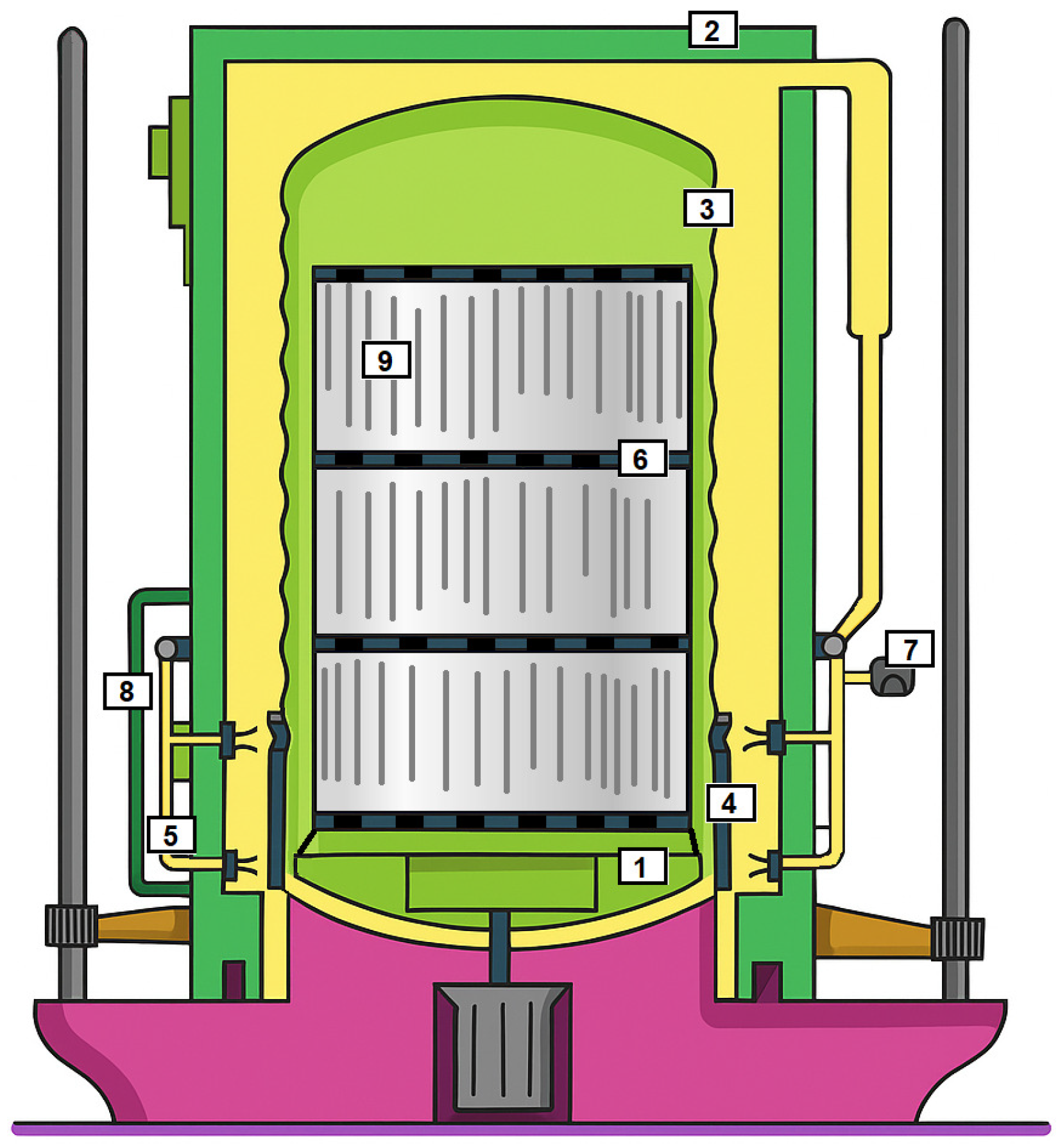
Figure 1. Scheme of bell furnace. Legend: (1) stand, (2) heating cap, (3) muffle with pads, (4) catalytic pads in combustion zone, (5) burners, (6) convection rings, (7) fuel supply control, (8) recuperative oxidizer and fuel system, and (9) steel coil.
Metals 15 00932 g001
Figure 2. Typical batch annealing cycle (temperature vs. time).
Metals 15 00932 g002
Figure 3. Evolution of microstructure (grain growth) in a rolled steel sheet during annealing at different temperatures (qualitative visualization only, not analyzed quantitatively in this study).
Metals 15 00932 g003
Figure 4. Measurement system used during experimental annealing.
Metals 15 00932 g004
Figure 5. Electric furnace with a control system: (a) electrical switchboard with an industrial computer (Quad core-Intel Atom E3940 1.60 GHz, 8 GB SDRAM B&R 5PPC2200.AL18-00; B&R Industrial Automation GmbH, Eggelsberg, Austria), I/Os and communication module; (b) front wall of the switchboard with a display touch panel (18.5″ Full HD TFT B&R 5AP1130.185C-000; B&R Industrial Automation GmbH, Eggelsberg, Austria); (c) experimental electric furnace.
Metals 15 00932 g005
Figure 6. Hardware configuration of the control system of an electric furnace.
Metals 15 00932 g006
Figure 7. The scheme of coil grid parameters.
Metals 15 00932 g007
Figure 8. Placement of thermocouples mapped onto the 2D grid.
Metals 15 00932 g008
Figure 9. Workflow of the proposed approach: from experimental data acquisition to ML model training and evaluation.
Metals 15 00932 g009
Figure 10. Example of input observation as measured surface temperatures.
Metals 15 00932 g010
Figure 11. Measured and simulated temperature T 2 by FDM and SVR (experiment #2): (a) SVR, linear kernel; (b) Gaussian kernel; (c) polynomial kernel.
Metals 15 00932 g011
Figure 12. Measured and simulated temperature T 2 by FDM and SVR (experiment #4): (a) SVR, linear kernel; (b) Gaussian kernel; (c) polynomial kernel.
Metals 15 00932 g012
Figure 13. Measured and simulated temperature T 2 using FDM and NN (experiment #2).
Metals 15 00932 g013
Figure 14. Measured and simulated temperature T 2 using FDM and NN (experiment #4).
Metals 15 00932 g014
Figure 15. Measured and simulated temperature T 2 using FDM and MARS (experiment #2): (a) MARS, piecewise-linear; (b) MARS, piecewise-cubic.
Metals 15 00932 g015
Figure 16. Measured and simulated temperature T 2 using FDM and SVR (experiment #4): (a) MARS, piecewise-linear; (b) MARS, piecewise-cubic.
Metals 15 00932 g016
Figure 17. Measured and simulated temperature T 2 using FDM and k-NN (experiment #2).
Metals 15 00932 g017
Figure 18. Measured and simulated temperature T 2 using FDM and k-NN (experiment #4).
Metals 15 00932 g018
Figure 19. Measured and simulated temperature T 2 using FDM and RF (experiment #2).
Metals 15 00932 g019
Figure 20. Measured and simulated temperature T 2 using FDM and RF (experiment #4).
Metals 15 00932 g020
Figure 21. Arrangement of thermocouples on a stack of four steel coils during the annealing process.
Metals 15 00932 g021
Figure 22. Measured and simulated temperature T 11 using FDM and SVR (operational experiment #1): (a) SVR, linear kernel; (b) SVR, Gaussian kernel; (c) SVR, polynomial kernel.
Metals 15 00932 g022
Figure 23. Measured and simulated temperature T 11 using FDM and NN (operational experiment #1).
Metals 15 00932 g023
Figure 24. Measured and simulated temperature T 11 using FDM and MARS (operational experiment #1): (a) MARS, piecewise-linear; (b) MARS, piecewise-cubic.
Metals 15 00932 g024
Figure 25. Measured and simulated temperature T 11 using FDM, k-NN, and RF (operational experiment #1): (a) k-NN; (b) RF.
Metals 15 00932 g025
Figure 26. Measured and simulated temperature T 2 using FDM and SVR (operational experiment #2): (a) SVR, linear kernel; (b) SVR, Gaussian kernel; (c) SVR, polynomial kernel.
Metals 15 00932 g026
Figure 27. Measured and simulated temperature T 2 using FDM, k-NN, and RF (operational experiment #2): (a) k-NN; (b) RF.
Metals 15 00932 g027
Figure 28. Graphic comparison of the performance index of prediction methods when simulating the internal coil temperature.
Metals 15 00932 g028
Table 1. Boundary conditions and thermophysical properties of the FDM model.
Condition/PropertyDescription/Value
Initial conditionUniform initial temperature T 0
across the domain
Radial outer boundary ( r = R )Dirichlet: measured surface temperature
from thermocouples
Axial boundaries ( z = 0 and z = H )Neumann: insulated boundary ( T z = 0 ) or
measured temperature if available
Thermal conductivity λ 50–80  W m 1 K 1 (20–700 °C)
Density ρ 7800–7850  kg m 3
Specific heat c p 460–600  J kg 1 K 1 (20–700 °C)
Thermal diffusivity α Calculated as α = λ / ( ρ c p )
Table 2. Performance of FDM and ML methods in temperature prediction on test data (experiment #2).
TemperatureMethod r yY r yY 2 MSEMAPE (%)RMSERRMSE (%)PIMax. Deviation (°C)
T 2 FDM0.99770.9953540.44615.033023.24754.70072.353151.4602
SVR (linear kernel)0.99940.9987138.04147.362611.74912.37571.188225.9277
SVR (Gaussian kernel)0.98610.97242767.961622.489752.611410.63825.3564126.5662
SVR (polynomial kernel)0.99770.99541864.674939.340643.18198.73164.370895.0755
Feed-forward NN0.99910.998397.81523.06659.89022.05001.025527.3036
MARS (piecewise-linear)0.99970.999465.77321.82198.11011.63990.820121.2783
MARS (piecewise-cubic)0.99970.999467.20751.96378.19801.65770.829021.6922
k-NN regression0.99920.9984109.86723.587710.48182.11951.060232.7000
RF0.99970.999437.84362.34026.15171.24390.622023.3970
T 3 FDM0.99950.9990170.06993.865413.04112.65411.327426.9984
SVR (linear kernel)0.99990.9998392.390511.751519.80884.03152.015827.1880
SVR (Gaussian kernel)0.99570.99131199.445914.714834.63307.04853.531966.1461
SVR (polynomial kernel)0.99650.99293601.143257.879260.009512.21316.1174146.4095
Feed-forward NN0.99960.999157.35742.42607.57351.54140.770818.3408
MARS (piecewise-linear)0.99990.999818.13662.00054.25870.86670.433415.5551
MARS (piecewise-cubic)0.99990.999720.16402.46944.49040.91390.45708.7338
k-NN regression1.00000.99995.94350.95532.43790.49620.24818.8200
RF0.99990.999913.24930.95933.64000.74080.370412.4364
T 4 FDM0.99990.999758.02732.31717.61761.56680.783413.8095
SVR (linear kernel)0.99940.9989148.02236.051912.16642.50241.251624.4570
SVR (Gaussian kernel)0.98320.96673521.334927.676259.340812.20546.1543136.3094
SVR (polynomial kernel)0.98730.974710,211.8079101.8807101.053520.784910.4590232.3988
Feed-forward NN0.99950.999162.06963.56657.87841.62050.810420.4360
MARS (piecewise-linear)0.99990.999818.13662.00054.25870.86670.433415.5551
MARS (piecewise-cubic)1.00000.999910.44901.62683.23250.66490.332411.4345
k-NN regression0.99990.999815.87171.00353.98390.81940.409713.6000
RF1.00000.99995.39100.76552.32180.47760.23889.7072
Table 3. Performance of FDM and ML methods in temperature prediction on test data (experiment #4).
TemperatureMethod r yY r yY 2 MSEMAPE (%)RMSERRMSE (%)PIMax. Deviation (°C)
T 2 FDM0.99890.9977294.95764.469017.17433.81331.907735.8958
SVR (linear kernel)0.99980.9996574.172213.139523.96195.32042.660532.5186
SVR (Gaussian kernel)0.45830.210154,047.2024140.2450232.480551.619035.3957319.8229
SVR (polynomial kernel)0.98190.964129,834.811874.6854172.727638.351719.3509288.4810
Feed-forward NN0.99680.99351539.802619.035139.24038.71284.363573.9665
MARS (piecewise-linear)0.99980.9995107.77843.036510.38162.30511.152729.2249
MARS (piecewise-cubic)0.99970.9994116.64173.123910.80012.39801.199227.8945
k-NN regression0.99830.9966407.94376.756720.19764.48462.244255.2871
RF0.99480.98971279.22048.642835.76627.94143.9810108.9974
T 3 FDM0.99680.9937763.29086.917227.62776.00633.007960.6107
SVR (linear kernel)0.99920.99841709.891619.414541.35088.98984.496762.6530
SVR (Gaussian kernel)0.53400.285256,215.3635120.7524237.097851.545633.6021304.7536
SVR (polynomial kernel)0.97750.9555131,518.5861249.6136362.654978.842039.8697612.8103
Feed-forward NN0.99550.9909754.17947.514027.46235.97042.992073.8377
MARS (piecewise-linear)0.99900.9980180.08903.127013.41972.91751.459541.2451
MARS (piecewise-cubic)0.99870.9975222.19363.037414.90623.24061.621340.1436
k-NN regression0.99720.9944772.41198.575727.79236.04213.025371.6013
RF0.99390.98781237.61498.622535.17987.64823.8358105.7638
T 4 FDM0.99930.9986315.44784.404117.76093.90191.951631.4712
SVR (linear kernel)0.99980.99961090.549112.481033.02357.25503.627843.3134
SVR (Gaussian kernel)0.40970.167962,362.6146148.8183249.725154.862338.9173316.9154
SVR (polynomial kernel)0.95050.903555,356.7333118.8545235.280151.688026.5003796.2979
Feed-forward NN0.98050.96135101.220172.572671.422815.69097.9229183.1845
MARS (piecewise-linear)0.99960.9993129.34364.336911.37292.49851.249524.3075
MARS (piecewise-cubic)0.99960.9993129.94954.384711.39952.50441.252425.3766
k-NN regression0.99700.9941671.00977.579125.90395.69082.849761.5594
RF0.99350.98711249.50637.106135.34847.76573.8954109.3951
Table 6. Comparison of the performance index (PI) of prediction methods when simulating the internal temperature of a coil based on unknown data.
ScenarioFDMSVR
Linear Kernel
SVR
Gaussian Kernel
SVR
Polynomial Kernel
NNMARS
Piecewise Linear
MARS
Piecewise Cubic
k-NNRF
Laboratory exp. #2 (Temp. T2)2.35311.18825.35644.37081.02550.82010.82901.06020.6220
Laboratory exp. #2 (Temp. T3)1.32742.01583.53196.11740.77080.43340.45700.24810.3704
Laboratory exp. #2 (Temp. T4)0.78341.25166.154310.45900.81040.43340.33240.40970.2388
Laboratory exp. #4 (Temp. T2)1.90772.660535.395719.35094.36351.15271.19922.24423.9810
Laboratory exp. #4 (Temp. T3)3.00794.496733.602139.86972.99201.45951.62133.02533.8358
Laboratory exp. #4 (Temp. T4)1.95163.627838.917326.50037.92291.24951.25242.84973.8954
Operational exp. #1 (Temp. T11)2.31823.61996.18241572.74735.68230.99240.94871.29991.0922
Operational exp. #2 (Temp. T2)2.28335.40093.347021.35255.17891.40201.56960.97610.9018
Operational exp. #2 (Temp. T8)1.03454.62202.98557.534921.99851.47931.71750.93400.9053
Table 7. Comparison of temperature prediction models in steel coil annealing.
ModelApproachPrediction AccuracyNotesReference
Finite Difference
Model (FDM)
Physics-based
(heat conduction)
Max deviation: 11.2 °C,
RMSE: 5.8 °C (test data)
Robust, requires material properties
and boundary conditions
This study
Multivariate Adaptive
Regression Splines (MARS)
Data-driven (ML)Max deviation: 8.9 °C,
RMSE: 4.7 °C (test data)
Good generalization, interpretable
basis functions
This study
Random Forest (RF)Data-driven (ML)Max deviation: 9.3 °C,
RMSE: 5.1 °C (test data)
Robust to noise and overfitting,
handles large datasets
This study
Physics-informed Neural
Networks (PINNs)
Hybrid
(Physics + ML)
MAE: 7.2 °C
(additive manufacturing data)
Combines PDE constraints with
data-driven learning
[13]
Analytical thermal model for
bell-type annealing
Physics-based
(analytical)
Relative error: <0.5% at cold spot,
<5% at hot spot
Simplified analytical formulation[12]
Neural Network model for
annealing furnaces
Data-driven (ML)RMSE: 8.7 °CTrained on noisy industrial data[18]
Finite Difference Model
(hydrogen annealing)
Physics-based (FDM)Max deviation: 12.4 °C
(core temperatures)
Calibrated with industrial data[10]
Disclaimer/Publisher’s Note: The statements, opinions and data contained in all publications are solely those of the individual author(s) and contributor(s) and not of MDPI and/or the editor(s). MDPI and/or the editor(s) disclaim responsibility for any injury to people or property resulting from any ideas, methods, instructions or products referred to in the content.