
Comparison of Fatigue Property Estimation Methods with Physical Test Data


Abstract
1. Introduction
2. Empirical Methods for Determining Material Fatigue Parameters
2.1. FPCM—Four-Point Correlation Method
2.2. USM—Universal Slope Method
2.3. MUSM—Modified Universal Slope Method
2.4. UMLM—Uniform Material Law Method
2.5. MFPCM—Modified Four-Point Correlation Method
2.6. MM—Median Method
2.7. RF—Roessle–Fatemi Method
2.8. Physical Test Data
- Tension strength ()—The maximum stress a material can withstand while being subject to uniaxial tension load.
- Elongation at break ()—The measure of a material’s expandability, indicating how much it can stretch before breaking.
- Reduction of the cross-section area ()—The decrease in cross-sectional area at the point of fracture, reflecting the material’s ability to undergo plastic deformation before failure. This value can be obtained only from a test or the literature.
- Young modulus ()—The measure of a material’s stiffness, defined as the ratio of tension stress to tension strain in the linear elastic region.
- Hardness ()—The measure of material resistance to surface deflection.
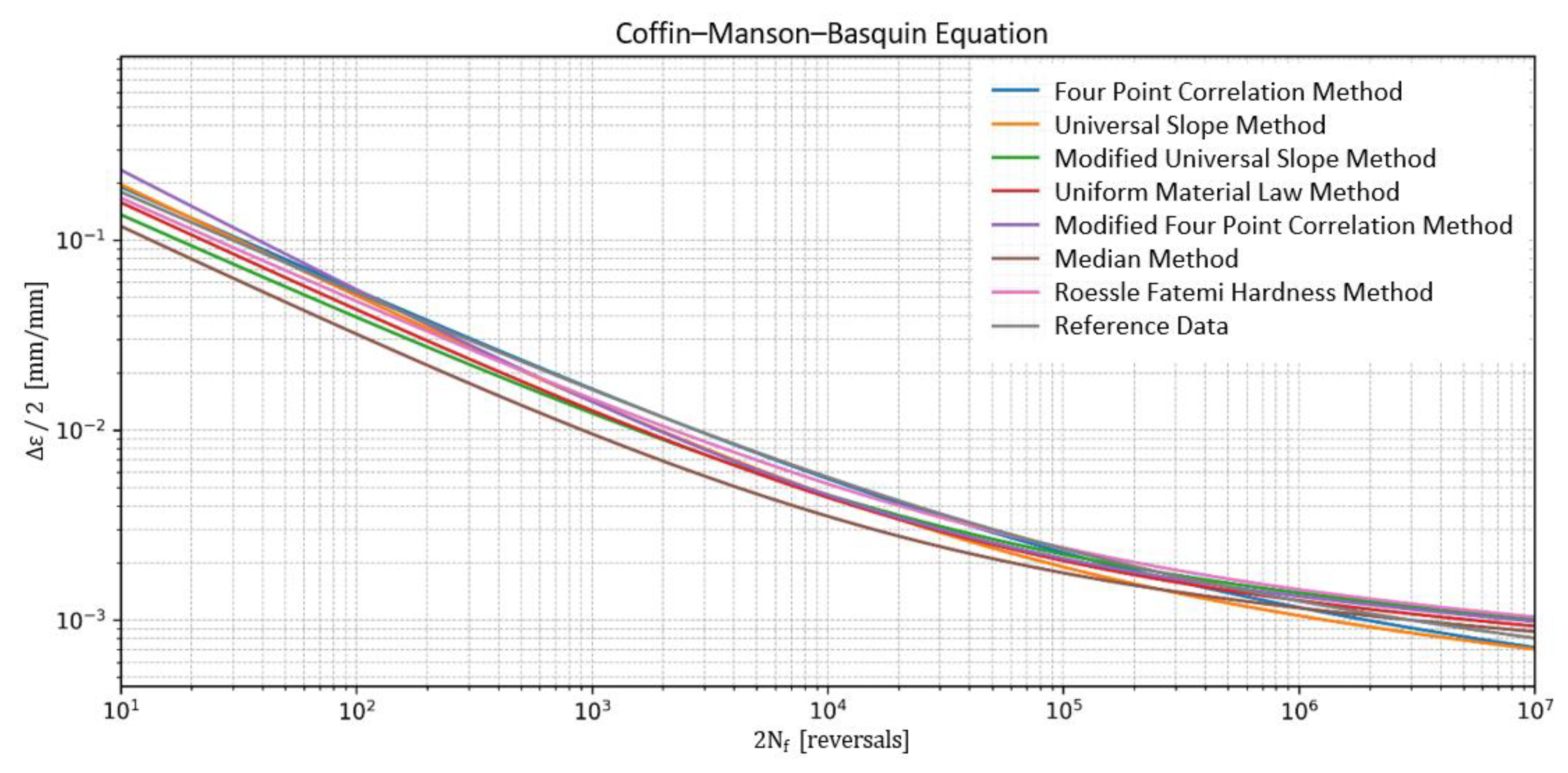
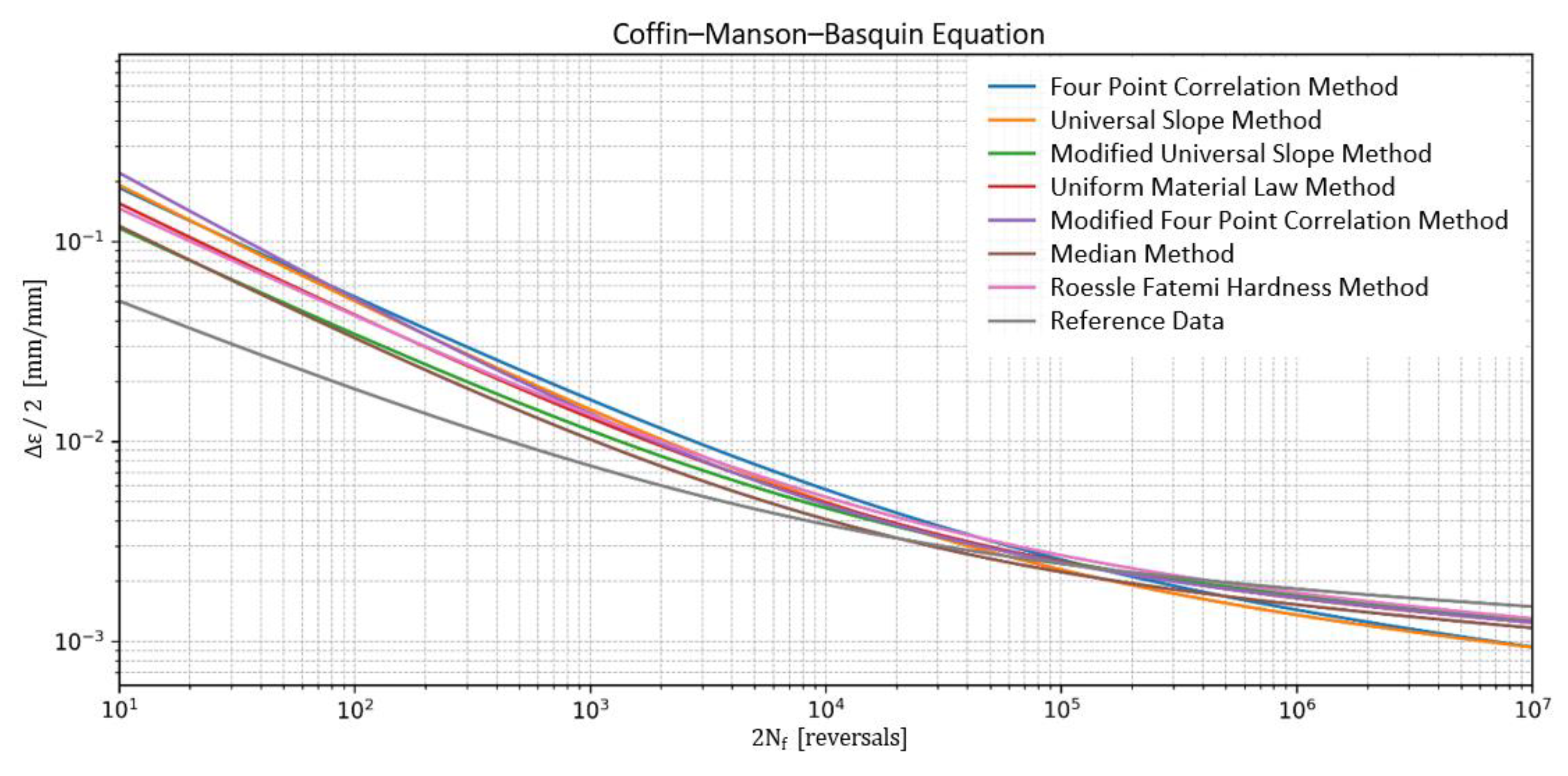
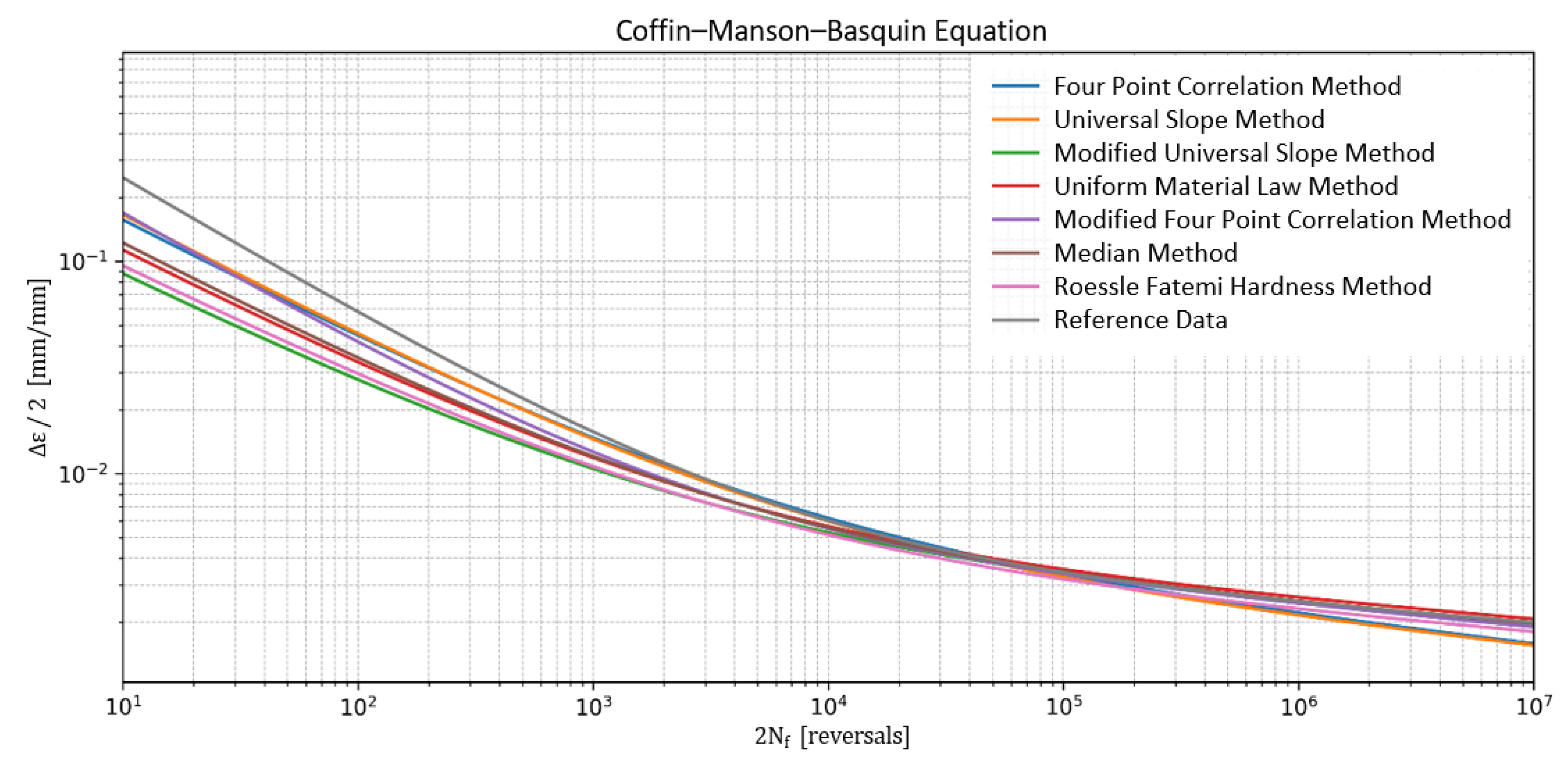
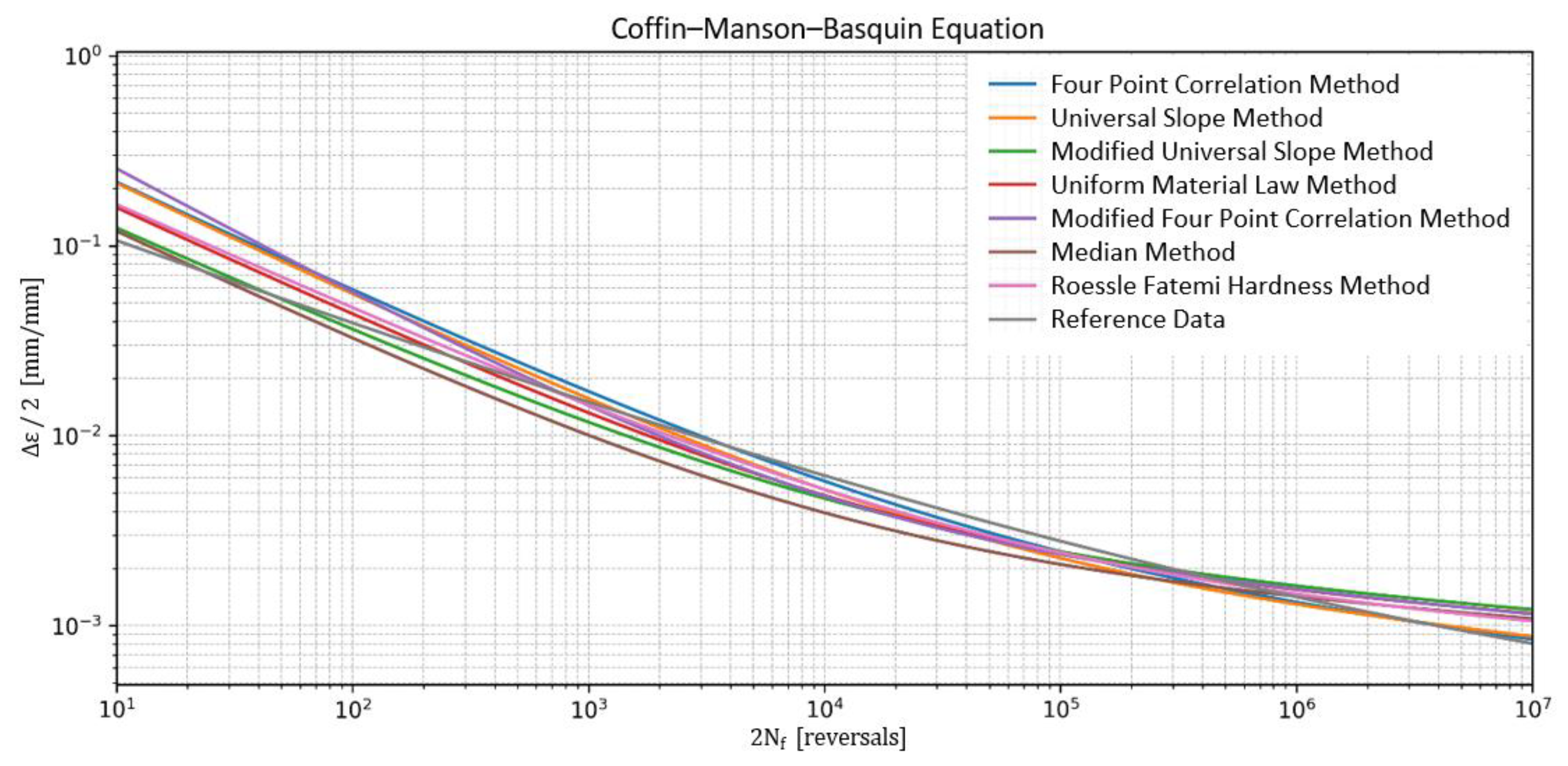
2.9. Validation of Accuracy of the Fatigue Parameter Estimation Methods
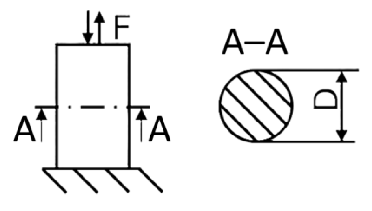
3. Load Case Description
4. Analysis and Discussion

| Method | [MPa] | b [-] | [-] | c [-] | RMSLE | Emax |
|---|---|---|---|---|---|---|
| Four-point correlation method | 1151.60 | −0.1338 | 0.6760 | −0.5581 | 0.25 | 0.70 |
| Universal slope method | 950.90 | −0.1200 | 0.7677 | −0.6000 | 0.53 | 0.84 |
| Modified universal slope method | 859.34 | −0.0900 | 0.4831 | −0.5600 | 0.89 | 2.65 |
| Uniform material law method | 750.00 | −0.0870 | 0.5900 | −0.5800 | 0.59 | 1.81 |
| Modified four-point correlation method | 1010.83 | −0.1005 | 1.0217 | −0.6466 | 0.71 | 2.17 |
| Median method | 750.00 | −0.0900 | 0.4500 | −0.5900 | 0.91 | 1.19 |
| Roessle–Fatemi method | 866.75 | −0.0900 | 0.5941 | −0.5600 | 0.86 | 2.77 |
| Reference data | 1000.00 | −0.1180 | 0.6190 | −0.5460 | 0.00 | 0.00 |

| Method | [MPa] | b [-] | [-] | c [-] | RMSLE | Emax |
|---|---|---|---|---|---|---|
| Four-point correlation method | 1672.02 | −0.1405 | 0.8449 | −0.5914 | 1.26 | 2.50 |
| Universal slope method | 1272.30 | −0.1200 | 0.8472 | −0.6000 | 1.26 | 2.49 |
| Modified universal slope method | 1094.90 | −0.0900 | 0.4247 | −0.5600 | 0.50 | 0.94 |
| Uniform material law method | 1003.50 | −0.0870 | 0.5773 | −0.5800 | 0.72 | 1.41 |
| Modified four-point correlation method | 1474.46 | −0.1108 | 1.2040 | −0.6775 | 0.99 | 2.20 |
| Median method | 1003.50 | −0.0900 | 0.4500 | −0.5900 | 0.93 | 1.39 |
| Roessle–Fatemi method | 1117.50 | −0.0900 | 0.4897 | −0.5600 | 0.50 | 1.19 |
| Reference data | 845.00 | −0.0750 | 0.2350 | −0.4600 | 0.00 | 0.00 |
| Method | [MPa] | b [-] | [-] | c [-] | RMSLE | Emax |
|---|---|---|---|---|---|---|
| Four-point correlation method | 1483.86 | −0.1317 | 0.6669 | −0.5672 | 1.75 | 2.92 |
| Universal slope method | 1257.09 | −0.1200 | 0.7431 | −0.6000 | 1.73 | 3.22 |
| Modified universal slope method | 1079.62 | −0.0900 | 0.4079 | −0.5600 | 1.05 | 1.78 |
| Uniform material law method | 991.50 | −0.0870 | 0.5744 | −0.5800 | 1.33 | 2.27 |
| Modified four-point correlation method | 1300.57 | −0.1027 | 0.9676 | −0.6523 | 1.45 | 2.75 |
| Median method | 991.50 | −0.0900 | 0.4500 | −0.5900 | 1.21 | 2.41 |
| Roessle–Fatemi method | 1083.50 | −0.0900 | 0.5155 | −0.5600 | 1.30 | 2.19 |
| Reference data | 799.00 | −0.0620 | 0.1440 | −0.4860 | 0.00 | 0.00 |

| Method | [MPa] | b [-] | [-] | c [-] | RMSLE | Emax |
|---|---|---|---|---|---|---|
| Four-point correlation method | 2037.30 | −0.1267 | 0.6375 | −0.5863 | 1.04 | 2.35 |
| Universal slope method | 1835.24 | −0.1200 | 0.6846 | −0.6000 | 1.07 | 2.46 |
| Modified universal slope method | 1470.46 | −0.0900 | 0.3208 | −0.5600 | 0.20 | 0.70 |
| Uniform material law method | 1447.50 | −0.0870 | 0.4523 | −0.5800 | 0.39 | 0.61 |
| Modified four-point correlation method | 1779.43 | −0.1037 | 0.8440 | −0.6618 | 0.69 | 1.40 |
| Median method | 1447.50 | −0.0900 | 0.4500 | −0.5900 | 0.38 | 0.88 |
| Roessle–Fatemi method | 1355.50 | −0.0900 | 0.4247 | −0.5600 | 0.56 | 1.37 |
| Reference data | 1087.00 | −0.0680 | 0.3120 | −0.5490 | 0.00 | 0.00 |
| Method | [MPa] | b [-] | [-] | c [-] | RMSLE | Emax |
|---|---|---|---|---|---|---|
| Four-point correlation method | 2306.53 | −0.1219 | 0.5730 | −0.5857 | 0.74 | 1.89 |
| Universal slope method | 2202.28 | −0.1200 | 0.6295 | −0.6000 | 0.78 | 2.05 |
| Modified universal slope method | 1728.33 | −0.0900 | 0.2941 | −0.5600 | 1.10 | 2.24 |
| Uniform material law method | 1737.00 | −0.0870 | 0.4049 | −0.5800 | 0.81 | 1.64 |
| Modified four-point correlation method | 2007.94 | −0.1010 | 0.7340 | −0.6557 | 0.42 | 0.62 |
| Median method | 1737.00 | −0.0900 | 0.4500 | −0.5900 | 0.70 | 1.44 |
| Roessle–Fatemi method | 1580.75 | −0.0900 | 0.3248 | −0.5600 | 1.10 | 2.06 |
| Reference data | 1574.00 | −0.0830 | 1.1090 | −0.6610 | 0.00 | 0.00 |
| Method | [MPa] | b [-] | [-] | c [-] | RMSLE | Emax |
|---|---|---|---|---|---|---|
| Four-point correlation method | 1552.37 | −0.1394 | 0.8111 | −0.5847 | 0.66 | 1.60 |
| Universal slope method | 1198.13 | −0.1200 | 0.8333 | −0.6000 | 0.70 | 1.58 |
| Modified universal slope method | 1041.53 | −0.0900 | 0.4365 | −0.5600 | 1.51 | 5.11 |
| Uniform material law method | 945.00 | −0.0870 | 0.5900 | −0.5800 | 1.36 | 4.75 |
| Modified four-point correlation method | 1367.85 | −0.1089 | 1.1712 | −0.6714 | 1.30 | 3.80 |
| Median method | 945.00 | −0.0900 | 0.4500 | −0.5900 | 1.26 | 4.03 |
| Roessle–Fatemi method | 883.75 | −0.0900 | 0.5867 | −0.5600 | 0.96 | 3.37 |
| Reference data | 1492.00 | −0.1520 | 0.2890 | −0.4540 | 0.00 | 0.00 |
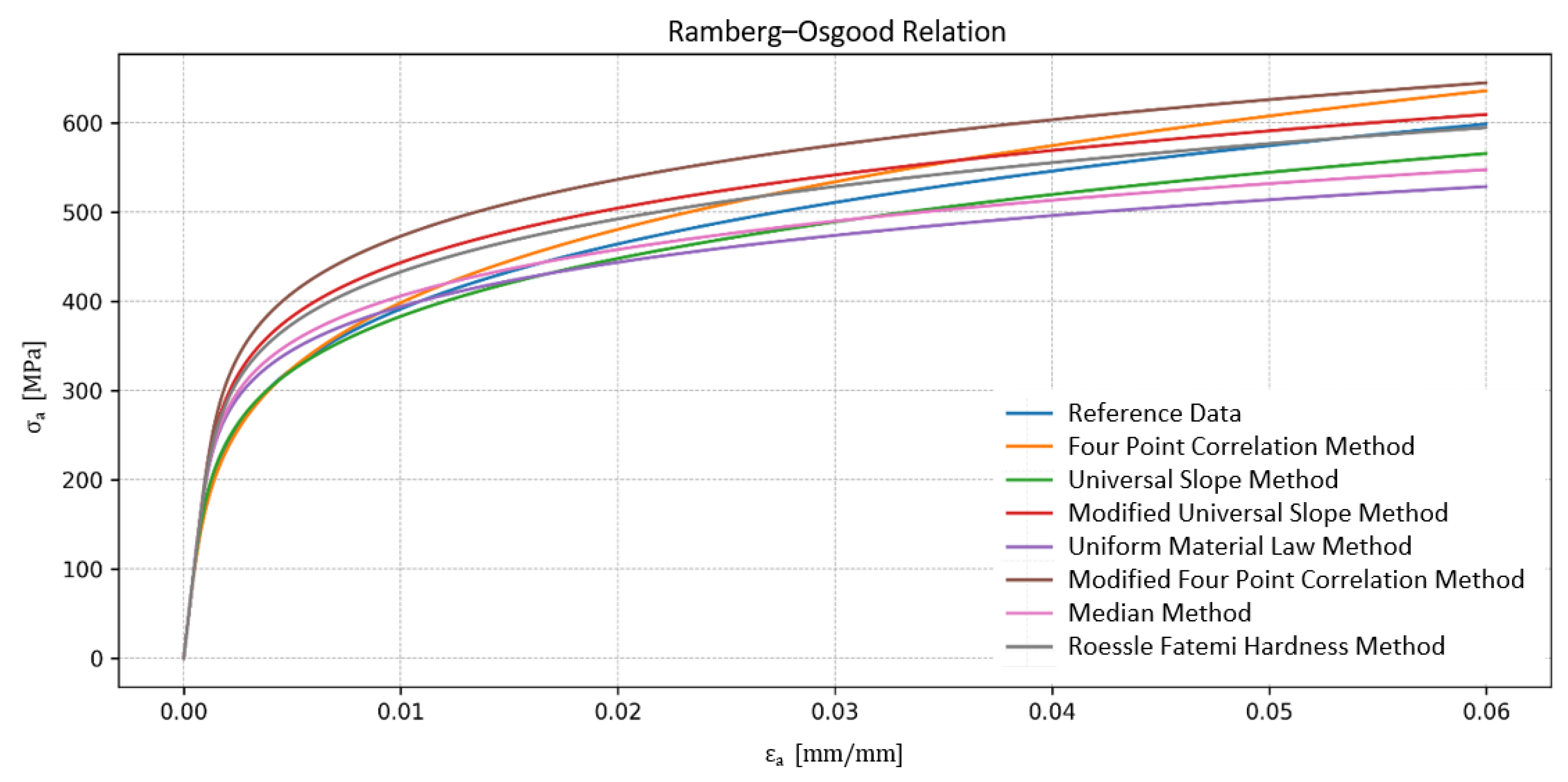
| Method | K’ [MPa] | n’ [-] | L [-] |
|---|---|---|---|
| Four-point correlation method | 1264.98 | 0.2398 | 4.48 |
| Universal slope method | 1002.53 | 0.2000 | 4.21 |
| Modified universal slope method | 965.93 | 0.1607 | 8.48 |
| Uniform material law method | 811.77 | 0.1500 | 7.59 |
| Modified four-point correlation method | 1007.46 | 0.1555 | 15.03 |
| Median method | 847.15 | 0.1525 | 5.34 |
| Roessle–Fatemi method | 942.41 | 0.1607 | 6.29 |
| Reference data | 1118.00 | 0.2180 | 0.00 |
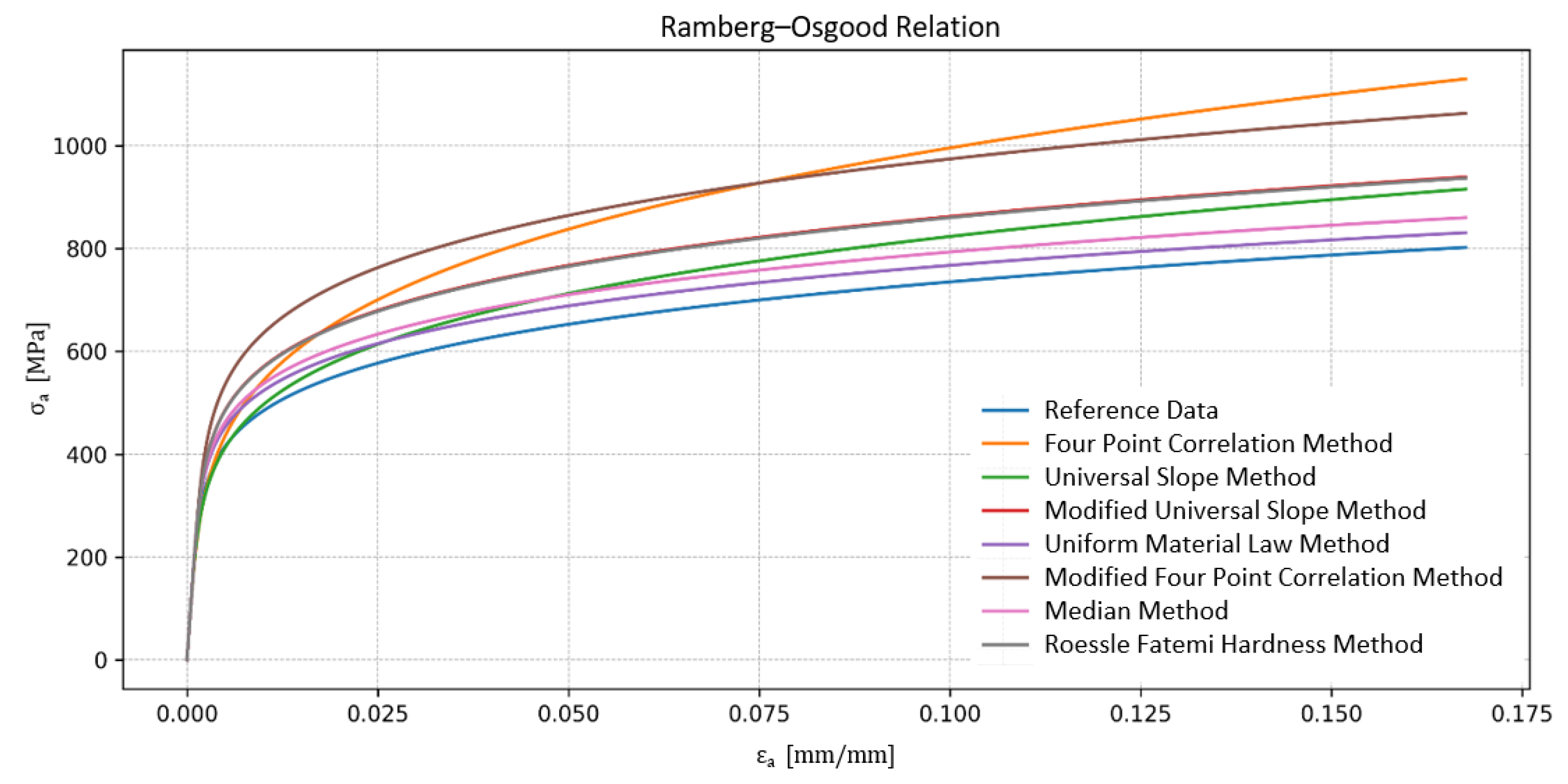
| Method | K’ [MPa] | n’ [-] | L [-] |
|---|---|---|---|
| Four-point correlation method | 1740.34 | 0.2376 | 71.96 |
| Universal slope method | 1315.21 | 0.2000 | 23.92 |
| Modified universal slope method | 1256.47 | 0.1607 | 40.27 |
| Uniform material law method | 1089.71 | 0.1500 | 12.22 |
| Modified four-point correlation method | 1430.38 | 0.1635 | 74.79 |
| Median method | 1133.49 | 0.1525 | 19.89 |
| Roessle–Fatemi method | 1253.36 | 0.1607 | 39.61 |
| Reference data | 1081.00 | 0.1650 | 0.00 |
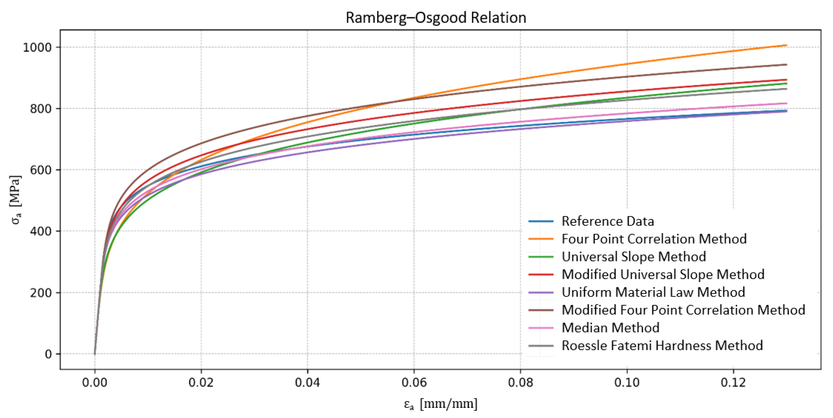
| Method | K’ [MPa] | n’ [-] | L [-] |
|---|---|---|---|
| Four-point correlation method | 1630.23 | 0.2322 | 29.75 |
| Universal slope method | 1334.02 | 0.2000 | 11.18 |
| Modified universal slope method | 1246.98 | 0.1607 | 17.69 |
| Uniform material law method | 1077.48 | 0.1500 | 5.95 |
| Modified four-point correlation method | 1307.34 | 0.1575 | 29.85 |
| Median method | 1119.93 | 0.1525 | 3.32 |
| Roessle–Fatemi method | 1205.24 | 0.1607 | 11.00 |
| Reference data | 1038.00 | 0.1300 | 0.00 |
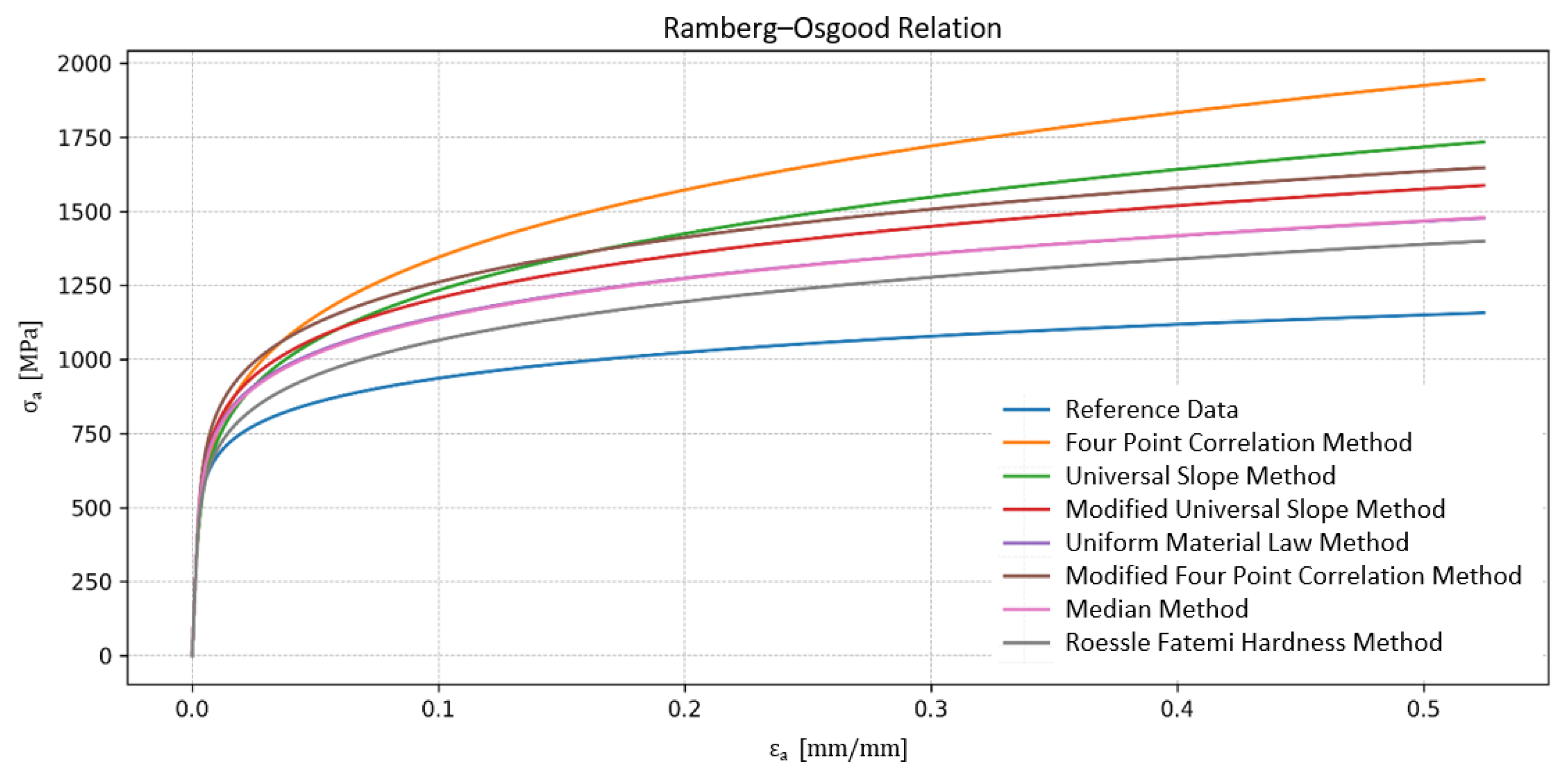
| Method | K’ [MPa] | n’ [-] | L [-] |
|---|---|---|---|
| Four-point correlation method | 2245.43 | 0.2161 | 300.77 |
| Universal slope method | 1979.75 | 0.2000 | 219.58 |
| Modified universal slope method | 1765.24 | 0.1607 | 183.18 |
| Uniform material law method | 1630.42 | 0.1500 | 138.80 |
| Modified four-point correlation method | 1827.37 | 0.1567 | 215.25 |
| Median method | 1635.00 | 0.1525 | 137.61 |
| Roessle–Fatemi method | 1555.48 | 0.1607 | 93.82 |
| Reference data | 1256.00 | 0.1250 | 0.00 |
| Method | K’ [MPa] | n’ [-] | L [-] |
|---|---|---|---|
| Four-point correlation method | 2590.04 | 0.2082 | 268.37 |
| Universal slope method | 2415.85 | 0.2000 | 221.85 |
| Modified universal slope method | 2104.04 | 0.1607 | 169.98 |
| Uniform material law method | 1989.26 | 0.1500 | 142.48 |
| Modified four-point correlation method | 2105.87 | 0.1540 | 181.10 |
| Median method | 1962.00 | 0.1525 | 128.27 |
| Roessle–Fatemi method | 1893.87 | 0.1607 | 91.20 |
| Reference data | 1543.00 | 0.1250 | 0.00 |
| Method | K’ [MPa] | n’ [-] | L [-] |
|---|---|---|---|
| Four-point correlation method | 1631.81 | 0.2383 | 8.41 |
| Universal slope method | 1242.65 | 0.2000 | 9.46 |
| Modified universal slope method | 1189.94 | 0.1607 | 12.83 |
| Uniform material law method | 1022.83 | 0.1500 | 12.02 |
| Modified four-point correlation method | 1333.24 | 0.1622 | 21.72 |
| Median method | 1067.41 | 0.1525 | 11.30 |
| Roessle–Fatemi method | 962.83 | 0.1607 | 16.99 |
| Reference data | 2242.00 | 0.3320 | 0.00 |
| Method | Life [Cycles] | |||||
|---|---|---|---|---|---|---|
| Unalloyed Steel | Low-Alloy Steel | High-Alloy Steel | ||||
| SB46 | S35C | RHW 38 | 8Mn6 | SUH 660-B | SUH 310-B | |
| Four-point correlation method | 3.99 | 5.98 | 9.83 | 12.73 | 6.88 | 7.16 |
| Universal slope method | 2.50 | 4.47 | 6.74 | 10.42 | 5.93 | 5.19 |
| Modified universal slope method | 3.54 | 4.80 | 9.11 | 11.35 | 5.08 | 6.28 |
| Uniform material law method | 2.64 | 4.50 | 8.59 | 13.99 | 6.86 | 5.60 |
| Modified four-point correlation method | 4.00 | 6.30 | 10.94 | 14.19 | 6.49 | 7.82 |
| Median method | 1.54 | 2.73 | 5.23 | 10.79 | 5.98 | 3.30 |
| Roessle–Fatemi method | 4.76 | 6.14 | 12.02 | 9.78 | 3.63 | 5.18 |
| Reference data | 4.21 | 5.02 | 5.16 | 7.60 | 6.38 | 6.35 |
| Method | Error in Life [%] | |||||
|---|---|---|---|---|---|---|
| Unalloyed Steel | Low-Alloy Steel | High-Alloy Steel | ||||
| SB46 | S35C | RHW 38 | 8Mn6 | SUH 660-B | SUH 310-B | |
| Four-point correlation method | 3.70 | 10.81 | 39.21 | 25.41 | 4.07 | 6.49 |
| Universal slope method | 36.24 | 7.18 | 16.17 | 15.52 | 3.93 | 10.91 |
| Modified universal slope method | 11.91 | 2.80 | 34.55 | 19.75 | 12.30 | 0.56 |
| Uniform material law method | 32.41 | 6.83 | 31.00 | 30.06 | 3.94 | 6.80 |
| Modified four-point correlation method | 3.52 | 14.05 | 45.70 | 30.73 | 0.99 | 11.25 |
| Median method | 69.75 | 37.88 | 0.77 | 17.24 | 3.48 | 35.46 |
| Roessle–Fatemi method | 8.59 | 12.41 | 51.43 | 12.39 | 30.36 | 11.01 |
| Reference data | 0.00 | 0.00 | 0.00 | 0.00 | 0.00 | 0.00 |
5. Conclusions
| Material Type | Best Estimation Method (Life Prediction) | Notes |
|---|---|---|
| Unalloyed Steel | MUSM (for S35C), FPCM (for SB46) | Good RMSLE and low Emax; reliable for low-to-moderate cycle fatigue |
| Low-Alloy Steel | MM (RHW 38), RF (8Mn6) | MM highly accurate in some cases, but inconsistent |
| High-Alloy Steel | MFPCM (SUH 660-B), MUSM (SUH 310-B) | Strong correlation despite poor cyclic stress–strain curve fit |
6. Future Directions
Author Contributions
Funding
Data Availability Statement
Conflicts of Interest
Abbreviations and Symbols
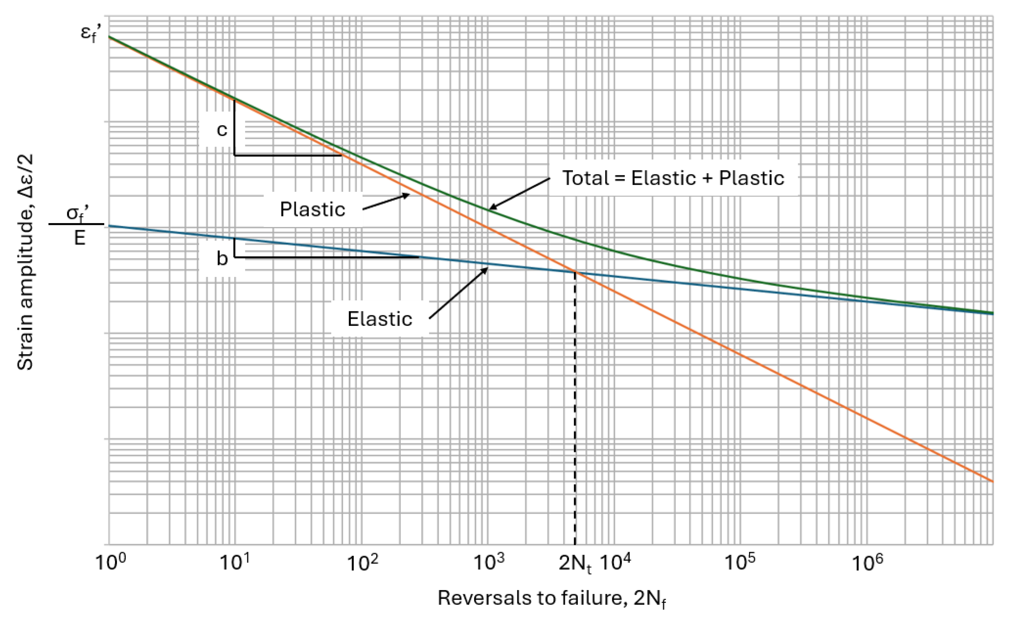
| 2Nf | Reversals to failure |
| b | Fatigue strength exponent |
| c | Fatigue ductility exponent |
| ∆ε | Total strain range |
| ∆εp | Plastic strain range |
| E | Young’s modulus |
| Emax | Logarithmic maximum error |
| E% | Logarithmic percent error |
| ε | Strain |
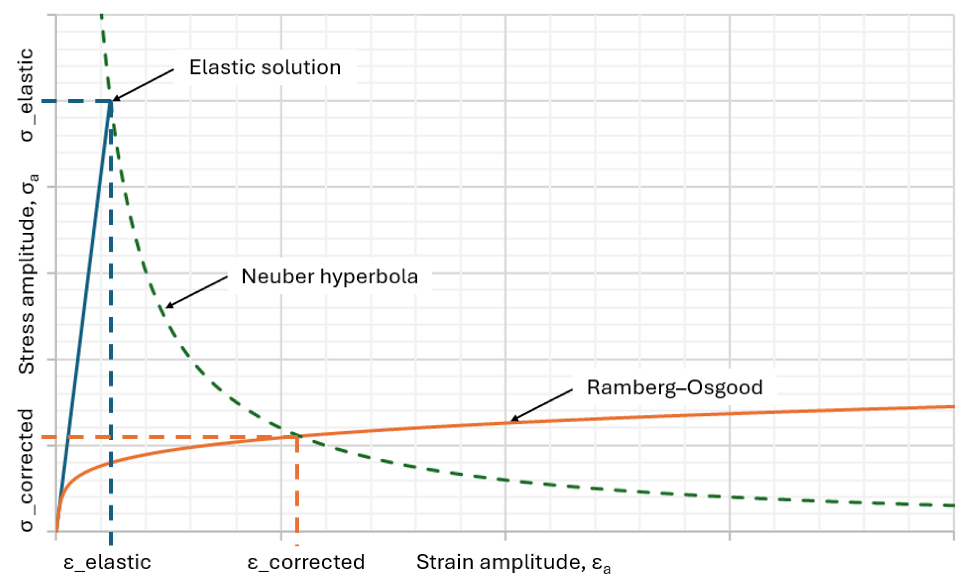
| εa | Strain amplitude |
| εf | Elongation at break |
| Fatigue ductility coefficient | |
| HB | Brinell hardness |
| K’ | Cyclic strength coefficient |
| Kt | Stress concentration factor |
| L | Integral of squared differences |
| n’ | Cyclic strain hardening exponent |
| ψ | Material dependent factor |
| RA | Reduction in area |
| RMSLE | Root mean square logarithmic error |
| σ | Stress |
| σa | Stress amplitude |
| σf | True fracture strength |
| Fatigue strength coefficient | |
| σm | Mean stress |
| σY | Yield strength |
| σUTS | Ultimate tension strength |
| Z | Ductility |
References
- Campbell, F.C. Fatigue and Fracture: Understanding the Basics; ASM International: Materials Park, OH, USA, 2012; ISBN 978-l-61503-976-0. [Google Scholar]
- Tridello, A.; Boursier Niutta, C.; Rossetto, M.; Berto, F.; Paolino, D.S. Fatigue Design Curves for Industrial Applications: A Review. Fatigue Fract. Eng. Mater. Struct. 2025, 48, ffe.14545. [Google Scholar] [CrossRef]
- Fischer, A.; Izmailov, A.F.; Solodov, M.V. The Levenberg–Marquardt Method: An Overview of Modern Convergence Theories and More. Comput. Optim. Appl. 2024, 89, 33–67. [Google Scholar] [CrossRef]
- Gomes, V.M.G.; Souto, C.D.S.; Correia, J.A.F.O.; De Jesus, A.M.P. Monotonic and Fatigue Behaviour of the 51CrV4 Steel with Application in Leaf Springs of Railway Rolling Stock. Metals 2024, 14, 266. [Google Scholar] [CrossRef]
- Ramírez-Acevedo, D.; Ambriz, R.R.; García, C.J.; Gómora, C.M.; Jaramillo, D. Fatigue Damage Assessment in AL6XN Stainless Steel Based on the Strain-Hardening Exponent n-Value. Metals 2025, 15, 472. [Google Scholar] [CrossRef]
- Lipski, A.; Mroziński, S. Approximate Determination of a Strain-Controlled Fatigue Life Curve for Aluminum Alloy Sheets. J. Pol. CIMAC Gdań. Univ. Technol. 2011, 6, 107–118. [Google Scholar]
- Nieslony, A.; Dsoki, C.; Kaufmann, H.; Krug, P. New Method for Evaluation of the Manson–Coffin–Basquin and Ramberg–Osgood Equations with Respect to Compatibility. Int. J. Fatigue 2008, 30, 1967–1977. [Google Scholar] [CrossRef]
- Roark, R.J.; Young, W.C.; Budynas, R.G. Roark’s Formulas for Stress and Strain, 7th ed.; McGraw-Hill: New York, NY, USA, 2002; ISBN 978-0-07-072542-3. [Google Scholar]
- Wollmann, J.; Dolny, A.; Kaszuba, M.; Gronostajski, Z.; Gude, M. Methods for Determination of Low-Cycle Properties from Monotonic Tensile Tests of 1.2344 Steel Applied for Hot Forging Dies. Int. J. Adv. Manuf. Technol. 2019, 102, 3357–3367. [Google Scholar] [CrossRef]
- Harun, M.F.; Mohammad, R.; Othman, N.; Amrin, A.; Chelliapan, S.; Maarop, N. Methods for Estimating the Fatigue Properties of UNS C70600 Copper-Nickel 90/10. Int. J. Mech. Eng. Technol. 2017, 8, 413–422. [Google Scholar]
- Basan, R.; Marohnić, T.; Marković, E. Evaluation of Fatigue Parameters Estimation Methods with Regard to Specific Ranges of Fatigue Lives and Relevant Monotonic Properties. Procedia Struct. Integr. 2022, 42, 655–662. [Google Scholar] [CrossRef]
- Shamsaei, N.; Fatemi, A. Effect of Hardness on Multiaxial Fatigue Behaviour and Some Simple Approximations for Steels. Fatigue Fract. Eng. Mater. Struct. 2009, 32, 631–646. [Google Scholar] [CrossRef]
- Basan, R.; Marohnić, T. A Comprehensive Evaluation of Conventional Methods for Estimation of Fatigue Parameters of Steels from Their Monotonic Properties. Int. J. Fatigue 2024, 183, 108244. [Google Scholar] [CrossRef]
- Park, J.; Song, J. Detailed Evaluation of Methods for Estimation of Fatigue Properties. Int. J. Fatigue 1995, 17, 365–373. [Google Scholar] [CrossRef]
- ISO 6892-1; International Standard. Metallic Materials—Tensile Testing—Part 1: Method of Test at Room Temperature. ISO: Geneva, Switzerland, 2009.
- Colin, J.; Fatemi, A.; Taheri, S. Cyclic Hardening and Fatigue Behavior of Stainless Steel 304L. J. Mater. Sci. 2011, 46, 145–154. [Google Scholar] [CrossRef]
- ISO 12106; International Standard. Metallic Materials—Fatigue Testing—Axial-Strain-Controlled Method. ISO: Geneva, Switzerland, 2017.
- ISO 6506-1; International Standard. Metallic Materials—Brinell Hardness Test—Part 1: Test Method. ISO: Geneva, Switzerland, 2005.
- ISO 18265; International Standard. Metallic Materials—Conversion of Hardness Values. ISO: Geneva, Switzerland, 2013.
- Ince, A.; Glinka, G. A Modification of Morrow and Smith-Watson-Topper Mean Stress Correction Models. Fatigue Fract. Eng. Mater. Struct. 2011, 34, 854–867. [Google Scholar] [CrossRef]
- Böller, C.; Seeger, T. Materials Data for Cyclic Loading; Elsevier Science Publishers: Amsterdam, The Netherlands, 1987; Volumes A–C. [Google Scholar]
- Tao, Z.-Q.; Pan, X.; Zhang, Z.-L.; Chen, H.; Li, L.-X. Multiaxial Fatigue Lifetime Estimation Based on New Equivalent Strain Energy Damage Model under Variable Amplitude Loading. Crystals 2024, 14, 825. [Google Scholar] [CrossRef]
- Batsoulas, N.D.; Giannopoulos, G.I. Cumulative Fatigue Damage of Composite Laminates: Engineering Rule and Life Prediction Aspect. Materials 2023, 16, 3271. [Google Scholar] [CrossRef]
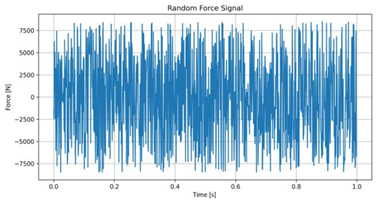
| Unalloyed steel | |
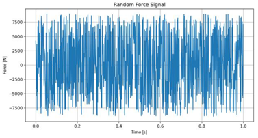 Random load signal for SB46 |  Random load signal for S35C |
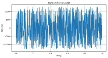
| Low-alloy steel | |
 Random load signal for RHW 38 | 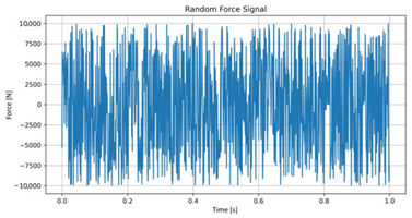 Random load signal for 8Mn6 |
| High-alloy steel | |
 Random load signal for SUH 660-B | 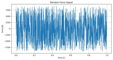 Random load signal for SUH 310-B |
| Material Type | Designation Usual Commercial Designation (e.g., ASTM, SAE, JIS) |
|---|---|
| Unalloyed steel | SB46 |
| S35C | |
| Low-alloy steel | RHW 38 |
| 8Mn6 | |
| High-alloy steel | SUH 660-B |
| SUH 310-B |
| Designation | σUTS [MPa] | σY [MPa] | E [MPa] | A5 [%] | RA [%] | Hardness [HB] |
|---|---|---|---|---|---|---|
| SB46 | 500 | 310 | 210,000 | 30 | 64 | 151 |
| S35C | 669 | 513 | 210,000 | 29 | 70 | 210 |
| RHW 38 | 661 | 517 | 205,000 | 22 | 62 | 202 |
| 8Mn6 | 965 | 862 | 198,000 | 12 | 57 | 266 |
| SUH 660-B | 1158 | 777 | 210,000 | 23 | 52 | 319 |
| SUH 310-B | 630 | 271 | 210,000 | 45 | 69 | 155 |
Disclaimer/Publisher’s Note: The statements, opinions and data contained in all publications are solely those of the individual author(s) and contributor(s) and not of MDPI and/or the editor(s). MDPI and/or the editor(s) disclaim responsibility for any injury to people or property resulting from any ideas, methods, instructions or products referred to in the content. |
© 2025 by the authors. Licensee MDPI, Basel, Switzerland. This article is an open access article distributed under the terms and conditions of the Creative Commons Attribution (CC BY) license (https://creativecommons.org/licenses/by/4.0/).
Share and Cite
Raczek, S.; Niesłony, A.; Kluger, K.; Łukasik, T. Comparison of Fatigue Property Estimation Methods with Physical Test Data. Metals 2025, 15, 780. https://doi.org/10.3390/met15070780
Raczek S, Niesłony A, Kluger K, Łukasik T. Comparison of Fatigue Property Estimation Methods with Physical Test Data. Metals. 2025; 15(7):780. https://doi.org/10.3390/met15070780
Chicago/Turabian StyleRaczek, Sebastian, Adam Niesłony, Krzysztof Kluger, and Tomasz Łukasik. 2025. "Comparison of Fatigue Property Estimation Methods with Physical Test Data" Metals 15, no. 7: 780. https://doi.org/10.3390/met15070780
APA StyleRaczek, S., Niesłony, A., Kluger, K., & Łukasik, T. (2025). Comparison of Fatigue Property Estimation Methods with Physical Test Data. Metals, 15(7), 780. https://doi.org/10.3390/met15070780