Depth-Resolved Elemental Analysis by Glow Discharge Emission Spectroscopy: Practical Aspects—A Review

Abstract

Glow discharge optical emission spectroscopy (GDOES) is a powerful and well-established method of elemental analysis of metals, coatings and surface-modified materials. This review contains essential information needed to establish and successfully run a GDOES laboratory and perform accurate, quantitative GDOES analyses. The basics of the methodology, instrumentation and analytical interpretation of experimental data are presented, and examples of typical depth profiling applications are given. Special attention is paid to application-specific calibrations, their assumptions and prerequisites. The calibration model of GDOES is special; besides the composition of calibration samples, their sputter rates (sputter factors) need to be accounted for. Typical analytical performance of GDOES is discussed (precision, accuracy), as well as the depth quantification in depth-profiling applications. Links to some other methods, complementary to GDOES, are mentioned, including the type and the character of analytical information each method can deliver.

1. Introduction

Glow discharge optical emission spectroscopy (GDOES) has been around for almost 60 years, since its inception in the late 1960s. The invention of the glow discharge spectral source, the Grimm lamp [1], was motivated by an effort to extend and possibly improve analysis of metals by emission spectroscopy, then solely relying on spark excitation. The fact that the initial development of GDOES occurred in an application-oriented laboratory, busy with practical analyses, led to the adoption of the existing analytical procedures and methodology for bulk analysis. Only later was the physics of analytical glow discharges explored [2,3,4], and the methodology for depth-resolved analysis of coatings and surface-modified materials by GDOES was developed [5,6]. The link to bulk analysis remains strong until now, and glow discharge spectroscopy is the only depth profiling technique that can deliver analytical performance as good as that of the best techniques for bulk analysis of metals, alloys and other solid conductive materials. Various modifications of the glow discharge source were proposed and characterized [7,8,9,10], but none are used for routine analyses in commercial instruments. The purpose of this paper is to review the key features of GDOES, describe essential procedures for a successful implementation of GDOES in a materials science laboratory and show what kind of analytical information GDOES can deliver and how to interpret experimental data.

2. The Principle of GDOES, the Grimm-Type Spectral Source

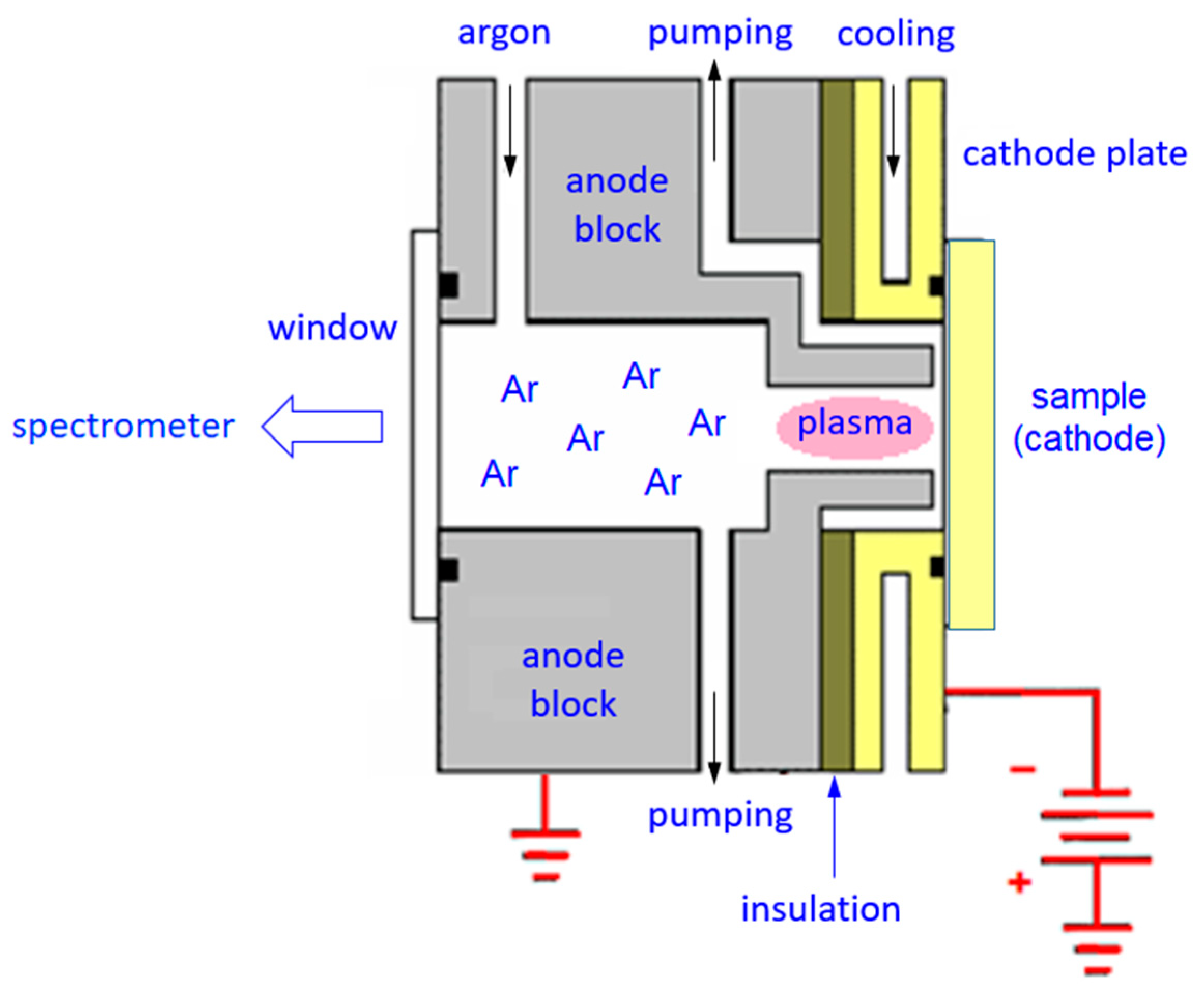
The Grimm-type spectral source is schematically depicted in Figure 1. A flat sample to be analyzed is placed onto the cathode plate, with a circular opening and a sealing o-ring. The tubular anode, facing the sample at a distance of ≈0.1–0.2 mm, is grounded. The inner space of the source is pumped down by a rotary pump, and a noble gas, typically argon, is admitted at a pressure of a few hPa. High voltage of ≈−700 to −1200 V is then applied to the cathode, igniting a glow discharge inside the anode cavity. Under the mentioned conditions, the discharge operates in the ‘abnormal’ regime [11]. The sample effectively acts as a cathode and is atomized by cathodic sputtering, i.e., by the impact of argon ions accelerated by a strong electric field in the cathode sheath [12]. The sputtered analyte atoms get excited in the glow discharge plasma, and, upon deexcitation, they emit characteristic radiation, the emission spectrum, that is viewed and analysed by an optical spectrometer. Cathodic sputtering proceeds essentially layer-by-layer, and temporal development of the spectrum (intensities of characteristic spectral lines as functions of time) reflects depth distributions of the elements of interest beneath the sample surface. The method is destructive, and it is not a microanalysis: the sputtered area is a circle, defined by the inner anode diameter (typically 4 mm or 2.5 mm), and the depth of the resulting erosion crater depends on how deep below the original sample surface the analysis is supposed to proceed.

Excitation conditions of the analyzed elements depend on discharge parameters: discharge current, discharge voltage and argon pressure in the Grimm lamp. Only two of them are independent: the third depends on the cathode material (the sample) [11,12]. To be able to interpret the resulting emission intensities analytically, the discharge must be stabilized, i.e., the “same” discharge conditions must be used in calibration measurements and the analysis of the unknowns, as well as throughout the analysis of a sample with a matrix changing with depth, e.g., a coating on a substrate with a different matrix. Usually, the constant voltage-constant current discharge mode is used, while one of these parameters is stabilized electronically, the other by varying the argon pressure by mass-flow controller or a PID valve, controlled by a feedback loop from the respective sensor (voltmeter or ammeter). Before this dynamic pressure control became available, empirical voltage-current corrections had been applied to deal with variable discharge conditions [13,14], and such an option is still supported in some commercial instruments.

Besides the already described direct current (dc) glow discharge, also a radiofrequency (rf) discharge can be used, in which the live electrode (sometimes still called cathode) is powered by a high voltage rf signal from a tuned rf generator followed by impedance matching circuitry, or a ‘free-running‘ generator [15,16,17]. Due to much higher velocities of electrons than argon ions in the plasma, the sample surface is charged by electrons, and a high negative dc bias develops, see the diagram in Figure 2. Due to this dc bias, the sample is sputtered by accelerated Ar⁺ ions from the plasma and sample atomization and excitation proceed similarly as in the dc discharge. For conductive samples, there is not much difference between the dc and the rf mode of operation. Unlike a dc discharge, with rf powering, it is also possible to measure non-conductive samples, typically a non-conductive coating on a conductive substrate. The rf power enters the anode cavity inside the Grimm source by capacitive coupling through the non-conductive layer on the sample. However, there is an important difference compared to a fully conductive sample: on a non-conductive surface facing the plasma, the dc bias cannot be measured, and only two measurable parameters (the incident rf power and the argon pressure) are available, instead of the three in the dc discharge. Therefore, the stabilization of the rf discharge is more difficult, and the analysis of non-conductive samples is generally less accurate than the analysis of conductive samples. Moreover, if the substrate is also non-conductive, the power delivered to the inner volume of the source might not be sufficient to ignite the discharge or generate high enough emission intensities (the capacity of a capacitor with a thick dielectric is low). In no way can GDOES be an alternative, e.g., to X-ray fluorescence, in the accurate analysis of glass or other bulk non-conductive materials. However, many coatings with a low conductivity can still be analyzed by dc-GDOES, provided that the voltage drop across a thin coating of given thickness, on a conductive substrate and at the given current density, is much smaller than the discharge voltage. This applies to most metal oxides, nitrides, carbonitrides, borides, and also doped semiconductors, such as doped silicon and doped diamond. Highly doped silicon is also popular as a conductive substrate for other coatings. Important non-conductive oxides for which the rf mode is really needed are, e.g., Al₂O₃ and SiO₂.

3. The Character of GDOES Spectra, GDOES Spectrometers

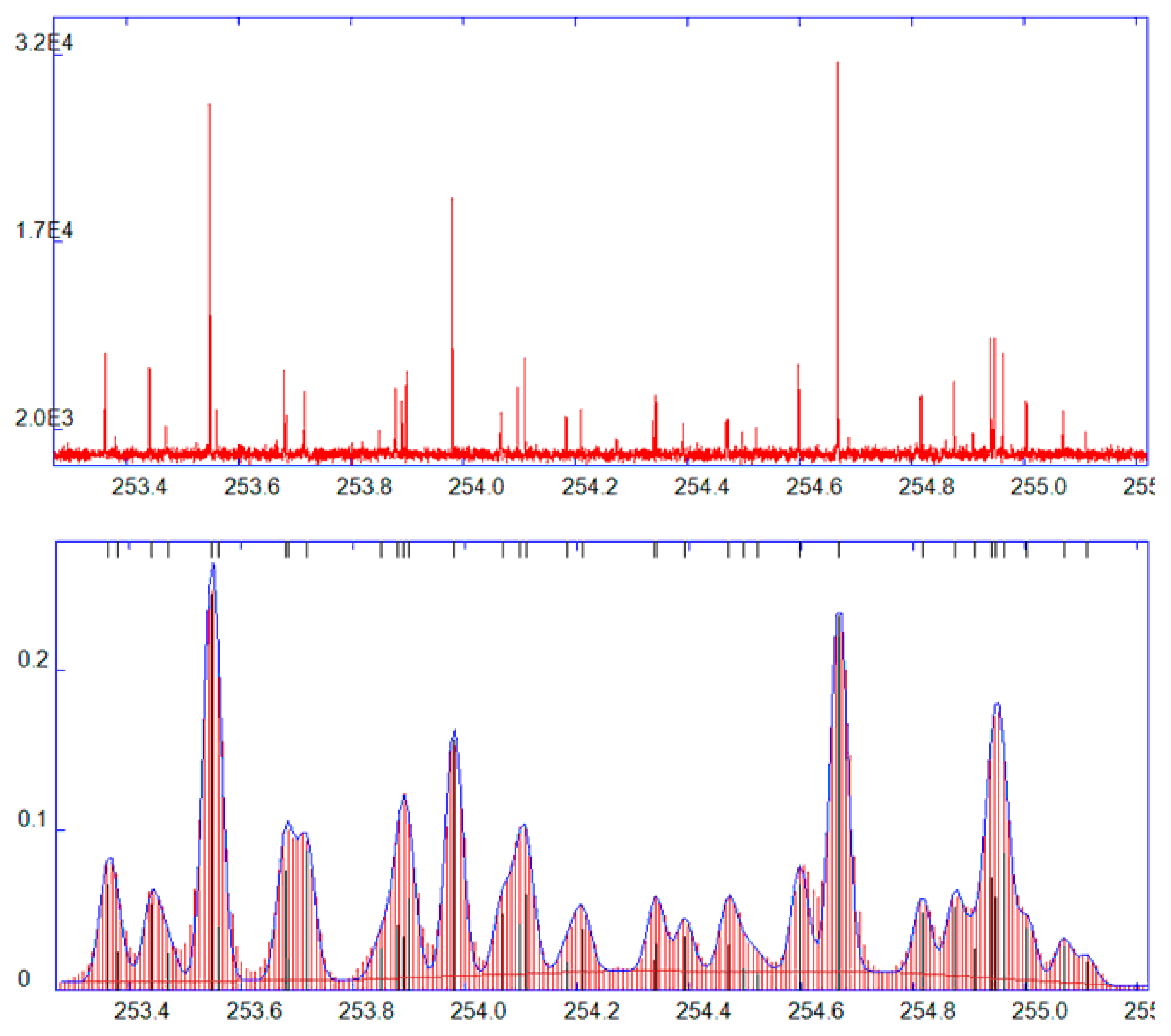
GDOES is essentially an atomic spectroscopy technique, i.e., a typical GDOES spectrum consists of transitions between valence electrons of analyte atoms and singly charged ions. This corresponds to wavelengths in the ultraviolet region, while important emission lines of light elements (H, O, N, C, P, S) have wavelengths below 200 nm (the vacuum UV region), where light is strongly absorbed by atmospheric oxygen. Therefore, vacuum spectrometers or spectrometers flushed with nitrogen are used. At the other end of the spectrum, in the visible region, there are some strong lines of alkali elements that may also be of interest. Spectra of transition elements are line-rich; they may consist of hundreds of lines, see e.g., the spectrum of iron (Figure 3). A good reference, to find and classify spectral lines, is the NIST Atomic Spectra Database [18], freely accessible on the web, or older wavelength tables [19,20]. In analytical applications, it is important to avoid or minimize line interferences (line overlaps), i.e., situations in which a nearby line of another element contributes to the signal of a line intended for analysis of an element of interest. To be able to resolve such interferences, GDOES spectrometers must have a sufficient spectral resolution. Common are large Paschen-Runge polychromators (0.5–0.75 m focal length) [21] with photomultipliers, having the resolution of ≈25–35 pm. Also, smaller spectrometers are used in commercial instruments, typically with CCD detectors, with a resolution around 60–70 pm.

Photomultipliers offer an excellent sensitivity, and their gain can be easily adjusted by the supplied voltage. They are fast, they can register very fast changes of the incident light intensity and have a high dynamic range. A photomultiplier is used for the detection of a single wavelength, either fixed (in a polychromator) or adjustable, in a monochromator, that is sometimes added to a GDOES spectrometer to provide an additional freely selectable analytical channel. On the other hand, CCD arrays offer continuous coverage throughout a certain wavelength range, with the freedom to use any wavelength from that region as an analytical channel. In practical applications, this brings the possibility to use several different analytical lines for an element, which is an advantage. However, the gain of a CCD detector depends on the integration time, i.e., for how long the light is collected in a single measurement. This results in the necessary trade-offs between the sampling rate and sensitivity in depth profiling applications, especially in the analysis of very thin surface layers and low concentrations.

Commercial instruments with photomultipliers are always built to order, with a specific configuration, defined according to the likely analytical applications to be supported. Instruments with CCD detectors are more universal. It is common that all commercial instruments are delivered with at least one analytical application completely set, with the relevant calibrations in place, ready to use. After installation, it is good to check that the performance of that application is in conformity with the beforehand agreed specifications, concerning the accuracy within the specified class of materials, sensitivity and detection limits of the elements under study.

4. GDOES Intensities as Functions of Sample Composition, Analytical Methodology

GDOES is a relative method; it depends on calibration. The calibration must be self-consistent: if a calibration sample is measured as an unknown and the resulting intensities are treated by that calibration, the resulting composition must be in conformance with the certified values. Emission intensities of analyzed elements reflect the processes occurring in the spectral source. In the analysis of a matrix (material) M, the intensity I_λ(E),M of a line λ(E) of element E is proportional to the number density of that element in the plasma, n_E, which is controlled by dynamic equilibrium between the incoming flux of the atoms E from the cathode (=‘source’) and the outgoing flux of atoms that are redeposited on the anode walls (=‘drain’). The incoming flux of an element is proportional to its concentration c_E,M in the analyzed matrix M, and the sputter rate of that matrix, q_M. The redeposition flux is proportional to n_E. (The situation is more complex if the element E exists in the plasma as a gas with a low sticking coefficient on the anode surface [22] (e.g., He [23]), or if the sample under study is structurally inhomogeneous, with strongly different sputter rates of the phases present [24]. Also, immediately after the startup, line intensities are affected by the desorption of atmospheric gases from the anode wall, exposed to air when changing the sample. This might impair the performance in the analysis of thin surface layers). The proportionality relations mentioned above, combined together, result in I_λ(E),M being proportional to the product (c_E,M q_M) [25,26]. The respective proportionality factor is supposed to be independent of the matrix M and is called the emission yield of the line λ(E) and denoted R_λ(E). Besides this, the recorded intensity at this wavelength always contains a spectral background, a contribution not related to the presence of element E. It is usually expressed as a constant b_λ(E). With this notation, we can then write [25]

$$I_{\lambda \left(E\right),M}=R_{\lambda \left(E\right)}\left(c_{E,M}{q}_M\right)+b_{\lambda \left(E\right)}$$

(1)

Some lines exhibit non-linear intensity response as a function of (c_E,M q_M) due to self-absorption [26]. This is typical for the so-called atomic resonance lines, frequently used in GDOES analyses. The most common way to account for this is to add a quadratic term on the left side of Equation (1), i.e.,

$$a_{\lambda \left(E\right)}{I}_{\lambda \left(E\right),M}^2+I_{\lambda \left(E\right),M}=R_{\lambda \left(E\right)}\left(c_{E,M}{q}_M\right)+b_{\lambda \left(E\right)}$$

(2)

where a_λ(E) expresses the magnitude of that non-linearity and is also independent of the matrix M. Equation (1) or Equation (2) thus represents a general relation between the concentration of an analyte element E and the intensity of its line λ(E). These relations are used as follows:

In the process of calibration, a set of reference samples with known composition c_E,M and known sputter rates q_M is measured, intensities I_λ(E),M are collected, and calibration constants R_λ(E), b_λ(E) are established by linear regression, based on Equation (1), or, in case of a non-linear signal response, Equation (2) is used instead of Equation (1), and there is one more calibration constant, a_λ(E). This procedure is performed for all the elements expected to be present in the samples to be analyzed. Then, in the analysis of an unknown sample, intensities of the respective lines of all those elements are measured, and Equation (1) or Equation (2) is used in the reverse way, i.e., the products (c_E,M q_M) are now treated as unknown quantities and are calculated from Equation (1) or (2), using the already known calibration parameters R_λ(E), b_λ(E), a_λ(E). Now, the only step that remains to be done to get the composition of the unknown sample is to establish its sputter rate q_M. However, if all the elements E potentially present in that sample were analyzed, all the products (c_E,M q_M) are known, and we can use the fact that the sum of all the concentrations is close to 100%:

$${\sum }_E c_{E,M} q_M=q_M {\sum }_E c_{E,M}=q_M·\left(100\%\right)=q_M$$

(3)

It is common that relative dimensionless parameters, the ‘sputter factors’, are used instead of the ‘true’ sputter rates (sputtered mass per second), namely, the ‘true’ sputter rate divided by the sputter rate of a reference matrix at the same discharge conditions, usually pure iron: q_M → q_M/q_{pure Fe}. Unlike the ‘true’ sputter rates, sputter factors are either virtually independent of discharge conditions, or their variations with discharge current and discharge voltage are moderate [27,28]. They are material-specific and in the calculations described above, they play the same role as the ‘true’ rate: if all the sputter rates in a calibration, Equation (1) or Equation (2) are multiplied by the same constant, let it be denoted k, i.e., q_M → k.q_M, all that happens is that the regression parameters R_λ(E) change themselves into R_λ(E)/k, and the correspondence between emission intensities and the composition of the samples remains unaffected. It is common to express all the concentrations in weight percent (% m/m), and this convention is followed throughout this paper, unless indicated otherwise.

5. Example of an Application-Specific Calibration: Analysis of Boron

The methodology described in the previous section will be demonstrated by the analysis of boron in two depth profiling applications: (1) B-doped diamond layers prepared by chemical vapor deposition, and (2) magnetron sputtered W-Ni-B coatings. The calibration should cover reasonably well the expected concentration ranges of all the elements of interest, and calibration samples must be chosen accordingly. Sputter factors are usually known for some of those standards only; such a set is sometimes called the calibration base. An efficient way of establishing sputter factors for the remaining standards is to calculate them based on the already existing calibration curves, established by the samples of the calibration base. By this method, it is possible to extend the (usually limited) concentration ranges covered by the calibration base to become suitable for the requested analytical application [25,29]. The calculation of the sputter factor q_M of a specific calibration sample M involves linear regression [30]: the weighted error function ${\chi }_M^2$ to be minimized, for calibration functions described by Equation (1), is

$${\chi }_M^2={\sum }_F{w}_{\lambda \left(F\right),M}{\left(I_{\lambda \left(F\right),M}-R_{\lambda \left(F\right)}{c}_{\lambda \left(F\right),M}{q}_M-b_{\lambda \left(F\right)}\right)}^2$$

(4)

where w_λ(F),M are statistical weights, and the summation (index F) proceeds over the channels belonging to the calibration base. This is the same type of calculation as when calibration parameters R_λ(E), b_λ(E), are being established, based on Equation (1), except that, instead of considering calibration points of different samples belonging to the same channel, points belonging to the same sample, M, are considered here, coming from different channels of the calibration base. The weighting in Equation (4) must reflect different sensitivities (emission yields) in different channels and different concentrations of the elements constituting the calibration base. This can be satisfied, e.g., by the following weights: w_λ(F),M = 1/(R_λ(Fc_F,M))².

In this experiment, six standards of low alloy steels + pure iron, with known sputter factors, were available, see

Table 1. Calibration samples (reference materials) used in the analysis of B-doped diamond. Samples included in the calibration base (low alloy steels) are highlighted by a light blue background. Bold script (black): high enough contents of C, B for the calibration. Bold script (blue): by these concentrations the last four standards differ from low alloy steels. Element concentrations are in weight pecent (% m/m).

Ref. Material	Supplier	qM	Fe	Cr	Ni	Mn	Co	W	Al	Ti	Mo	Si	C	B
180A	ČKD	1.00	99.98	0.004	0.001	0.001	0.0002	0.001	0.0001	0.001	0.004	0.0004	0.003	0.0001
183A	ČKD	1.056	94.5	0.204	1.09	1.74	0.119	0.354	0.15	0.003	0.036	1.02	0.047	0.0005
188A	ČKD	1.137	90.6	5.11	0.445	0.169	0.006	0.091	0.093	0.034	1.28	0.775	0.332	0.0047
1761	NIST	0.95	95.0	0.22	1.99	0.678	0.028		0.055	0.18	0.103	0.18	1.03	0.002
1762	NIST	1.00	94.1	0.92	1.15	2.00	0.062		0.069	0.095	0.35	0.35	0.337	0.0049
1763	NIST	1.00	95.0	0.50	0.51	1.58	0.095		0.043	0.31	0.50	0.63	0.203	0.0054
15254-Z	MBH	1.037	91.7	2.12	0.394	1.12	0.55	0.349	0.599	0.303	0.758	0.916	0.285
1837A	MBH	1.402	0.10	9.98	65.8	0.003	10.0	0.012	5.63	5.28	3.00	0.053	0.004	0.11
SP3C_bor	SPL	0.978	73.8	16.4	5.31	0.43	0.041	0.12	0.095	0.17	0.26	0.84	0.30	1.67
Atabor	Vítkovice	0.973	65.8	19.4	11.7	1.29	0.040					0.42	0.014	1.19
244B	ČKD	0.827	93	0.36	0.336	0.68	0.049	0.052	0.019	0.019	0.056	2.06	2.57	0.093

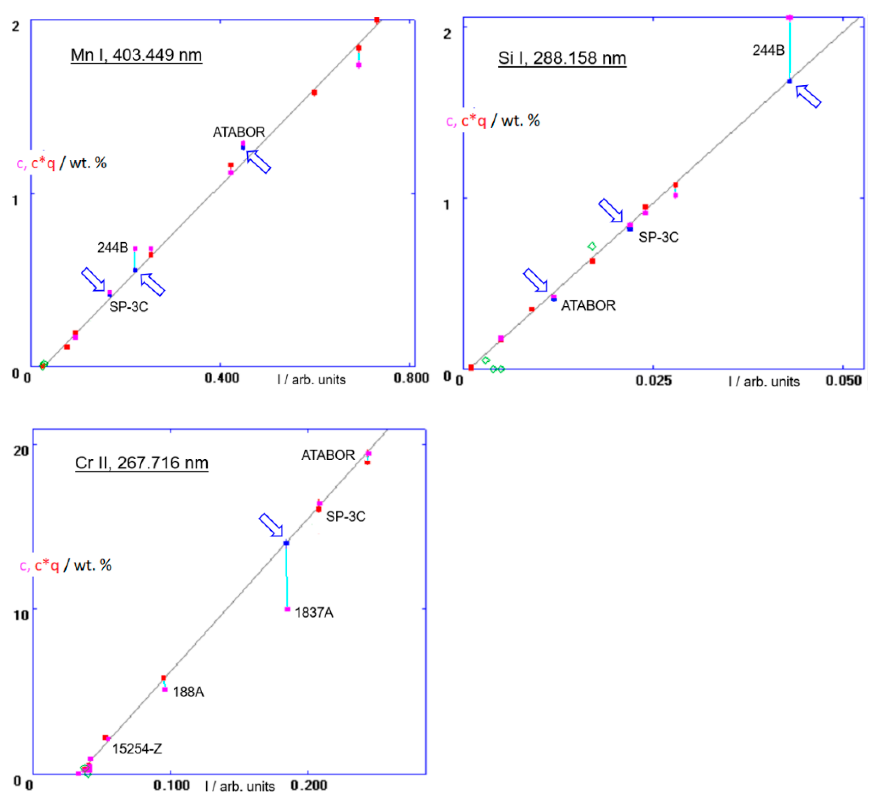
ČKD: ČKD Technical Laboratories, Praha, Czech Republic; NIST: National Institute of Standards and Technology, Gaithersburg, MD, USA; MBH: MBH Analytical Ltd., Barnet, EN5 4DJ, UK; SPL: SPL-Labmat s.r.o., Bohumín, Czech Republic; Vítkovice: Vítkovice a.s., Ostrava-Vítkovice, Czech Republic.

. To allow for the analysis of B-doped diamond, four more standards with higher boron concentrations were selected: 1837A, SP-3C, ATABOR and 244B. The last one also has a high carbon content, which allows the calibration of carbon to become suitable for diamond. All the measurements were done with a dc discharge at 800 V, 15 mA, with a 2.5-diameter anode. First, the sputter factors of samples SP-3C, ATABOR and 244B were established using the Mn 403, Si 288 channels and a calibration base consisting of the steel standards mentioned above. (The designation of a channel consists of the element symbol and an abbreviated wavelength in nm. Actual wavelengths of the lines used are in the calibration plots). The sample 1837A has very low concentrations of both manganese and silicon, so, in the second step, the samples SP-3C and 244B, with the already established sputter factors, were added to the calibration base and the sputter factor of the sample 1837A was calculated, based on the thereby established calibration function of the channel Cr 267. The mentioned calibration functions are plotted in Figure 4. In these plots, emission intensities are plotted on the X-axis, and the quantities on the Y axis are (1) concentrations c_E,M (magenta points) and also (2) sputter rate-corrected concentrations, (c_E,Mq_M), of the calibration samples. Those belonging to the calibration base are represented by red points, and those already calculated are marked by blue points, i.e., in this notation, each calibration sample is represented by a red (or blue) point and a magenta point, connected by a vertical line. 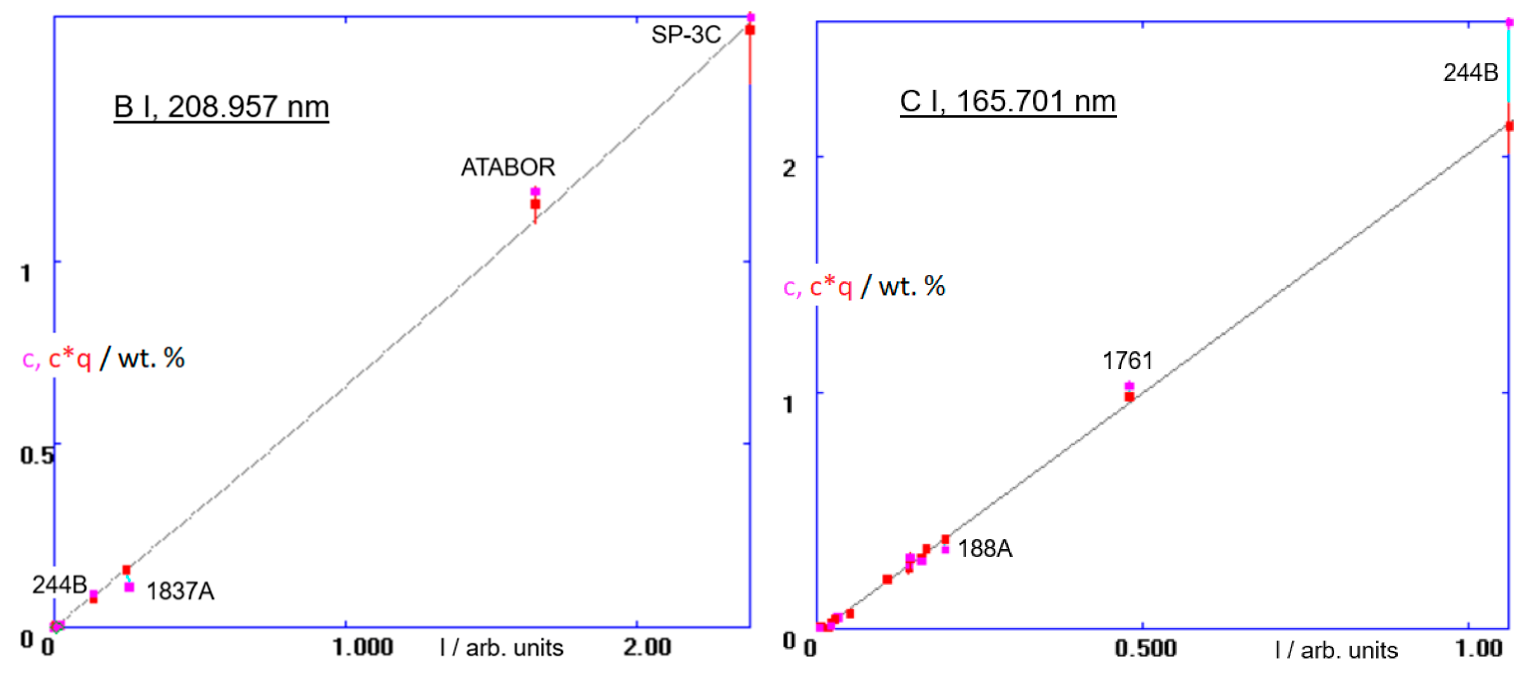For samples with q_M close to 1.00, the two points of the pair (almost) coincide. The valid calibration curve is then defined by red points belonging to different samples. The resulting sputter rate-corrected calibrations of boron, the B 208 channel, and that of carbon, C 165, are in Figure 5.

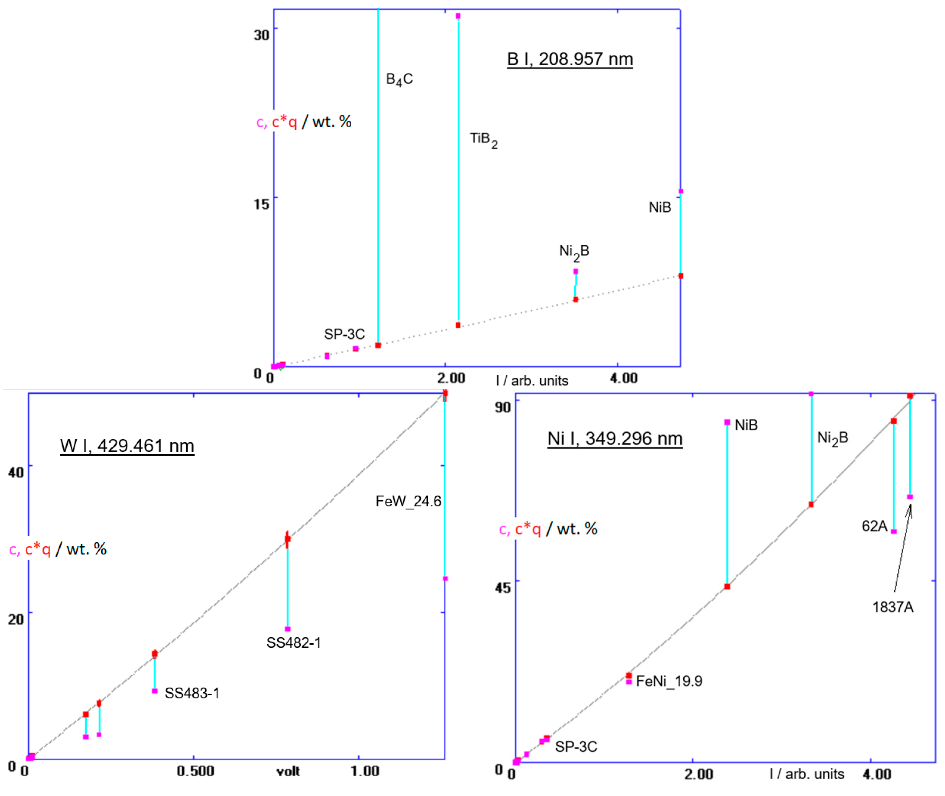
A more complex matrix than the B-doped diamond is magnetron sputtered W-Ni-B metallic glasses [31]. Not only is this a ternary system, but there are also much higher boron concentrations than in B-doped diamond. The stoichiometry of these layers needs to be thoroughly controlled. For that purpose, the previously described calibration was further extended, and sputter factors of additional standards were calculated in a series of steps similar to those two described above. They are listed in

Table 2. Additional calibration samples (reference materials) to extend the calibration from Table 1 for analysis of W-Ni-B metallic glasses. Cell background colours: grey: high-speed steels, yellow: Fe-Me binaries, white: nickel matrix, magenta: borides. Bold script: concentrations by which the extended calibration ranges are covered. Element concentrations are in weight pecent (% m/m).

Ref. Material	Supplier	qM	Fe	Cr	Ni	Mn	Co	W	Al	Ti	Mo	Si	C	B
SS482-1	BAS	1.771	75.4	3.95		0.26	0.29	17.83			0.40	0.14	0.675
SS483-1	BAS	1.542	84.3	2.90		0.22	2.06	9.28			0.18	0.16	0.65
FeNi_19.9	MBH	1.073	80.1		19.9
62A	ARMI	1.478	1.08	19.4	57.2	0.02	13.3	0.11	1.32	3.05	4.33	0.05	0.039	0.005
RNi10-6	SUS	1.50	<5 ppm		99.99								<0.001
FeTi_15	MBH	0.855	85							15
FeW_24.6	MBH	2.088	75.4					24.6
B4C	RHP	0.024											21.7	78.3
TiB2	RHP	0.117								68.9				31.1
Ni2B	RHP	0.698			91.6									8.43
NiB	RHP	0.517			84.5									15.6

BAS: Bureau of Analysed Samples Ltd., Newby, Middlesbrough, TS8 9EA, UK; ARMI: Analytical Reference Materials International Inc., Evergreen, CO, USA; SUS—Ulrich Nell GmbH., Oberhausen, Germany; MBH: MBH Analytical Ltd., Barnet, EN5 4DJ, UK; RHP Technology GmbH., Austrian Res. Ctr., Seibersdorf, Austria.

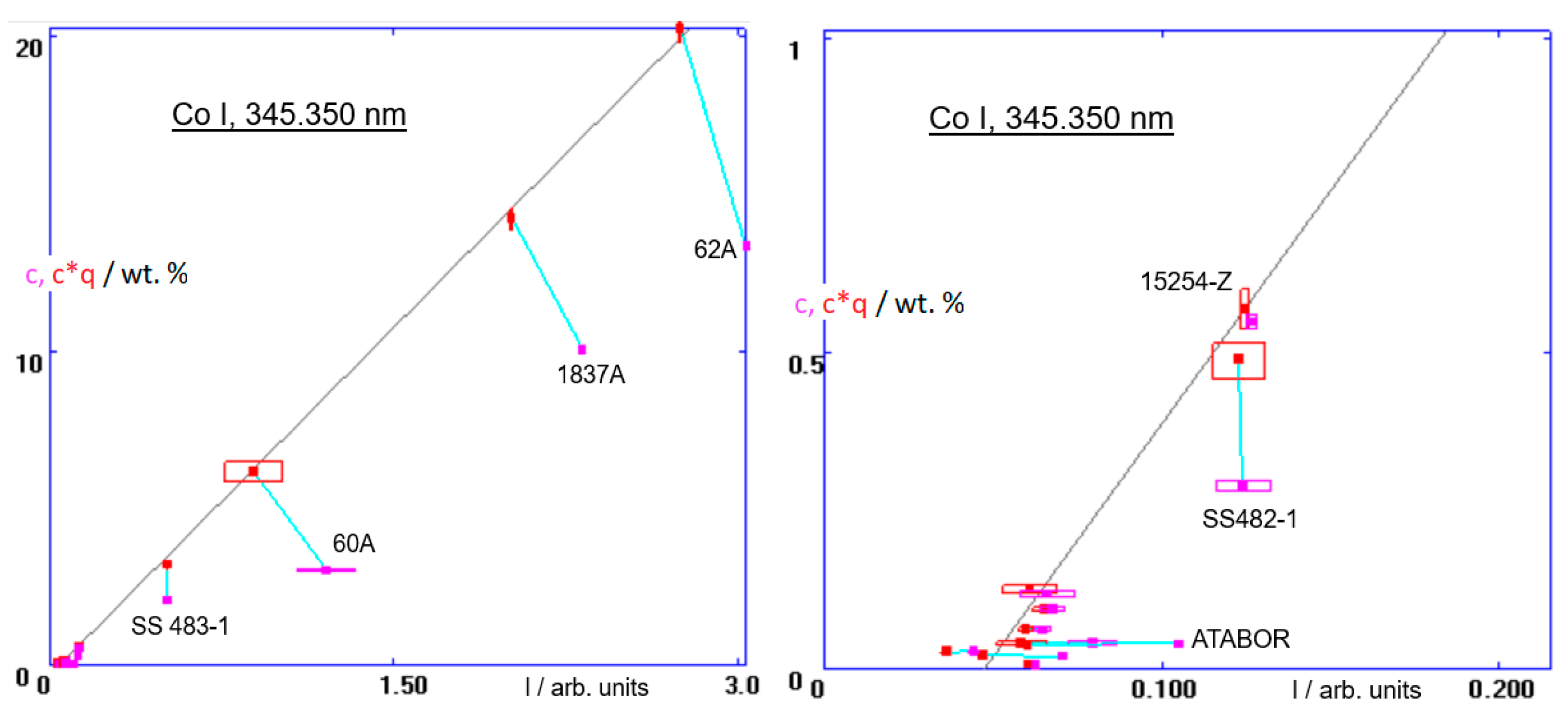
. In Figure 6 are the resulting calibration functions of the B 208, W 429 and Ni 349 channels (The abscissa scaling in the plot of the B I, 208.957 nm line is here different from that in Figure 5). For completeness, it is worth showing also the calibration of the Co 345 channel, which is a part of this method (A system of interrelated calibrations, using the same calibration samples and intended for a specific application, is frequently called a ‘method’. Usually, also elements that do not necessarily occur in the anticipated unknown samples need to be included, to provide a reference for prospective corrections of line interferences with the lines of the elements of interest, see Figure 7). The Co I, 345.350 nm line has an interference with a nearby line of nickel. The contribution to the measured intensity from nickel must be subtracted, in a way described in Ref. [25]. Thereby, the red points in the calibration diagram are shifted horizontally to the left. This results in sloping connections between the uncorrected (magenta) and the corrected (red) points, instead of vertical. It is vital to use correct line interference corrections, especially as it is in the analysis of minor elements [32].

Finally, a remark should be made about sputter factors/sputter rates. B-doped diamond has an extremely low sputter rate, ≈40 times lower than iron. This is why both carbon and boron can be analyzed in those coatings using calibrations involving much lower concentrations of these elements in ferrous standards, generating, however, comparable intensities. Also, the sputter factor of boron carbide, B₄C, is low (q_M = 0.024), see the calibration in Figure 6. Sometimes it may be beneficial to work with a different discharge gas than argon [33]. Figure 8 is a comparison of sputter factors of different matrices in an argon and a neon discharge. Here is this presented mainly to show over how a wide range the sputter factors of different matrices span. There is a big difference between sputter rates in GDOES and sputter rates in the ion-beam or magnetron sputtering: in GDOES, the (net) rate is strongly affected by redeposition, unlike high-vacuum methods, and even relative sputter factors of different matrices in both setups may strongly differ.

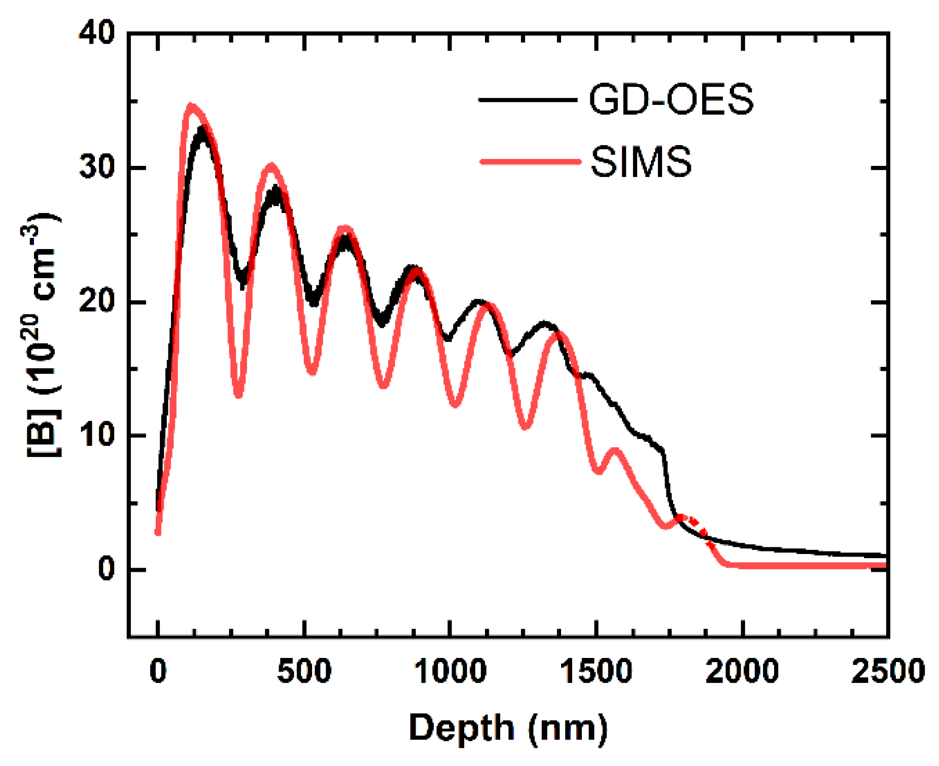
An example of an actual quantitative depth profile of B-doped diamond multilayer analysed by GDOES, together with a parallel result measured by secondary-ion mass spectrometry (SIMS), is in Figure 9. Maximum boron concentration in the multilayer, ≈33 × 10²⁰ atoms/cm³, corresponds to 1.97 wt.% B, with an estimated density of PVD-deposited diamond of 3.4 g cm⁻³. Depth quantification of the profiles will be discussed in Section 7.

6. Uncertainty Considerations

The issues of accuracy and precision can be treated by general rules of error propagation [35]. For linear intensity response without line interferences, Equation (1), and if a single line is used for element E and the uncertainty of q_M is not considered, the partial relative uncertainty f_E,M = δc_EM/c_EM associated with the analysis of element E at a concentration high enough that b_E can be neglected, will be

$$f_{E,M}^2={\left({\displaystyle \frac{\delta I_{E,M}}{I_{E,M}}}\right)}^2+{\left({\displaystyle \frac{\delta R_E}{R_E}}\right)}^2$$

(5)

where the first term on the right side expresses random uncertainty of the intensity measurement, and the second term is the systematic error due to a prospectively biased emission yield, coming from calibration. In this paragraph, concentrations are expressed as mass fraction instead of percent. Because of normalization to 100%, Equation (3), an error in the analysis of any element will affect all the other elements as well. Contributions to the relative error of c_E,M caused by errors in intensities and emission yields of the other elements are proportional to their concentrations [25]:

$${\left({\displaystyle \frac{\delta c_{E,M}}{c_{E,M}}}\right)}^2={\left(1-c_{E,M}\right)}^2{f}_{E,M}^2+{\sum }_{F\ne E}{c}_{F,M}^2{f}_{F,M}^2$$

(6)

For minor elements, at concentrations close to the detection limit, the spectral background, b_E, becomes important and the uncertainty δc_E,M of a minor element can then be expressed as [25]

$${\left(\delta c_{E,M}\right)}^2={\displaystyle \frac{{\left({BEC}_E\right)}^2}{q_M^2}}\left[{\left({\displaystyle \frac{{\delta I}_{E,M}}{b_E}}\right)}^2+{\left({\displaystyle \frac{\delta b_E}{b_E}}\right)}^2\right]$$

(7)

where

$${BEC}_E={\displaystyle \frac{b_E}{R_E}}$$

(8)

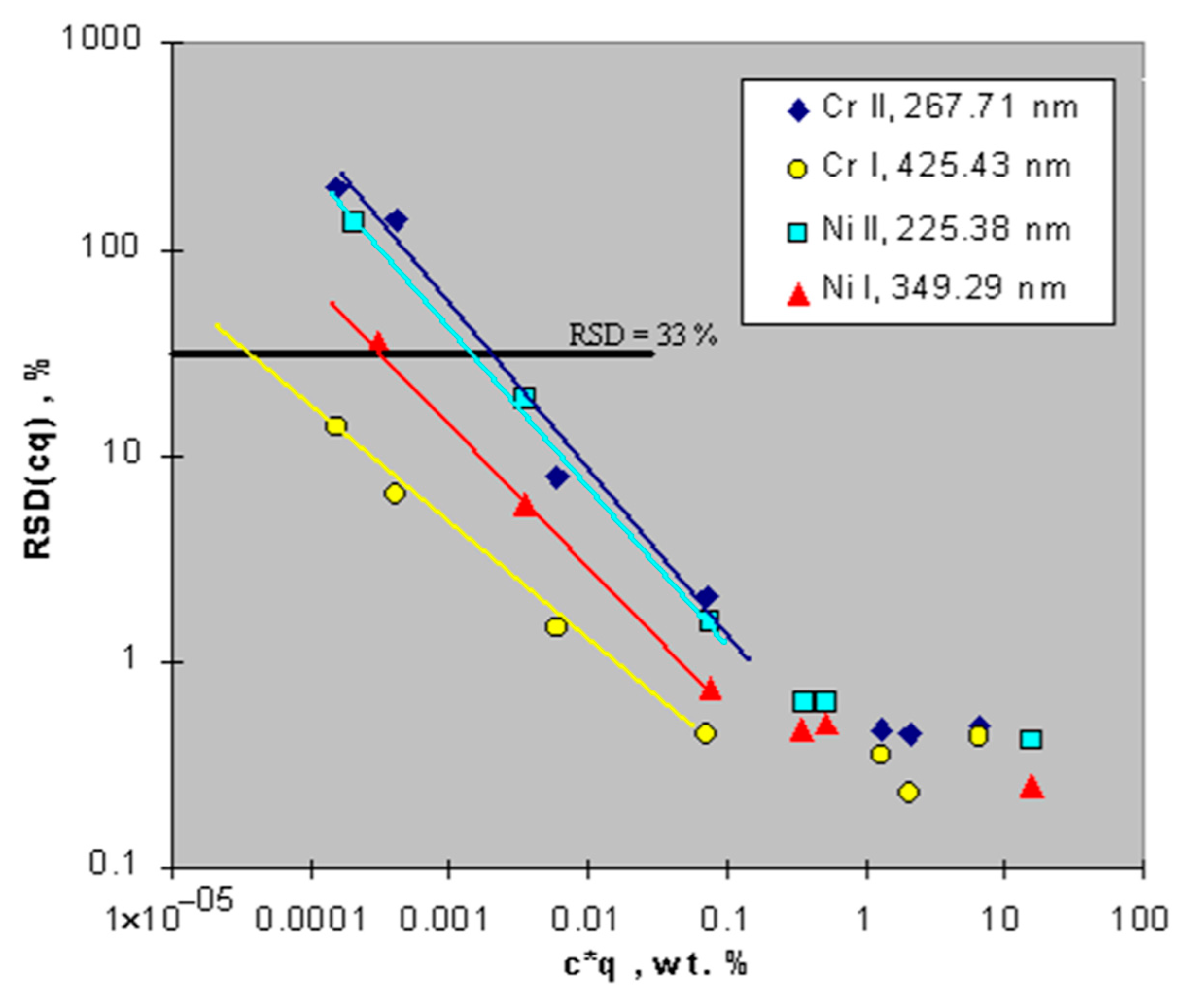
is the background equivalent concentration of element E. In the square bracket on the right side of Equation (7), the first term expresses the random uncertainty of the intensity measurements of element E relative to the background b_E, and the second term is the systematic relative error, due to a prospectively biased background b_E, as resulting from calibration. The detection limit of an element depends on the relative strength of the line used for its analysis, see the plot in Figure 10. Typical detection limits in GDOES, element-specific, are between 1.0 and 100 ppm (m/m).

In the analysis of coatings by GDOES, random uncertainties are usually not critical (it is unique that, by GDOES, it is quick and easy to do replicate measurements, unlike virtually any other depth profiling method). The variability of the resulting depth profiles is typically due to real variations of the coating throughout the analyzed area, provided that the area is big enough to enable such measurements. Much more of concern is accuracy, i.e., the chance that the results will be systematically biased. So far, all the considerations concerned errors within the standard calibration model, Equations (1) and (2). It is critical to implement it properly, i.e., to make sure that the correct sputter factors of the calibration samples are used, as well as relevant corrections for line interferences and non-linear intensity functions, wherever necessary. Also, the problem with coatings is that often rather unusual compositions are to be analysed, for which no matrix-matched standards exist. How to cope with that was shown in the example of W-Ni-B metallic glass coatings in Section 5. The GDOES standard calibration model, Equations (1) and (2), is rather robust; it works well for a wide range of matrices. It is, however, important to make sure that the composition of the calibration standards used spans the full range of the anticipated compositions of unknown samples to be analysed. Especially dangerous are attempts to extrapolate non-linear calibrations far beyond the actual calibration range. This usually leads to unacceptable errors. Also, it is worth to mention that, if using a resonance line with non-linear intensity response expressed by quadratic approximation, Equation (2), with a_λ(E) > 0, the slope of the calibration curve I_E,M = I(c_E,M) goes up as the concentration c_E,M rises, and, in the analysis of unknown samples, even the random component of the uncertainty δc_E,M becomes higher than in case of a linear calibration function with the same R_E. This becomes apparent if Equation (5) is modified to reflect a quadratic calibration function I_E,M = I(c_E,M), as expressed by Equation (2), without even considering the uncertainty δa_λ(E):

$$f_{E,M}^2\cong {\left({\displaystyle \frac{\delta I_{E,M}}{I_{E,M}}}\right)}^2\left[1+4a_E^2{I}_{E,M}^2\right]+{\left({\displaystyle \frac{\delta R_E}{R_E}}\right)}^2$$

(9)

The GDOES standard calibration model is relatively robust, but not universal. There are deviations from it, usually called the ‘matrix effects’. The most reliable lines, with minimal matrix effects, are atomic resonance lines with low excitation energies. On the other hand, when working with ionic lines (Me II), caution is needed, see e.g., [25,26,36]. The most recommended way to avoid matrix effects and errors due to problems with calibration within the standard model (e.g., missing line interference corrections, biased calibration parameters, etc.) is to use several different lines for an element. If all those lines give the same (c_E.q) values in the analysis of unknown samples, it is very likely that the analysis is correct. A specific category is matrix effects caused by light elements such as H, N, O [37,38], the discussion of which is beyond the scope of this review. 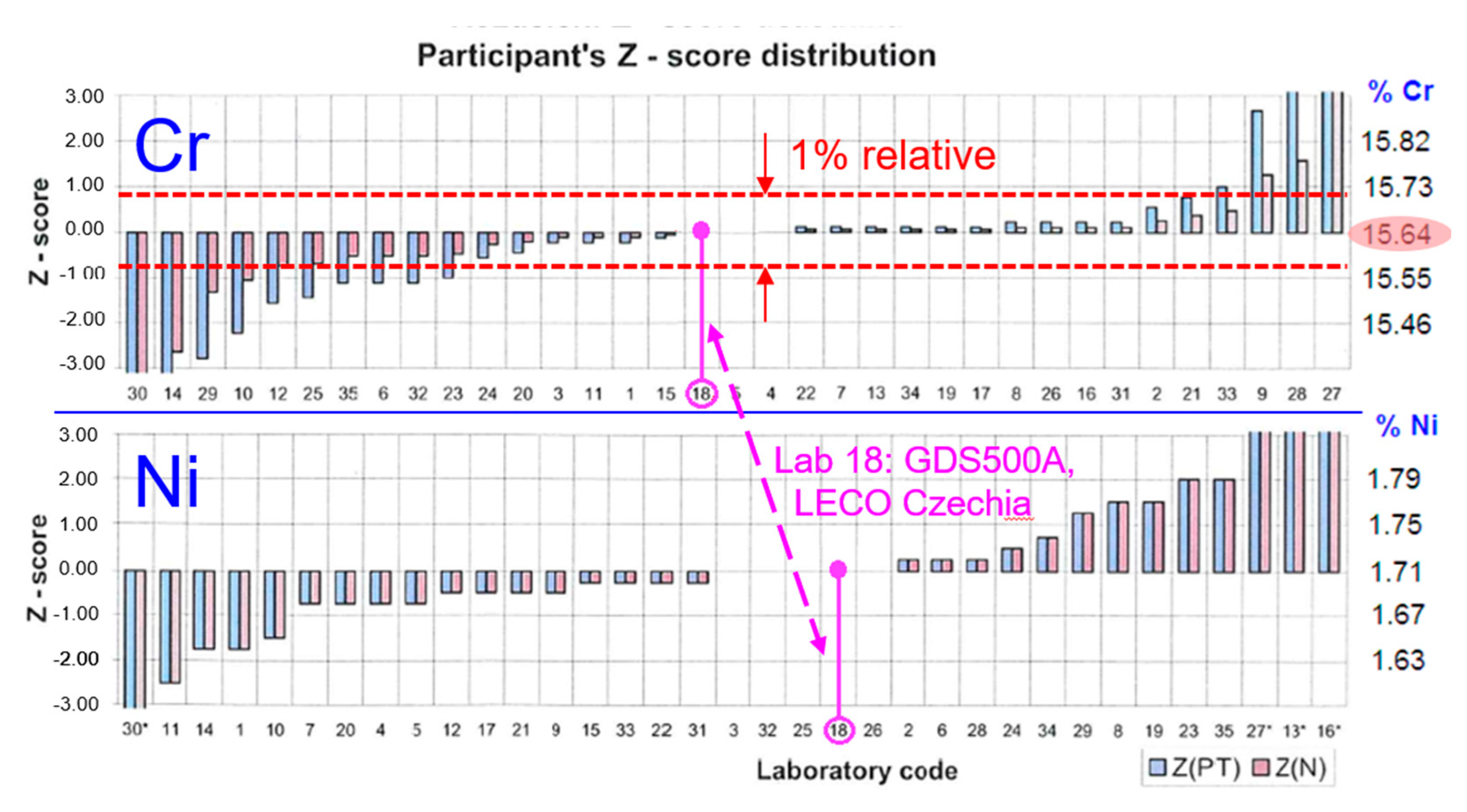In analytical science, there is a well-established general system of checks and procedures to achieve good accuracy and characterize reference materials, based on anonymized inter-laboratory comparisons (‘round robin’ experiments, proficiency testing) [39]. An example of the distribution of results reported by laboratories participating in such a test, in the analysis of the 16Cr2Ni stainless steel [40], is in Figure 11. The mutual compliance of the results is remarkable: in the analysis of chromium, 21 out of 35 laboratories from 3 countries, using different methods, reported results within the margin of 1% relative around the reference value (the median of the whole set). As a measure of the ‘proficiency’ of an individual lab, the Z-score is used, defined as

$$Z={\displaystyle \frac{x-\mu }{\sigma }}$$

(10)

where x is the reported result, μ is the reference value, and σ is the standard deviation of the whole set, with outliers removed. The smaller the absolute value of Z, the better the reported result.

7. Depth Quantification, Crater Effect

In depth-profiling applications, emission intensities in the analysis of an unknown sample are recorded as functions of the time of sputtering, t. From calibration relations, Equation (1) or (2), when they are applied to the intensities, I_λ(E),M(t), it is possible to obtain the composition also as a function of time, c_E,M(t). From Equation (3), it is then possible to obtain also the sputter rate as a function of time, q_M(t). The mass of the sample sputtered in the time interval dt will then be

$$dm={\rho }_M·\pi r^2·dh=q_M\left(t\right)dt$$

(11)

where ρ_M is the density of the cathode (sample) material and r is the anode radius (i.e., the radius of the erosion crater). The depth h(t) as a function of the time of sputtering can then be established by integrating Equation (11):

$$h\left(t\right)={\displaystyle \frac{1}{\pi r^2}}{\int }_0^t{\displaystyle \frac{q_M\left(\tau \right)}{{\rho }_M}}d\tau$$

(12)

The resulting depth profile can then be plotted as a function of h instead of t, so that prospective variations of the sputter rate across the profile are accounted for. In such calculations, the density of the layer under study is either known or various approximate estimates can be applied, relating the density to the composition at the specific depth. Subsequently, this can be verified by measuring the crater depth when the analysis is over. Another possibility is to measure the depth profile of a thickness standard of a known matrix with known thickness, and adjust the depth quantification accordingly, see the depth profile of a Kocour thickness standard of Fe coating on steel, Figure 12.

The integration of Equation (11) can be simplified in an important task of establishing the surface coverage by an element E, μ_E, in terms of mass-per-area, instead of layer thickness. If the element of interest is concentrated close to the surface and vanishes deeper in the sample, the upper limit of the integral can be chosen deep enough, and, if the background b_E is negligible, Equations (11) and (1) give

$${\mu }_E={\displaystyle \frac{1}{\pi r^2}}\int c_{E,M}\left(t\right)dm={\displaystyle \frac{1}{\pi r^2}}{\int }_0^{\infty }{c}_{E,M}\left(t\right)q_M\left(t\right)dt={\displaystyle \frac{1}{\pi r^2}}{\int }_0^{\infty }{\displaystyle \frac{I_{E,M}\left(t\right)}{R_E}}dt$$

(13)

i.e., it is sufficient to integrate the bare intensity I_E(t), divided by the emission yield and the crater area (both are constants). The advantage is that, in this approach, it is not necessary to know the density ρ_M, as density controls only the depth scale, which is, in this case, irrelevant. If the sample has a big enough area, it is relatively easy to do replicate measurements of this kind, and look at the resulting statistical distribution {μ_E} in a similar way as treating the results of bulk analysis, Figure 10. In a recent application in which surface contamination of steel by boron was examined, the limit of detection for boron on the surface was found to be ≤0.1 mg m⁻². Integration similar to Equation (13) can also be used to quantitatively assess the contamination or segregation of an impurity at a substrate-coating interface, provided that its concentration on both sides, farther from the interface, is negligible.

The interpretation of Equation (12), as presented above, holds accurately only if the erosion crater has perfectly straight walls, perpendicular to the sample surface, and a perfectly flat bottom. In GDOES, this never happens; glow discharge sputtering is laterally uneven, while the shape of the crater depends on discharge conditions [27] and can be optimized, to some extent. Because of this, material originating from different depths enters the plasma simultaneously, distorting thereby the resulting depth profile (the crater effect). In a virtually homogeneous material, sputter rate does not change with depth, but differs in different positions within the erosion crater. As the crater deepens, its shape, if expressed in relative depth units, virtually does not change with time. At such situation, intensity response I_E(t) will depend on the actual depth distribution c_E(h) of element E as follows [41,42]:

$$I_E\left(t\right)=K{\int }_0^1{F\left(u\right)c}_E\left(ut\right)du$$

(14)

where K is a constant and the variable u denotes relative depth, so that u = 1 at the deepest part of the crater and u = 0 at the (original) surface. F(u) is the weight function, expressing relative contribution to the measured signal from the material originating at the depth u. The narrower the peak of F(u), the smaller is the distortion of the depth profile by the crater effect. The constant K can be established by normalization, so that in the analysis of a sample with element E distributed homogeneously with depth, the integral in Equation (14) should be equal to c_E. The weight function can be established from the intensity response I_δ(t) of a very thin layer (a marker) of element E, buried at a certain depth, which is reached by the deepest part of the crater at the time t₀:

$$F\left({\displaystyle \frac{t_0}{t}}\right)={\displaystyle \frac{1}{K}}{tI}_{\delta }\left(t\right),\hspace{1em}for\hspace{1em}t\ge t_0$$

(15)

Alternatively, a sharp interface between a layer of a different material on a substrate containing a homogeneously distributed element E can be used; in that case, the relation between the intensity response of element E, I_Y(t), and the weight function F, will be

$$F\left({\displaystyle \frac{t_0}{t}}\right)={\displaystyle \frac{1}{K}}{\displaystyle \frac{t^2}{t_0}}{\displaystyle \frac{d}{dt}}{I}_Y\left(t\right),\hspace{1em}for\hspace{1em}t\ge t_0$$

(16)

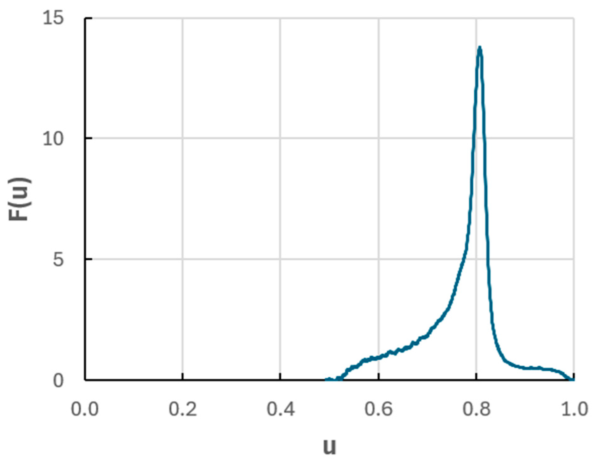
The restoration of true profiles based on the intensity response described by Equation (14), by a numerical procedure, is difficult, and the solution for a general distribution c_E(h) is not available. It is, however, feasible, to estimate additional broadening by the crater effect of depth profiles describing, e.g., coating-substrate interdiffusion [32,41,42]. An example of an experimental weight function F(u) is in Figure 13. It was established using Equation (15) from the intensity-time profile of silicon in the thickness standard of Fe-on-steel, mentioned above (Figure 12). The substrate surface was contaminated or intentionally enriched by silicon prior to deposition, and the Si signal response can be treated as a marker layer. Manganese occurs at a low concentration in the substrate only, not in the Fe layer. It can be shown by using Equation (14) and the weight function from Figure 13, that the profile of manganese, as distorted by the crater effect, will be the same as that in the plot in Figure 12, provided that Mn concentration jumps at the interface from zero to a constant level in the steel substrate. Aluminum is also a minor element in steel, and, in addition to that, an enrichment by Al of the interface is also apparent. Pure iron has a similar matrix as unalloyed steel, with a similar sputter rate and density, so the use of Equation (15) is justified. Otherwise, a correction for the changing material parameters at the interface would have to be made, see Equation (12). In the present example, the deepest point of the crater reached the interface at t₀ = 268 s and the flattest region (the peak of the Si signal) at ≈333 s. This corresponds to the maximum of F(u) at u = 0.81. The mean sputter rate, represented by the integral ∫u.F(u)du, corresponds to u = 0.77, i.e., it is by ≈5% lower. Intuitively, this can be assessed by the plot of F(u), Figure 13: the wing left of the peak of F(u) is bigger than the wing to the right, towards higher u.

As follows from the explanation above, the magnitude of the distortion (broadening) of GDOES depth profiles by crater effect is proportional to the sputtered depth, and, a typical depth resolution, defined as the apparent width of a sharp interface [41], is between ≈8% and 15% of the total depth (=the depth at which the depth resolution is established). The bigger the difference between the sputter rates of the layer and the substrate, the worse is the profile broadening at the interface. An attempt was made to relate the weight function F(u) to the shape of the erosion crater [41,42], however, without considering how relative contributions to the emission intensity depend on the radial coordinate (the distance from the source axis) of the place where the material is sputterred [43]. This, and also the shape of the erosion crater itself, depend on the interplay between the transport of the sputtered atoms within the plasma and their redeposition. Besides the crater effect, other profile broadening mechanisms may be relevant, such as texture development due to a different crystal orientation in a polycrystalline material [44,45] or its structural inhomogeneity [24]. However, in most cases, the crater effect is by far the most prevailing profile broadening mechanism in GDOES. It is also worth to mention that intensity response affected by crater effect cannot be expressed as convolution of the true depth profile c_E(z) with a ‘resolution function’ g(z-z’), like profile broadening in other depth profiling methods. An attempt to do so would require a resolution function depending also on the depth itself, i.e., g(z, z-z’), and the resulting formula would not be convolution, but a different transform, with a completely different mathematics behind.

8. GDOES and Related Methods

For the validation and possible extension of analytical information concerning a system under study, it is always recommended to consider, besides GDOES, also other relevant methods. Some of them are mentioned here. Closely related to GDOES is the Glow Discharge Mass Spectrometry (GD-MS) [46]. It also uses a glow discharge atomization/ionization source, and recorded is the mass spectrum of the ions extracted from the glow discharge plasma. High-resolution magnetic sector instruments or time-of-flight (TOF) spectrometers are used. The former are well suited for the analysis of trace impurities in metals and semiconductors, with a sensitivity by several orders of magnitude better than that of GDOES, and the latter are suitable for multi-element depth profiling of coatings, see e.g., Ref. [47], as TOF-MS instruments allow a fast acquisition of complete mass spectra.

Most materials science laboratories are equipped with a scanning electron microscope with an analyzer of X-ray radiation, generated in the sample by impinging electrons. The X-ray spectrum reflects element-specific radiative transitions and can be used to identify the elements present. The method is known as the Electron Beam Analysis [48], it is quite common, and, depending on the type of analyzer, it is called the Energy-Dispersive or Wavelength Dispersive X-Ray Spectroscopy (EDS, WDS). Unlike GDOES, these methods allow microanalysis, with a μm-range lateral resolution. This allows the line-scan analysis of a cross-section of a coating on a substrate, i.e., it is applicable to the analysis of thicker coatings. However, common analytical figures of merit, such as accuracy and sensitivity, are inferior to those of GDOES, and the analysis of light elements is limited. The method also allows semiquantitative standardless analysis by the so-called ZAF corrections [49]. A limiting factor in the analysis of thin coatings is the information depth, typically in a μm range. A complementary method to EDS/WDS, suitable for the analysis of light elements, is the Electron Energy Loss Spectroscopy (EELS) [50], performed in transmission electron microscopes. However, the preparation of the samples (thin foils) for EELS is not easy when it comes to coating-substrate systems.

Important methods for the analysis of coatings and surface-modified materials are electron spectroscopies (Auger Electron Spectroscopy, AES, [51,52], and X-ray Photoelectron Spectroscopy, XPS, [51]). They are combined with ion beam sputtering as a means to do depth profiling. AES uses as a probe an incident electron beam, XPS a photon beam, and the detected electrons are secondary electrons with energies characteristic of the elements present in the sample, i.e., electrons that do not suffer an inelastic collision before leaving the sample surface. The mean free path of such electrons in a solid is very short (<≈10 monolayers), and so low is also the information depth of these methods. This is their main advantage. Quantification is rather poor compared to GDOES, and ultra-high vacuum is needed to minimize the adsorption of residual gases on the analyzed surface. Besides elemental composition, XPS spectra also carry information about the oxidation state (valence state) of the elements present, which may be of interest. Another surface-sensitive method is the Secondary Ion Mass Spectrometry (SIMS) [51]. It uses the ions ejected from the sample surface due to ion-beam bombardment. Here, the primary ion beam acts as a probe, and, at the same time, it also acts as the means to uncover deeper layers, as the surface is continuously sputtered off. Ion beam sputtering in the depth profile analysis by SIMS, AES and XPS is typically around two orders of magnitude slower than glow discharge sputtering in GDOES. By GDOES, it is possible to routinely analyze depth profiles down to many tens of microns, whilst the methods based on ion-beam sputtering are limited to a few micrometers at most.

It is also worth mentioning accelerator-based methods using high-energy ion beams, with energies in the MeV range. Their accessibility is limited to a few facilities; however, they can provide an independent quantitative information, based on a fundamentally different physics than that of GDOES. In Rutherford Backscattering Spectroscopy (RBS) [53], the sample is irradiated by H+ or He+ ions, and the energy spectrum of elastically backscattered ions contains information about the elements present and their depth distributions. The method is limited to simple matrices, containing only a few elements, and the best performance it delivers in the analysis of a heavy isotope in a matrix consisting of lighter atoms.

In Nuclear Reaction Analysis (NRA), the sample is bombarded by energy-monochromatized ions that may induce a nuclear reaction with a nuclide in the sample to be analyzed, while one or several particles are emitted and can be used for detection. For example, hydrogen can be analyzed by the ¹H(¹⁵N, αγ)¹²C reaction [54]; the sample is bombarded with ¹⁵N ions, which, upon collisions with protons (¹H) in the sample, change into carbon ¹²C, while α and γ particles are emitted, whereby the latter are used for detection. This reaction is resonant, its cross section peaks with a very narrow peak, at a well-defined energy of the ¹⁵N ions (6.385 MeV). If the incident ions have a higher energy than the resonance energy, they are decelerated on their path through the sample and reach the resonance energy at a certain depth. The reaction then proceeds only in a very narrow layer around that particular depth, which allows depth profiling by changing the energy of the incident ions. Another type of reaction that can also be used for depth profiling is the neutron capture [55], in which the sample is irradiated by low-energy (thermal) neutrons, which react with a nuclide under study, generating charged particles with a specific energy. For example, the reaction ⁶Li(n, α)³H, used for lithium analysis, generates an α particle and a triton, ³H. The depth profile of ⁶Li can then be established from the energy spectrum of these charged particles, as they lose their energy by passing through the material towards the sample surface [55].

9. Summary and Final Remarks

GDOES is a powerful tool for elemental analysis of metals, inorganic coatings and surface-modified materials. GDOES can be used both for bulk- and depth-resolved analysis. By nature, it is a multi-element, multi-matrix method, and, unlike some other techniques, it can analyze light elements, including hydrogen [56,57,58], although hydrogen analysis by GDOES and the analysis of other elements in the presence of hydrogen may not be as straightforward as the user might hope [37,38,59]. With rf excitation, also thin non-conductive layers on a conductive substrate can be measured. Another advantage is a relatively wide range of depths/layer thicknesses that can be analyzed, ranging at least from tens of nanometers to >100 μm. Compared to other depth profiling methods, the analyses are fast and experimentally not very complex; no high vacuum systems are necessary. If the sample has a big enough area, replicate analyses are feasible, so that some statistics concerning the parameters under study (concentrations, depths, surface coverage by an element) can be studied.

GDOES is a relative method and depends on calibration. A special calibration model exists in GDOES, in which, besides the concentrations of analyzed elements, also sputter rates (sputter factors) of different materials play an important role. From the mathematical point of view, the underlying calibration data are interlinked not only by the element involved, as is common in other methods, but also by the sputter factors, across the different elements (sputter factor of a calibration sample is the same for all certified elements). This can be used when developing an application-specific methodology aimed at the analysis of materials for which no suitable matrix-matched reference materials are available. The mentioned calibration model reflects, to some extent, fundamental physics of the glow discharge atomization/excitation and is thereby relatively robust; it holds for a wide range of matrices. This is important in the analysis of various coating-substrate systems in which very different matrices are often present. To set up a well-performing method (calibration) of this kind may be a complex and tricky job, and it requires a good selection of suitable reference materials (standards). The example of the calibrations described in Section 5 shows how the collection of reference materials available in a GDOES laboratory can be gradually extended to such an extent that virtually any aplication coming into consideration could be supported. With a properly performed calibration, the accuracy of GDOES can match that of the best bulk analysis methods and surpass the accuracy of other depth profiling techniques. Although GDOES is primarily an atomic spectroscopy method and the information about elemental composition is its main domain, GDOES depth profiles can also bring valuable information about the thickness of individual layers in coating-substrate systems and the depth distributions of the analyzed elements. However, various other methods exist to establish the thickness of individual layers, e.g., during deposition, and a cross-check and/or comparison with the GDOES depth profile data is always beneficial.

GDOES instrumentation is a pretty mature technology, although further evolutionary developments are still underway. There is, however, still room for further work on the methodology and the interpretation of experimental data, in particular in the analysis of light elements, such as hydrogen, nitrogen and oxygen [56,57,58]. In this context, one more remark about calibration standards (reference materials, RMs) should be made: there are plenty of good RMs for a wide range of matrices, for general use. It would be good to select some RMs suitable for important applications of GDOES, and supplement their certificates with sputter factors, to be valid for certain predefined discharge conditions. Such an attempt was made 25 years ago, and a set of RMs of Zn alloys with specified sputter factors, dedicated to the analysis of zinc coatings on steel, was produced [36]. It would be good to have such a set for a more general use, to help laboratories with new GDOES installations enter the area. The applications of GDOES are very diverse and span all major areas of materials science, including modern cutting-edge fields such as, e.g., novel semiconductors for high-temperature electronics [33,34], anodes of Li-ion batteries [55,60], first-wall materials for fusion reactors (ITER) [23,61] and others. GDOES is approaching the 60th anniversary of service and has its place as a valuable tool, widely respected among the analytical community.