Composition Design and Property Prediction for AlCoCrCuFeNi High-Entropy Alloy Based on Machine Learning

Abstract

Based on the innovative mode driven by “data + artificial intelligence”, in this study, three methods, namely Gaussian noise (GAUSS Noise), the Generative Adversarial Network (GAN), and the optimized Generative Adversarial Network (GANPro), are adopted to expand and enhance the collected dataset of element contents and the hardness of the AlCoCrCuFeNi high-entropy alloy. Bayesian optimization with grid search is used to determine the optimal combination of hyperparameters, and two interpretability methods, SHAP and permutation importance, are employed to further explore the relationship between the element features of high-entropy alloys and hardness. The results show that the optimal data augmentation method is Gaussian noise enhancement; its accuracy reaches 97.4% under the addition of medium noise (σ = 0.003), and an optimal performance prediction model based on the existing dataset is finally constructed. Through the interpretability method, it is found that the contributions of Al and Ni are the most prominent. When the Al content exceeds 0.18 mol, it has a positive promoting effect on hardness, while Ni and Cu exhibit a critical effect of promotion–inhibition near 0.175 mol and 0.14 mol, respectively, revealing the nonlinear regulation law of element contents. This study solves the problem of revealing the mutual relationship between the element contents and hardness of high-entropy alloys in the case of a lack of alloy data and provides theoretical guidance for further improving the performance of high-entropy alloys.

1. Introduction

High-entropy alloys (HEAs) are novel multi-principal element alloy materials with highly heterogeneous properties that have evolved from traditional alloys. By definition, they are alloys containing five or more elements, with an atomic fraction of each element ranging from 5% to 35% [1,2]. Different from traditional alloys, in HEAs, multiple elements are distributed almost in equal proportions, resulting in a more complex crystal structure, degree of disorder, high hardness, high strength, oxidation resistance, corrosion resistance, fatigue resistance, and good high-temperature resistance [3,4,5,6,7]. The AlCoCrFeNi HEA, attracting extensive attention due to its excellent mechanical properties, is one of the earliest and most studied HEAs. It has garnered wide-ranging interest for its high strength, good ductility, and outstanding high-temperature stability [1,8]. However, due to the extremely large compositional space of HEAs, involving the interactions of multiple elements and different microstructural forms, the prediction and optimization of their properties have become extremely complex, and it is difficult for the traditional trial-and-error method to meet the requirements with high efficiency. In recent years, with the combination of big data and artificial intelligence, materials research has officially entered the stage of data-driven science, which is the fourth paradigm after experimental science, mathematical theory, and simulation calculation [9]. Machine learning and data-driven methods have been introduced into the research of HEAs [10,11,12]. Li et al. [13] used high-throughput molecular dynamics simulation combined with machine learning to predict the optimal composition of CrCoNi-based medium-entropy alloys with high strength and low density. Feng et al. [14] proposed a universal and transferable deep learning framework to predict phase formation in small datasets. Lookman et al. [15] reviewed the adaptive experimental sampling and Bayesian optimization methods and summarized the application of active learning in accelerating the discovery of new materials. Schmidt et al. [16] took materials calculation data and machine learning as the main line and carried out a review and analysis from aspects such as basic principles and algorithms, the machine learning-assisted discovery of new materials and property prediction, and model interpretability. However, high-quality experimental sample data in materials data are often scarce, and even for materials with sufficient data, there is the problem of data imbalance. The shortage of available data hinders the construction of high-precision machine learning models in materials research. Therefore, under the condition of a lack of sufficient data samples, data augmentation techniques have also become increasingly important in the research of HEAs. Xu et al. [17] created a transfer learning model between a model based on big data and a model trained with smaller data. Zhao et al. [18] generated more pseudo-data based on a machine learning model trained with original data. Li et al. [19,20] proposed a Generative Adversarial Network (GAN) model that can directly generate the new composition of multi-principal element alloys. The trained generative model was used to generate new alloy compositions as candidate spaces and predict their phase structures. This model can significantly improve the efficiency of developing new multi-principal element alloys. These methods provide new ideas for the composition design and property optimization of alloys. The introduction of machine learning technology has promoted the transformation from the “experience + trial-and-error” mode to the “data + artificial intelligence”-driven innovation mode [15,16,21,22,23,24].

In this paper, compared with other HEAs, the AlCoCrFeNi HEA has a wide application prospect in severe wear, such as gears, bearings, and cutting tools. The hardness data for this HEA is relatively easy to obtain [25,26,27]. The collection of a large number of hardness test data samples can effectively adopt machine learning methods to predict the influence of process parameters on the properties of HEAs. In the process of machine learning, data augmentation methods such as the GAN and Gaussian noise are adopted, which can effectively expand the experimental dataset, make up for the shortage of data, and improve the generalization ability of the model, identify the components and parameters that have the greatest impact on the properties of HEAs, and thus enhance the accuracy and reliability of the prediction model.

2. Materials and Methods

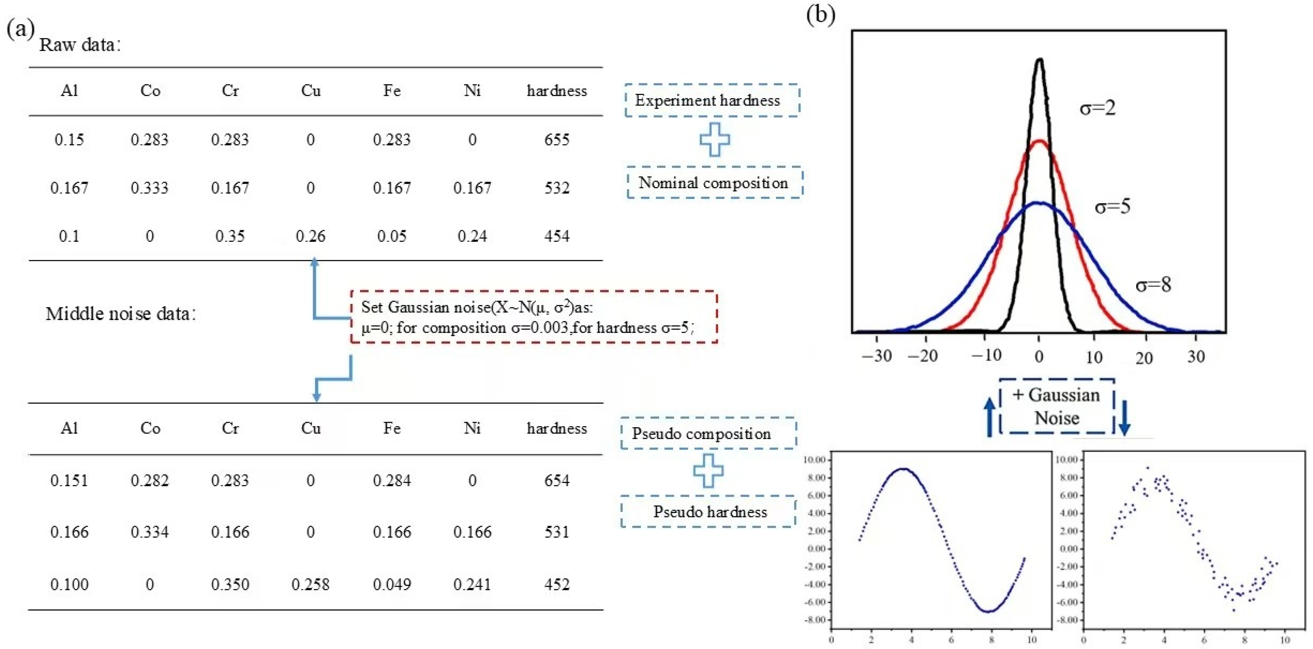
2.1. Gaussian Noise

Gaussian noise is a common type of noise, also known as normally distributed noise, which refers to adding random noise that follows a Gaussian distribution when processing the original data (Table S1). Material data have the same essence [15,16,21]. The nominal composition refers to the theoretical composition designed in the experiment, while the actual composition denotes the composition obtained through practical measurement during the preparation process. The inevitable weighing and preparation deviations in the preparation process were regarded as the inherent characteristics of material data. During the experimental process, there are inevitably deviations in the weighing and preparation of the alloys with the nominal composition designed, so the dataset is actually full of nominal compositions. Gaussian noise is adopted to simulate the composition deviations in the actual preparation process. By adding some noise to the nominal components, pseudo-samples can be obtained. In this method, the noise in the material data may be regarded as an inherent characteristic and further be utilized to generate “pseudo-data” containing noise. Then, the noise has been introduced into the model to expand the dataset and enhance the robustness of the model.

A schematic diagram of the process of adding Gaussian noise to the original data to obtain the “actual composition” is shown in Figure 1. Similarly, there are certain deviations in the hardness experiment. The hardness in the original dataset is the average value of multiple measurements, so noise also needs to be added to the output hardness. Therefore, a noise component with a standard deviation of σ = 0.003 and a noise hardness of σ = 5 HV is introduced into the original data. During the calculation process, a truncation method was employed to set negative values in the generated data to zero; thereby, unrealistic data was eliminated. Bayesian optimization was utilized for automatic parameter tuning to ensure that the generated data fell within a reasonable range. Figure 1a shows the comparison of the data before and after adding Gaussian noise to the hardness samples. Gaussian noise is a kind of random number, and its probability density function follows a Gaussian distribution. As can be seen from Figure 1b, the larger the value of σ, the more significant the effect caused by the noise. This method not only enables our model to better adapt to the changes and uncertainties in the real world, but it also effectively reduces the overly optimistic test results caused by the leakage of test data. In this way, by simply adding Gaussian noise to the samples, the dataset can be doubled.

It can be found that the introduction of Gaussian noise simulates the random fluctuations and measurement errors in the real environment, making the model more theoretically complete. In addition, the technique of using Gaussian noise for data augmentation has also expanded the sample data to a certain extent. The augmented dataset covers more combinations and variations, thus improving the model’s ability to capture the elemental composition of HEAs.

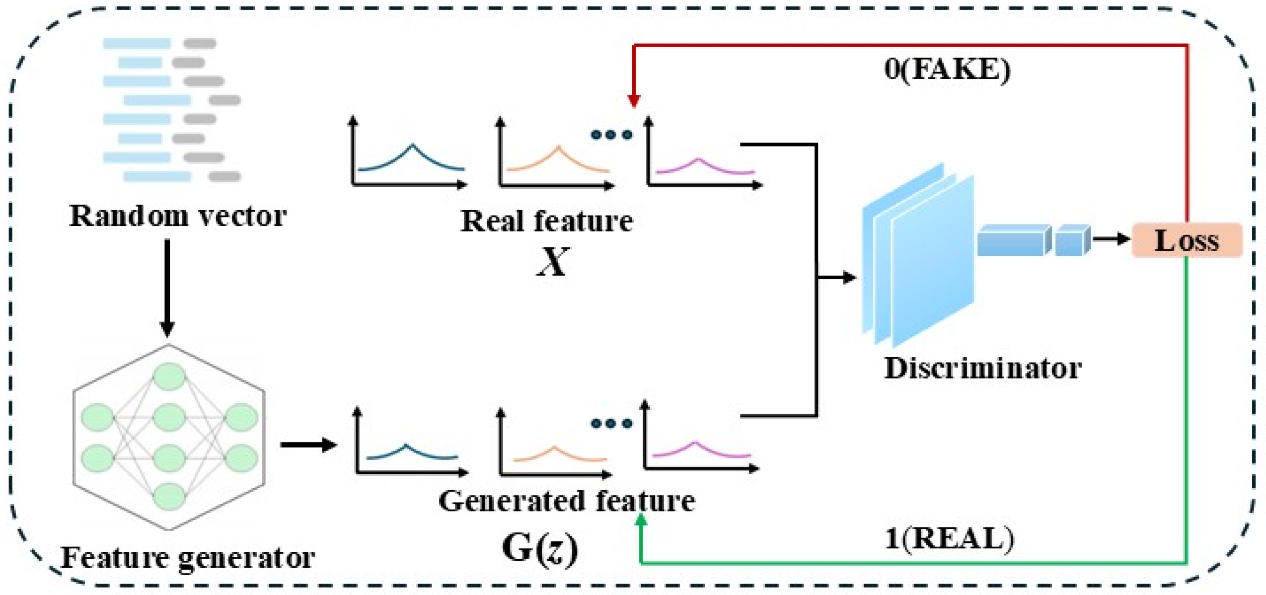
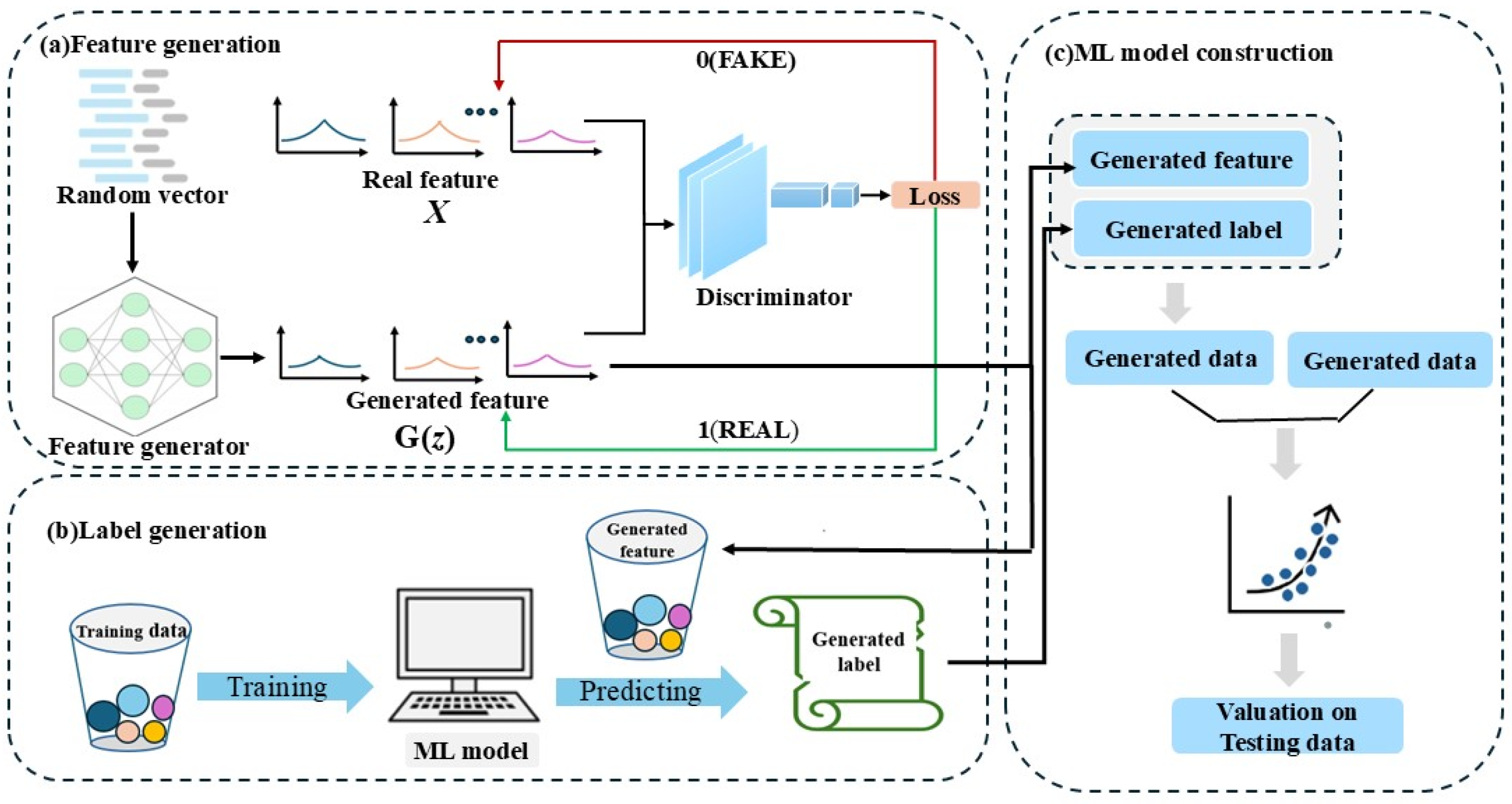
2.2. Generative Adversarial Network

2.2.1. Principle of GAN

In order to fully realize the improvement of the model’s prediction performance based on data augmentation, this project proposes the GAN and GANpro data augmentation methods and applies them to the research on the property prediction of HEAs. GAN originates from the zero-sum game in game theory, which is a non-cooperative game. In the game, the gain of one of the two participating parties will inevitably lead to the loss of the other party, resulting in the sum of the gains and losses of the two parties in the game always being zero. In GAN, there are two neural networks, namely the generator (generator, G) and the discriminator (discriminator, D). The discriminator D judges the samples generated by the generator G. The closer the data generated by the generator G are to the real data, the more difficult it is for the discriminator D to distinguish between true and false. In the early stage of training, the data generated by the generator G are of poor quality, so it is easy for the discriminator D to identify them as fake samples. However, during the training process, the generator G tries to generate data that are real enough to deceive the discriminator D, while the discriminator D tries to identify the true and false of each sample. In the process of the mutual game between the two, their respective generation ability and discrimination ability are continuously improved, and finally, the two parties reach an equilibrium point, which is called the Nash equilibrium.

The basic network structure of GANAs is shown in Figure 2. The generator G takes the random vector z that follows the standard normal distribution as the input and outputs the generated sample G(z). Then, the generated sample G(z) is put into the discriminator D for discrimination. If G(z) is closer to the real sample x, it is judged as 1. Otherwise, it is judged as 0.

Since the samples generated at the beginning of the training are difficult to be close to the real samples, the entire network needs to be continuously trained and optimized. The training of GAN is different from the previous single neural network. An alternating iterative training method is adopted, in which either the discriminator is optimized while the generator is fixed or the generator is optimized while the discriminator is fixed. The entire GAN can be unified into an objective function, which is shown in the following Formula (1):

$$\underset{\mathrm{G}}{\min }\underset{D}{\max }V\left(G,D\right)=E_{\mathrm{x}~Pd\left(\mathrm{x}\right)}\left[logD\left(x\right)\right]+E_{z~Pz\left(z\right)}\left[log\left(1-D\left(G\left(z\right)\right)\right)\right]$$

(1)

In Formula (1), x is a sample from the real data distribution Pd(x). z is a noise sample from the pre-defined random noise distribution Pd(x), and E is the expected value of the distribution function.

When the discriminator D is fixed and the generator G is optimized, the generated samples output by the generator G are judged as true or false by the discriminator D, and the discrimination loss is fed back to the generator G. The final result is that the generator can generate samples that can deceive the current discriminator D, and the discrimination result of the discriminator is close to 1. Therefore, the objective function for optimizing the generator is expressed as Formula (2):

$$\underset{G}{\min }V\left(G,D\right)=E_{\mathrm{z}~pz\left(z\right)}\left[\log \left(1-D\left(G\right)\right)\right]$$

(2)

When optimizing the discriminator D, the generator G is fixed. The discriminator improves its discrimination ability by continuously judging the real samples and the generated samples. The specific optimization function is shown in Formula (3):

$$\underset{D}{\max }V\left(G,D\right)=E_{\mathrm{x}~Pd\left(\mathrm{x}\right)}\left[logD\left(x\right)\right]+E_{z~Pz\left(z\right)}\left[log\left(1-D\left(G\left(z\right)\right)\right)\right]$$

(3)

A visualization of the GAN training process is shown in Figure 3. The equidistant points on the horizontal line z indicate that the data follow a uniform distribution. The arrow pointing from z to x represents that the random noise vector z is output by the generator G to generate the sample G(z). The green solid line represents the probability distribution of the generator, the black dotted line represents the probability distribution of the real data, and the blue dotted line represents the output of the discriminator. In Figure 3, there is a large difference between the probability distributions of the generated data and the real data. The output value of the discriminator (blue dotted line) is higher on the left and lower on the right, indicating that it can distinguish between true and false data well. With the increase in training, Figure 3 (after updating D) shows that by fixing G first and training D, the discrimination ability of the discriminator is improved. In Figure 3 (after updating G), by fixing D and training G with the information fed back by D, the distribution of the generated data approaches that of the real data. After multiple alternating trainings of D and G, the distribution of the generated data coincides well with that of the real data, as shown in Figure 3 (mixed strategy equilibrium). At this time, the discriminator can no longer distinguish between the generated data and the real data and guesses the truth or falsehood of the samples with a probability of 50%.

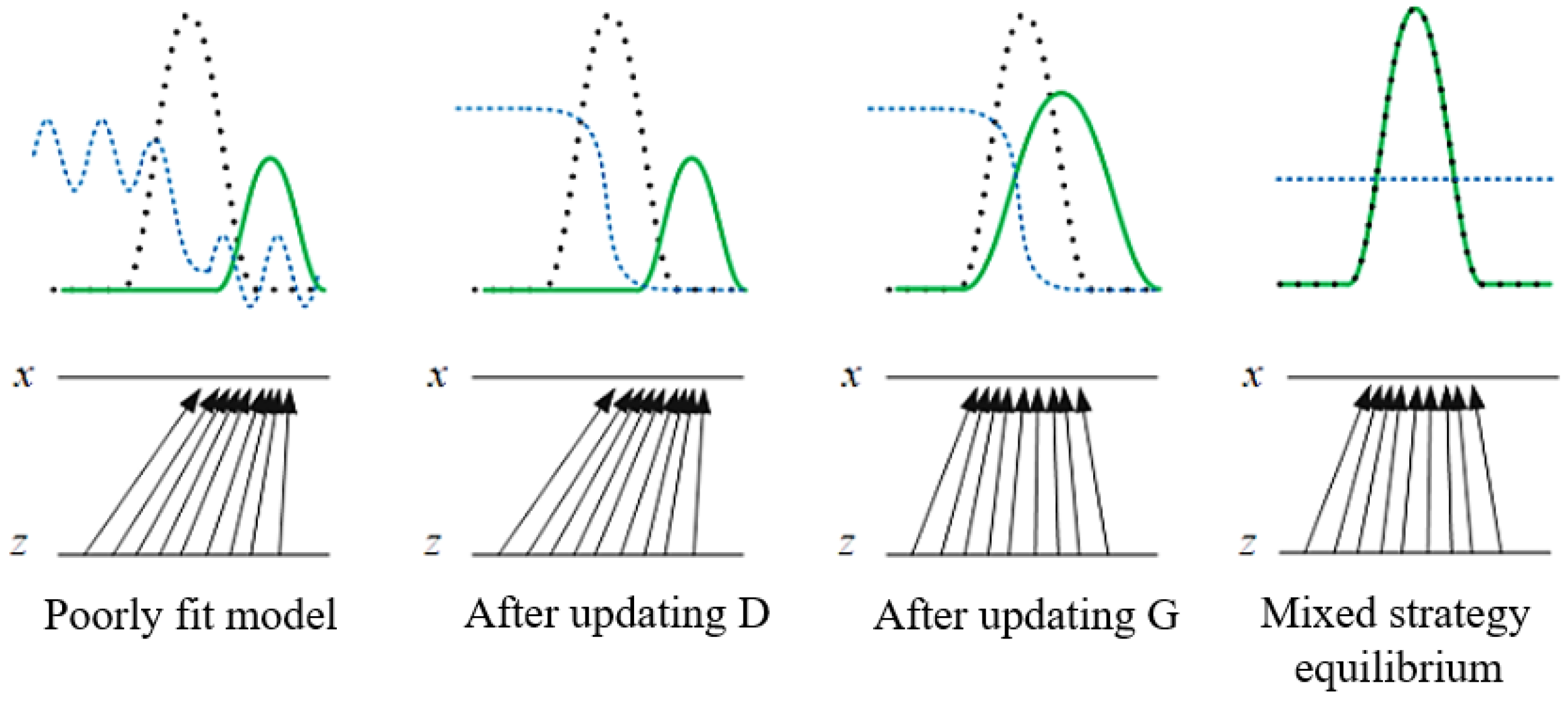
2.2.2. Principle of GANPro

In this project, based on GAN, a method for expanding data applicable to regression problems, namely the GANPro expansion method, is proposed, and the entire workflow of this method is shown in Figure 4. This method can perform data augmentation in regression tasks with a small number of training samples and improve the prediction model of the regression model by enhancing the quality of the features and labels of the generated data.

2.3. Machine Learning Evaluation Index

In the training of the regression model, the contents of six elemental components are selected as the input features, and the hardness is taken as the output label. Before the model training, the dataset should be normalized. For each feature shown in Formula (4), X_i replaces an original value, where X^min and X^max, respectively, replace the minimum and maximum values in this feature.

$$X_i^{norm}={\displaystyle \frac{X_i-X_i^{min}}{X_i^{max}-X_i^{min}}}$$

(4)

Different from the machine learning classification task, where only component noise is added, in the regression task, in addition to the component noise, noise also needs to be added to the hardness, which serves as the output. Moreover, since the output of the regression task is a continuous result, the change in data will have a more obvious impact. In this paper, the coefficient of determination (R2) shown in Formula (5) and the root mean square error (RMSE) shown in Formula (6) are selected as the evaluation criteria for the regression model. In Formulas (5) and (6), y_i is the true value in the dataset. $\overline{y}$ represents the average value of all y in the dataset, and $\widehat{yi}$ is the predicted value of the model.

$$\mathrm{R}2=1-{\displaystyle \frac{\sum {\left(y_i-{\widehat{y}}_i\right)}^2}{\sum {(y_i-{\overline{y}}_i)}^2}}$$

(5)

$$\mathrm{RMSE}=\sqrt{{\displaystyle \frac{1}{n}}{\sum }_{i=1}^n{\left(y_i-{\widehat{y}}_i\right)}^2}$$

(6)

3. Results

Referring to previous work, this study collected data on the HEAs of the AlxCoyCrzCuuFevNiw system from the literature [25,26,27]. Among them, x, y, z, u, v, and w are the molar fractions of each element, which are constrained by x + y + z + u + v + w = 100%. All alloy samples were prepared by vacuum arc melting, and their hardness was measured in the as-cast state. The original data information includes the composition of the alloy and the experimental hardness. Considering the data from different literature sources due to experimental equipment and error factors, alloy samples with the same composition but a large difference in the experimental hardness value were excluded when collecting data. For samples with a small difference in hardness, the average value was taken as the final hardness value. Finally, a hardness dataset of 205 AlCoCrCuFeNi alloy samples was obtained. The distribution of the alloy composition data is shown in Figure 5, in which the element Fe appears 201 times at the highest frequency.

In order to improve the generalization ability of the model and avoid overfitting, the 10-fold cross-validation method is adopted in this experiment to find the optimal hyperparameters. In addition, to reduce the impact of data leakage on the test accuracy, we have taken the following two key steps. Firstly, after integrating the noisy samples, the augmented data are randomly shuffled. Secondly, we divide the dataset into a validation set and a training set, which can also be regarded as a way of experimental verification.

The original data are analyzed, and the relationship between the content of each alloy element in the dataset and the hardness is shown in Figure 6. From the original dataset containing 205 hardness samples, 10% of the samples are retained as the validation set, that is, 21 hardness samples. The remaining 184 hardness samples are trained through 10-fold cross-validation. In this way, the data of the validation set will not be used during the training process, thus avoiding the inflated impact of data leakage on the accuracy of the test set. In order to simulate the possible composition deviation in the actual situation, we generate noisy samples by adding Gaussian noise to the composition content of the original samples. In the alloy experiment, this is equivalent to the variation introduced due to the deviation between the nominal composition and the actual composition during the weighing and preparation processes.

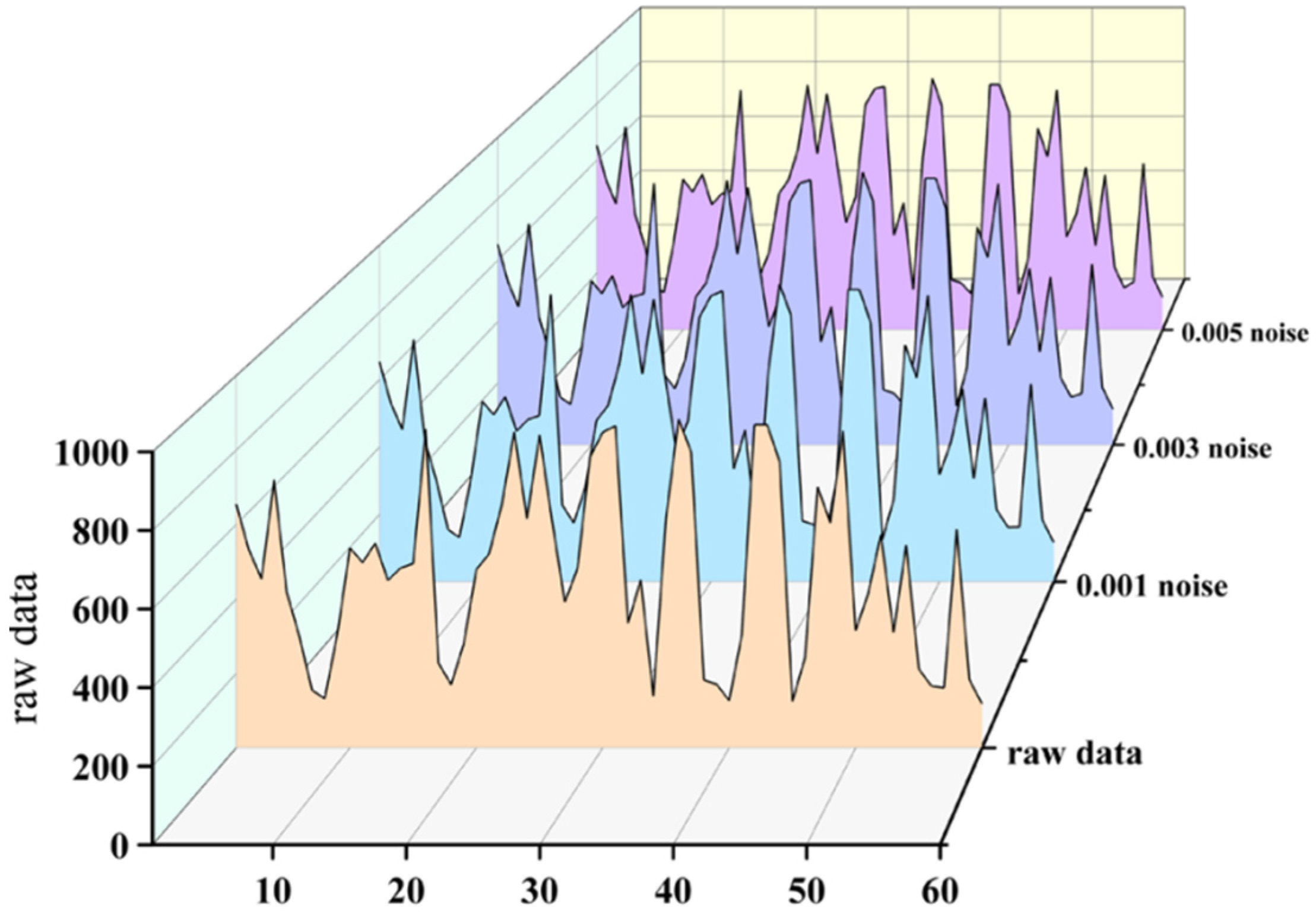
3.1. Enhancement and Expansion of the Alloy Dataset Using Gaussian Noise and Analysis of Performance Improvement

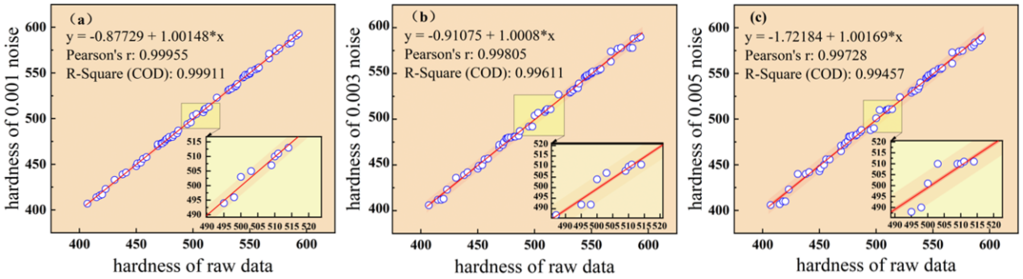
3.1.1. Analysis of Data Augmentation by Adding Different Noises

In the regression task, to enhance the sample augmentation effect, we add noise not only to the input features but also to the output hardness values. Since the results of the regression task are continuous, the impact of data changes on the model performance is more significant. Therefore, in this experiment, three different noise levels are set to increase the diversity of the data samples. Specifically, in this experiment, three noise components are considered, namely a low-noise component with σ = 0.001, a medium-noise component with σ = 0.003, and a high-noise component with σ = 0.005. In addition, according to the empirical fluctuations of the hardness of HEAs, a hardness with σ = 2 HV is regarded as low noise hardness, a hardness with σ = 5 HV is regarded as medium noise hardness, and a hardness with σ = 8 HV is regarded as high noise hardness. By adding these different levels of noise to the original data, a new augmented dataset is generated, as shown in

Table 1. Distribution of real and different noise data.

Materials	Raw Data	0.001 Noise	0.003 Noise	0.005 Noise
Al	0.2310	0.2314	0.2327	0.2339
Co	0.1540	0.1541	0.1548	0.1555
Cr	0.1540	0.1514	0.1466	0.1418
Cu	0.1540	0.1536	0.1532	0.1528
Fe	0.1540	0.1547	0.1565	0.1583
Ni	0.1540	0.1545	0.1559	0.1574
HV	498	496	497	488

.

Table 2. Means and standard deviations of real and generated data.

Number	Mean				Std
	Raw data	0.001 noise	0.003 noise	0.005 noise	Raw data	0.001 noise	0.003 noise	0.005 noise
1	0.2209	0.2207	0.2205	0.2203	0.1442	0.1442	0.1442	0.1442
2	0.1543	0.1544	0.1548	0.1547	0.0924	0.0924	0.0924	0.0925
3	0.1828	0.1828	0.1828	0.1829	0.0875	0.0874	0.0873	0.0874
4	0.0906	0.0906	0.0905	0.0904	0.0895	0.0895	0.0894	0.0894
5	0.1649	0.1648	0.1649	0.1650	0.0775	0.0776	0.0776	0.0778
6	0.1865	0.1865	0.1865	0.1866	0.1026	0.1024	0.1022	0.1020

and

Table 3. Maximum and minimum values of real and generated data.

Number	Min				Max
	Raw data	0.001 noise	0.003 noise	0.005 noise	Raw data	0.001 noise	0.003 noise	0.005 noise
1	0	0	0	0	0.470	0.472	0.476	0.480
2	0	0	0	0	0.333	0.428	0.429	0.430
3	0	0	0	0	0.317	0.554	0.551	0.549
4	0	0	0	0	0.225	0.290	0290	0.291
5	0	0	0	0	0.317	0.470	0.475	0.479
6	0	0	0	0	0.385	0.500	0.501	0.502

compare the statistical characteristics of real data and generated data, including means, standard deviations, minimums, and maximums, where Raw data denotes the real data, and Min and Max denote the generated data after adding different noises, respectively. From the three tables, it can be seen that the statistical characteristics of real data and generated data are well aligned. Here, the quality of features in the generated data is only evaluated with statistical metrics; the quality of labels should not be simply measured with statistical metrics, but the generated data should be added to the training set to retrain the model and evaluated based on the prediction performance of the new model.

Sixty sets of sample data were randomly selected, and 3D waterfall plots were drawn to show the data distribution under different noise conditions. As shown in Figure 7, it can be clearly seen from the graph that the data distribution after adding different degrees of noise is basically the same as the fluctuation of the original data. This indicates that the overall trend and characteristics of the data remain stable even with the introduction of noise, which does not cause significant shifts or distortions in the data. Specifically, the fluctuations of the 0.001 low-noise, 0.003 medium-noise, and 0.005 high-noise samples in all dimensions do not significantly deviate from the distribution of the original data, which verifies the reasonableness and validity of our noise addition method.

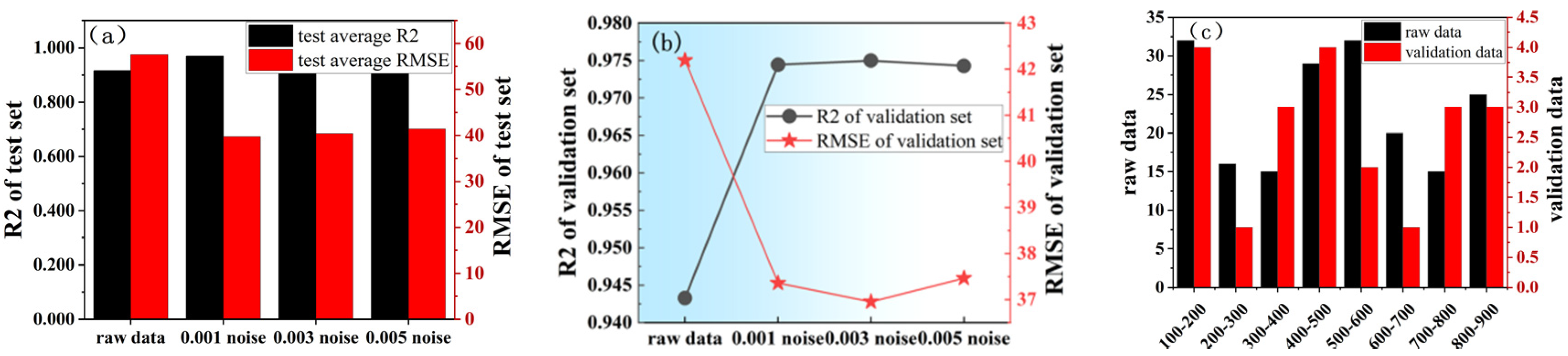
3.1.2. Effect of Different Noise on Model Performance

By further adding different noise samples to the original data, the results of the study show that the new dataset enhanced with noise samples can make the model perform better. The new dataset, containing the original data and the enhanced data with different noise levels, was used in the experiments. The histograms in Figure 8 show the accuracy of the models based on different enhanced datasets on the test set. Specifically, the following four datasets are included in the figure: a dataset containing only the original data, a dataset containing the original data and 0.001 noise low-noise samples, a dataset containing the original data and 0.003 noise medium-noise samples, and a dataset containing the original data and 0.005 noise high-noise samples. In Figure 8a, the black bars on the left axis are the test set R2 averages, and the red bars on the right axis are the RMSE averages. The RMSE is more sensitive to having larger values for the error; so, for example, the RMSE of the three models enhanced with noise samples is lower than that of the initial model. The RMSE of the four augmented models have smaller relative errors, and the accuracy of the three models based on augmented data has been improved to some extent compared with using only the original data. In addition, it can be seen from the change in R2 that the augmented dataset helps improve the predictive ability of the models, which makes the models perform better on the test set. These results show that the noise sample enhancement technique not only effectively expands the dataset but also significantly improves the prediction accuracy and robustness of the models, confirming that the sample-enhanced models have a better fit and provide a more reliable technical means for the prediction of the properties of HEAs.

Although it is a random process for data reading and processing, noisy data is not actually the same as the original data. Therefore, validation data that the model has never seen before is needed. The line graphs in Figure 8b show the R2 and RMSE of the model based on different augmented datasets on the validation dataset. The experimental results show that the test accuracy of the model is significantly improved by adding noisy samples. In particular, the introduction of medium- and high-noise samples enables the model to better capture complex patterns in the data, which improves the prediction performance. Among them, the 0.003 medium-noise-enhanced model has the highest R2 (0.974) and the lowest RMSE (36.952). This suggests that data enhancement by adding different levels of noise samples in the regression task can indeed effectively improve the performance of the model, resulting in greater robustness and higher prediction accuracy for brand-new data.

To further eliminate tendencies in data selection, we compared the distributions of the original and validation data. Specifically, we statistically analyzed the hardness values of the original and validation datasets and plotted histograms of their distributions. As shown in Figure 8c, the hardness distribution of the validation set is almost similar to that of the original data at every interval. This indicates that we did not introduce any obvious bias in the selection of the validation dataset, ensuring the reliability and representativeness of the validation results.

As shown in Figure 9a–c, sample data with hardness values in the range of 400–600 are selected, and the confidence intervals of the samples with different levels of noise added are plotted, respectively, from which it can be seen that the fluctuation ranges of the sample data change significantly with the increase in the degree of noise, but the overall trend is still consistent with the original data. Figure 9 clearly demonstrates the impact of different noise levels on the sample data, further verifying the robustness of the model under different noise conditions.

Then, the effect of adding more noise-enhanced data on the model was further tested, as shown in Figure 10. Where 2 × R represents that the raw data is enhanced twice. L represents low-noise data, M represents medium-noise, and H represents high-noise enhancement. In addition, 3 × R represents that the raw data is enhanced twice. L + M represents raw data, low-noise data, and medium-noise data. L + H represents raw data, low-noise data, and high-noise data. M + H represents raw data, medium-noise data, and high-noise data. Also, 4 × R represents that the raw data is enhanced three times. L + M + H represents raw data, low-noise data, medium-noise data, and high-noise data.

As can be seen from Figure 10, showing the test RMSE and validation RMSE of the model with different data, it can be found that the test RMSE decreases instead with the increase in data, indicating that the model is well fitted. However, the validation RMSE shows an overall increasing trend with increasing data, indicating that the generalization ability of the model is decreasing. The high fit and generalization ability of the model prove that the model is overfitted. This is due to the fact that noisy data is generated from the original data, and adding too much is bound to lead to data leakage problems. Adding more data only improves the fit of the model but does not have much impact on improving the generalization ability of the model. Overall, noise sample enhancement can only be used once.

3.2. Enhancement and Expansion of the Alloy Dataset Using Generative Adversarial Networks (GAN) and Its Performance Improvement Analysis

In order to test its performance, in this experiment, the same 205 HEAs’ hardness values with Gaussian noise were still used, and after the steps of feature construction, feature selection, model evaluation, and parameter optimization, the original model with excellent performance was trained. Then, on this basis, the effectiveness of the GAN and GANpro expansion methods is evaluated, and the effect of different sample numbers of generated data on model performance improvement is explored. Finally, the generalization ability of the new model after data augmentation is evaluated on 18 alloy samples independent of the training dataset. The results show that the GANpro expansion method proposed in this paper can effectively alleviate the data shortage problem in the HEA regression problem and provide a demonstration of application potential under the specific conditions for HEA performance prediction and composition design studies. This is consistent with the machine learning method based on GAN and NN proposed by Roy et al. [28] for the efficient design of high-hardness multi-principal element alloys (MPEAs). They autonomously generated new alloys in the composition space containing 18 elements through GAN and used the NN model to screen out candidate materials with significantly improved hardness. The hardness of the optimal composition (Co-Fe-Ni-Al-Cr-Mo-Ti system) reached 941 HV, which was 10% higher than the highest value (857 HV) in the training data, breaking through the composition limitations of the traditional Al-Co-Cr-Fe-Ni system. Looking at the feature importance analysis from the visualization point of view, as shown in Figure 11a, it is easy to intuitively find the important role of Al and Ni. Here, the average scores of the input features are given using different machine learning algorithms to give their respective feature importance scores, which are then ranked according to the average importance score of each feature. These algorithms include Linear Base Kernel Support Vector Machine (SVR.linear), Random Forest (RF), Extreme Gradient Boosting Tree (XGboost), Linear Regression, and Ridge Regression. Too many feature dimensions may contain repetitive or redundant information, which can easily cause the overfitting of the machine learning model and affect the prediction performance and generalization ability. Therefore, using compositional information as feature input can explain the prediction results of the model more easily, and it is possible to intuitively understand how the increase or decrease in a certain element affects the hardness of the alloy, and its related heat map is shown in Figure 11b. We can clearly see the relationship between different element contents and alloy hardness. The thermogram demonstrates the correlation between the elemental content and the hardness value, and the strength and direction of this relationship are shown by the change in colour. This visual representation allows us to quickly understand the trend of how an increase or decrease in an element affects the hardness of an alloy.

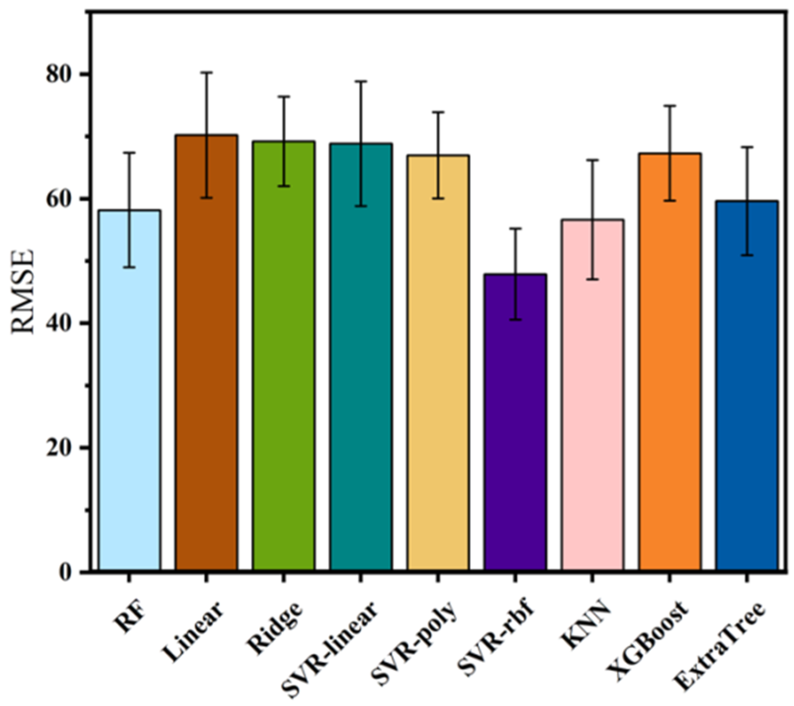
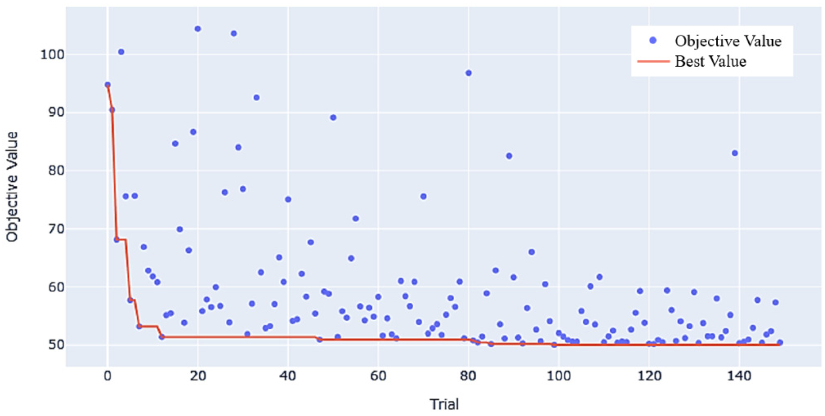
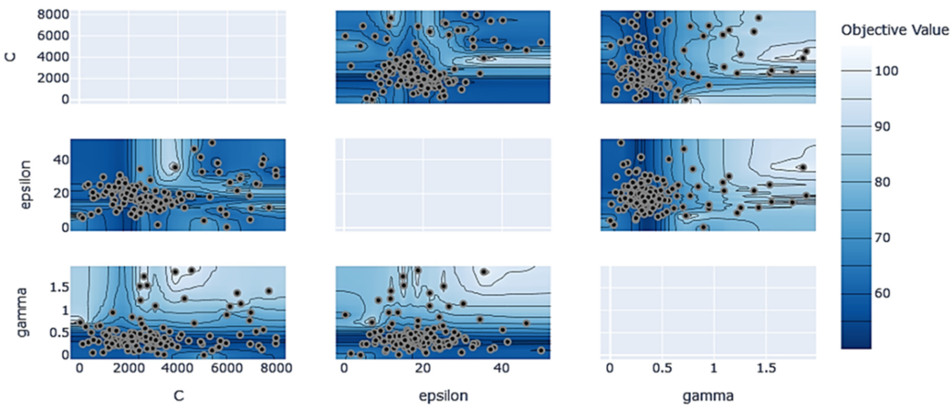
3.2.1. Evaluation of Different Algorithm Modelling

Next, we evaluated nine different types of machine learning algorithms, including Linear, Ridge, Linear Kernel Support Vector Machines (SVR-linear), Polynomial Kernel Support Vector Machines (SVR-poly), Radial Basis Kernel Support Vector Machines (SVR-rbf), Nearest Neighbour Model (KNN), Random Forest (RF), Extreme Gradient Boosted Tree (XGBoost), and ExtremeTree. All of these algorithms use six elemental components as inputs to build corresponding machine learning models to evaluate the performance of each model, and RMSE and R2, which have large error fluctuations, are chosen as the criteria for the error evaluation of the regression models. In the model evaluation process, the dataset is divided into a 90% training set and a 10% test set. In order to eliminate the randomness associated with a single dataset division and to perform hyperparameter optimization, 10-fold cross-validation was used; 10-fold cross-validation is a commonly used evaluation method, which is performed by dividing the dataset into 10 mutually exclusive subsets, and each time, one of the subsets is used as the validation set, and the remaining subset is used as the training set. This is carried out 10 times to ensure that each subset is used as a validation set once, and finally, the average of all validation results is taken as the basis of model performance evaluation. This method can effectively reduce the impact of randomness due to a single dataset division and ensure the reliability and stability of the model evaluation results. By comparing the performance of different algorithms, we are able to identify the model with the best performance on the HEAs dataset, which guides the choice of the most suitable algorithm in practical applications, as shown in

Table 4. Description of the regression algorithm.

Algorithm	RF	Linear	Ridge	SVR-Linear	SVR-Poly	SVR-rbf	KNN	XGBoost
R2(100%)	92.1	87.3	90.6	90.8	92.6	96.4	93.6	90.2

.

The RMSE and error bar results under different models are shown in Figure 12. The evaluation results show that different algorithms have different performances when dealing with the same dataset, and it can be seen that the linear model Linear performs the worst, which indicates that the relationship between the six component features and the hardness is not just a simple linear relationship, and a more complex model is needed to map the relationship between the features and the mapping. The prediction results of the three models, Ridge, SVR-linear, and SVR-poly, are also not ideal. The SVR-rbf model performed the best, which is also in line with the best models obtained from several studies that are suitable for the hardness prediction of HEAs. In addition, the same model selection results can be obtained by evaluating the best performance index of SVR-rbf model based on the regression coefficients.

The setting of hyperparameters of machine learning models is crucial to model performance, and this subsection takes the SVR-rbf model as an example to illustrate the optimization of model hyperparameters during the establishment of a high-entropy alloy hardness prediction model. Compared with the traditional grid search and random grid search methods, Bayesian optimization is able to use the previous historical results in the search process to guide the selection of hyperparameters in the next search, so Bayesian optimization methods are used to find the best combination of hyperparameters for the high-entropy alloy hardness model. The 10-fold cross-validation method is used to evaluate the method to optimize the hyperparameters. I.e., the objective value of Bayesian optimization is the average error of the 10-fold cross-validation; the hyperparameters to be optimized for the SVR-rbf model are C, epsilon, and gamma; the search ranges of the three important parameters are (1, 8000), (1, 30), and (0.0001, 2); and the other parameters are all chosen as the default values for all other parameters. Figure 13 shows the trend of the objective function value during 150 searches, and it can be seen that the error curve of the minimum value is basically unchanged after gradually decreasing from a high value, which indicates that 150 searches are sufficient for the current model, and it also shows that the Bayesian optimization will refer to the historical search results to give the hyperparameters of the next search, so that the value of the objective function is steadily improved with the number of searches.

In addition, a contour plot of the variation in the objective values during the hyperparameter optimization process is given in Figure 14, showing the variation in the three hyperparameters with respect to the value of the objective function during the hyperparameter search process. It can be seen that the optimal hyperparameters corresponding to the SVR-rbf model for HEAs’ hardness prediction are in the range of approximately 2136 for C, 15 for epsilon, and 0.3 for gamma, which will provide the parameter ranges for our subsequent fine-tuning of the model. The results of the hyperparameter visualization provide more detail on the optimization process and allow us to understand the model itself better.

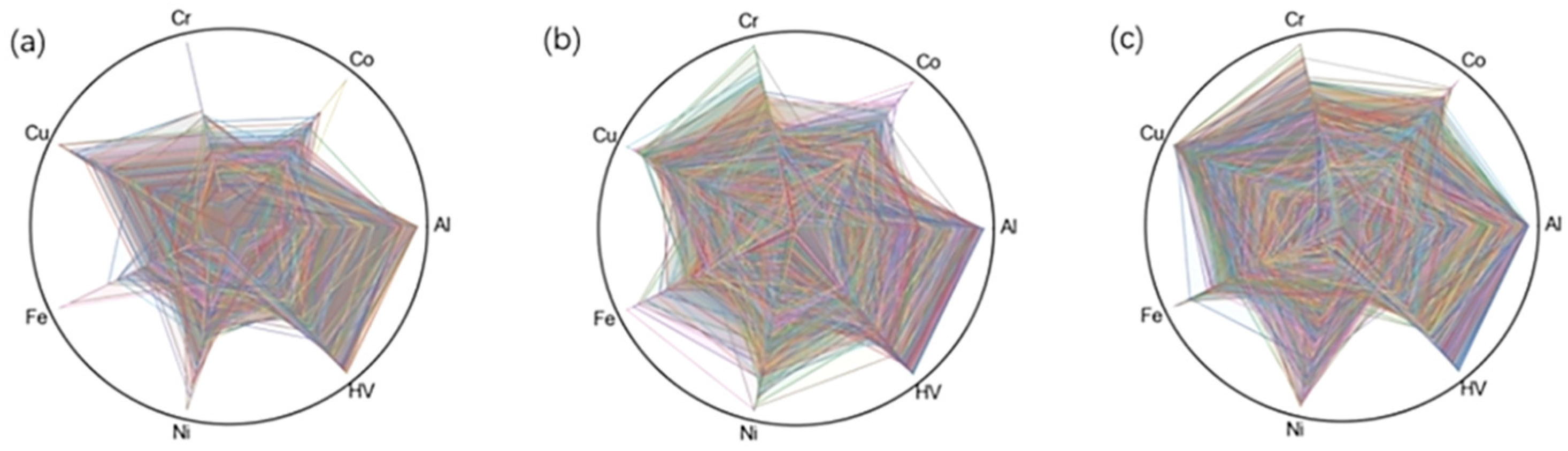
3.2.2. Distribution of Generated Data

The premise that the GANpro expansion method can improve the prediction accuracy of the model is that the first step is to generate generated data with the same distribution as the real data to achieve the purpose of expanding the samples of the training set, and the key lies in the quality of the generated data features and labels.

Table 5. GAN structure of GANPro expansion method in HEAs hardness prediction.

Generator Network			Discriminator Network
Layer	Type	Dimension	Layer	Type	Dimension
Input	Latent	10	Input	Latent	6
Hidden1	Dense layer	128	Hidden1	Dense layer	128
	Batch normalization			Batch normalization
	LeakyRelu			LeakyRelu
	Dense layer	64		Dense layer	64
Hidden2	Batch normalization		Hidden2	Batch normalization
	LeakyRelu			LeakyRelu
	Dense layer	32		Dense layer	32
Hidden3	Batch normalization		Hidden3	Batch normalization
	LeakyRelu			LeakyRelu
output	Dense layer	6	output	Dense layer	7
	Tanh activation			Tanh activation

summarizes the network structure of the GAN in the GANPro method for HEAs hardness prediction.

In order to evaluate the ability of the GANpro expansion method in simulating the real data distribution and generating data with the same distribution, the real features of the training set are fed into the GAN training. Then, 400 features of the generated data are generated by sampling from the learned distribution, and then the generated features are predicted to achieve the generated labels with the best model obtained based on the training set; in this way, we obtain the generated data based on the GANpro expansion method. As a comparison, the features and labels of the same training data are directly obtained by inputting the features and labels of the generated data into the GAN together. As shown in Figure 15, the distributions of features and labels for the 400 pieces of generated sample data are shown in the form of radar charts, respectively, to visualize the distribution trend of the whole dataset in each dimension in general by representing the values of all dimensions comprehensively on the polar axes, where Figure 15a is the original sample data, Figure 15b is the sample data generated under the GAN method, and Figure 15c is the sample data generated under the GANpro method. It can be seen that the features of the data generated by either the ordinary GAN or GANpro expansion method are extremely similar to the real features of the training set, indicating that, in terms of generating features, the two data expansion methods can realistically simulate the distribution of features in the training set.

Table 6. Means and standard deviations of raw and generated data.

Number	Mean			Std
	Raw	GAN	GANpro	Raw	GAN	GANpro
1	0.221	0.222	0.223	0.001	0.062	0.226
2	0.153	0.152	0.149	0.148	0.019	0.019
3	0.185	0.175	0.183	0.058	0.029	0.010
4	0.091	0.089	0.089	0.129	0.014	0.188
5	0.164	0.160	0.165	0.058	0.012	0.131
6	0.185	0.185	0.185	0.097	0.037	0.085

and

Table 7. Maximum and minimum values for raw and generated data.

Number	Min			Max
	Raw	GAN	GANpro	Raw	GAN	GANpro
1	0	0	0	0.470	0.049	0.469
2	0	0	0	0.429	0.338	0.409
3	0	0	0	0.556	0.501	0.551
4	0	0	0	0.290	0.272	0288
5	0	0	0	0.469	0.407	0.422
6	0	0	0	0.500	0.471	0.498

compare the statistical characteristics of raw data and generated data, including means, standard deviations, minimums, and maximums, where Raw denotes the raw data and GAN and GANpro denote the GAN method and GANpro expansion method, respectively. As can be seen from Table 6 and Table 7, the statistical features of the raw and generated data are well aligned. Here, only the quality of features in the generated data is evaluated with statistical metrics, and the generated data is subsequently added to the training set to retrain the model and evaluated based on the prediction performance of the new model.

In summary, both the GANpro expansion method and the ordinary GAN are able to generate additional generative data from raw data, and the difference between the two lies in their different ways of handling the labels in the generative data. The former is to predict the generative features based on the best model of the raw data, in order to achieve the generative labels. This different process allows GANpro to potentially have some advantages in generating high-quality labels, especially when the label information is more complex or the data distribution is not uniform. The latter, on the other hand, uses the label information as a dimension of the GAN input and generates features and labels directly through GAN training. In this aspect of feature generation, there is no essential difference between the two, so both are able to generate features that are consistent with the distribution in the real data very well.

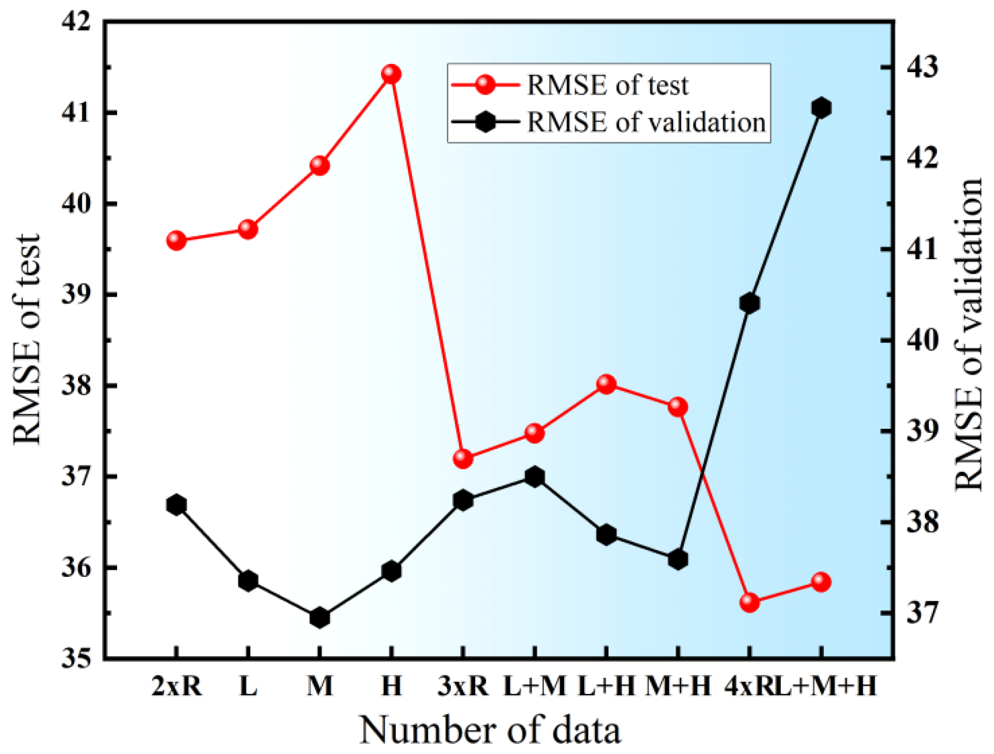
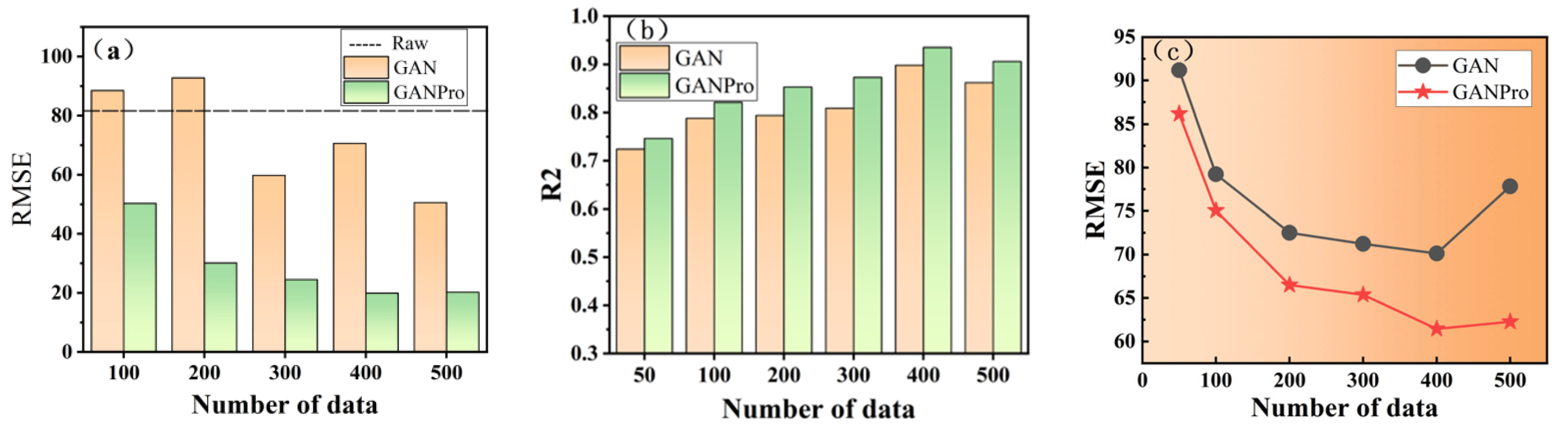
3.2.3. Impact of the Amount of Generated Data on Model Performance

Visualizing the feature distribution through radar distribution plots has demonstrated that both the GANpro expansion method and plain GAN can generate features well. On the other hand, in order to explore the impact of data augmentation methods on model performance under different generated dataset sizes, different amounts of generated data are added to the training set to retrain the model, the impact of the generated data on model performance is evaluated in the same test set, and the two data augmentation methods are compared. Specifically, the dataset was randomly separated 10 times; each time, 90% of the dataset was taken as the training set and 10% as the test set, different amounts of generated data were generated from the training set, and the RMSE of the model was evaluated in the same test set under the premise of fairness. Finally, the average of the 10 results was taken for the evaluation in order to avoid the randomness generated by randomly dividing the dataset. Test errors of the three models with different numbers of generated data are shown in Figure 16. In Figure 16a, the black dashed line in the figure indicates the best model obtained by training with the real training set, and the orange and green bar distributions indicate the new models obtained by the ordinary GAN method and the GANPro expansion method. The results show that for GANPro, the number of generated data significantly affects the prediction of the model, and the average error of the model shows a general trend of decreasing and then increasing with the number of generated data and exhibits the minimum error when 400 generated data are added. This is because when the number of generated data is small, the additional information provided by the expanded data is limited, whereas if the number of generated data is too large, this tends to bring in redundant and irrelevant information, making the model overfitted, and the same conclusion can be obtained in the GAN model as a whole. In addition, the figure further shows that GANPro significantly outperforms GAN, and both outperform Raw, which is another proof that data augmentation for GAN is beneficial to improve model performance. In addition, Figure 16b shows the R2 generated under different algebraic models. This figure further shows that GANPro significantly outperforms model-1, and both outperform GAN, which is another proof that the data augmentation of the GAN method is beneficial to enhance the model performance. In order to further compare the quality of the generated data produced by the GANPro expansion method and the normal GAN method, we trained the machine learning models on the generated data only. That is, under the condition of removing the raw data from the training set, GAN and GANPro were retrained again, and the calculated error average results for different numbers of generated data are shown in Figure 16c.

3.3. Comparison Between Gaussian Noise and Generative Adversarial Network in Regression Data Augmentation

In the field of data augmentation for regression-type machine learning tasks, Gaussian noise injection and Generative Adversarial Networks, as two typical data augmentation strategies, exhibit significant performance differentiation characteristics. Through systematic experimental comparisons, this study has found that although both methods are significantly superior to the original dataset in terms of data augmentation effect (p < 0.01), there are essential differences in their mechanisms of action and applicable scenarios. Gaussian noise augmentation has the advantage of linear time complexity by injecting random perturbations that conform to the normal distribution into the feature space. This parameterized augmentation method shows good computational economy in scenarios with scarce data (n < 10³), especially for medium- and low-dimensional regression problems with a feature dimension d ≤ 10, and it can effectively alleviate the overfitting tendency of the model. In the GAN framework, the generator G and the discriminator D are trained through the minimax game. This adversarial training mechanism enables the generator to learn the latent distribution characteristics of the data manifold. Theoretical studies have shown that when the Nash equilibrium condition is satisfied, this characteristic enables it to exhibit stronger distribution approximation ability in high-dimensional nonlinear regression problems (d > 10).

Although GAN theoretically has a better distribution modelling ability, the regression task experiment of this project, based on the AlCoCrCuFeNi HEAs dataset, shows in the RMSE and R2 indicators that the Gaussian noise augmentation method has a relatively higher improvement in the prediction accuracy of the test set, and the accuracy reaches 97.4% under medium noise. Gaussian noise in the low-dimensional feature space is sufficient to simulate the perturbation pattern, while it is difficult to train a stable GAN with a small sample size. Follow-up research will explore (1) the critical points of different dimensional noise methods and (2) a hybrid noise scheme combining GAN generation and Gaussian perturbation.

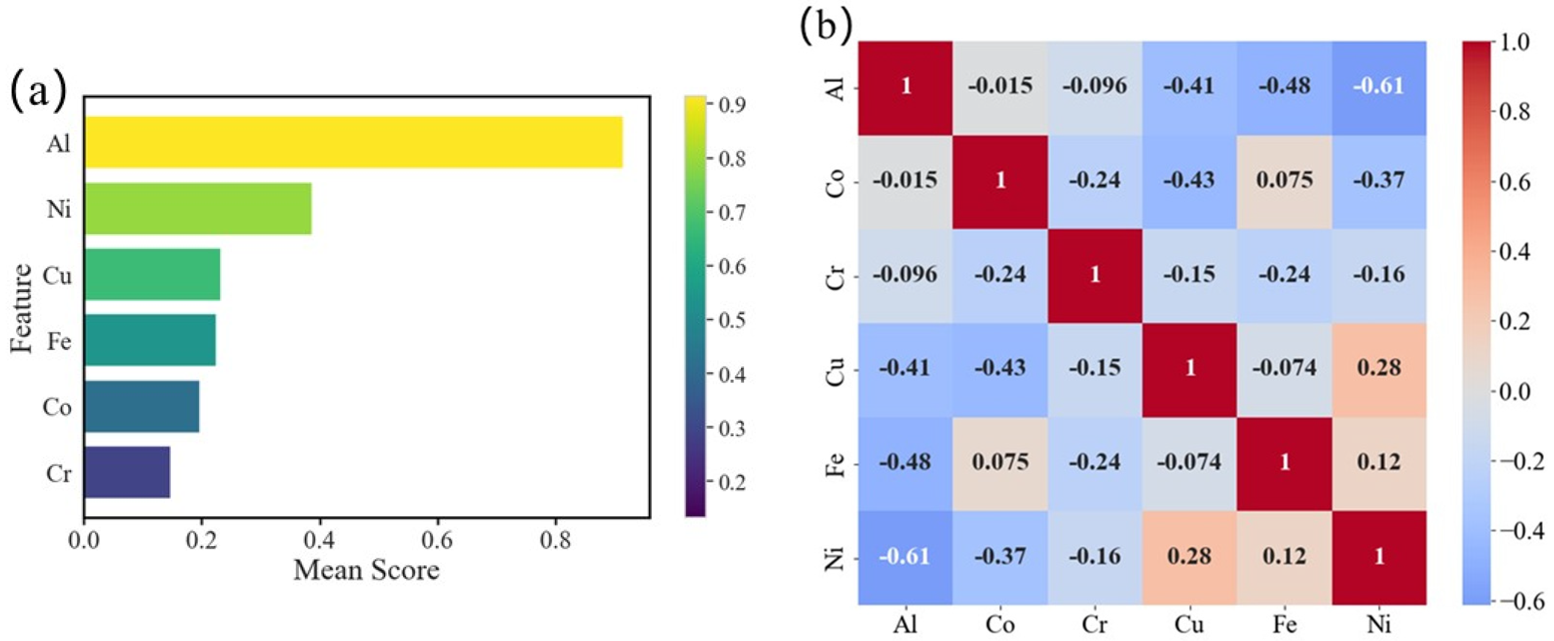
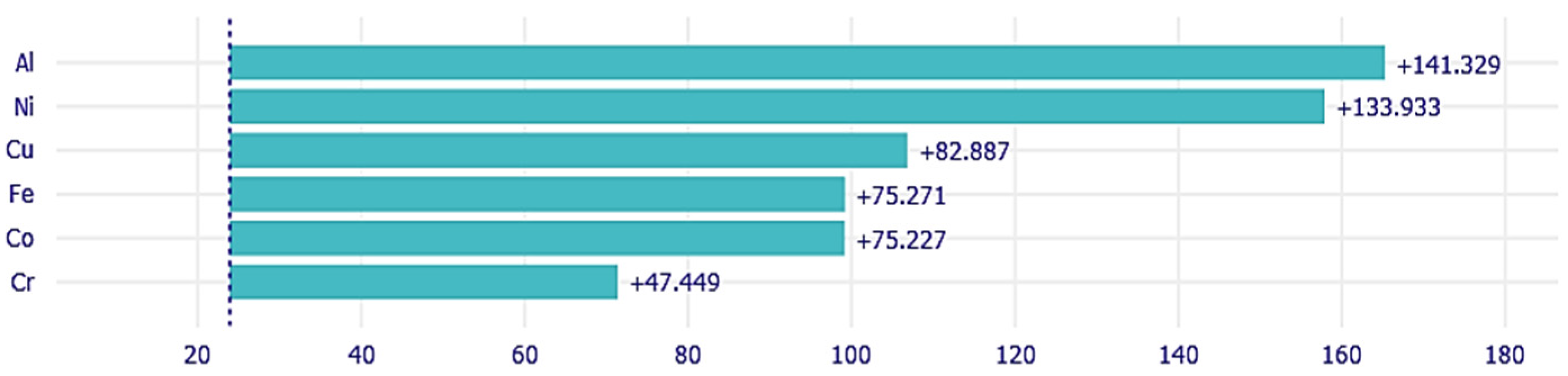
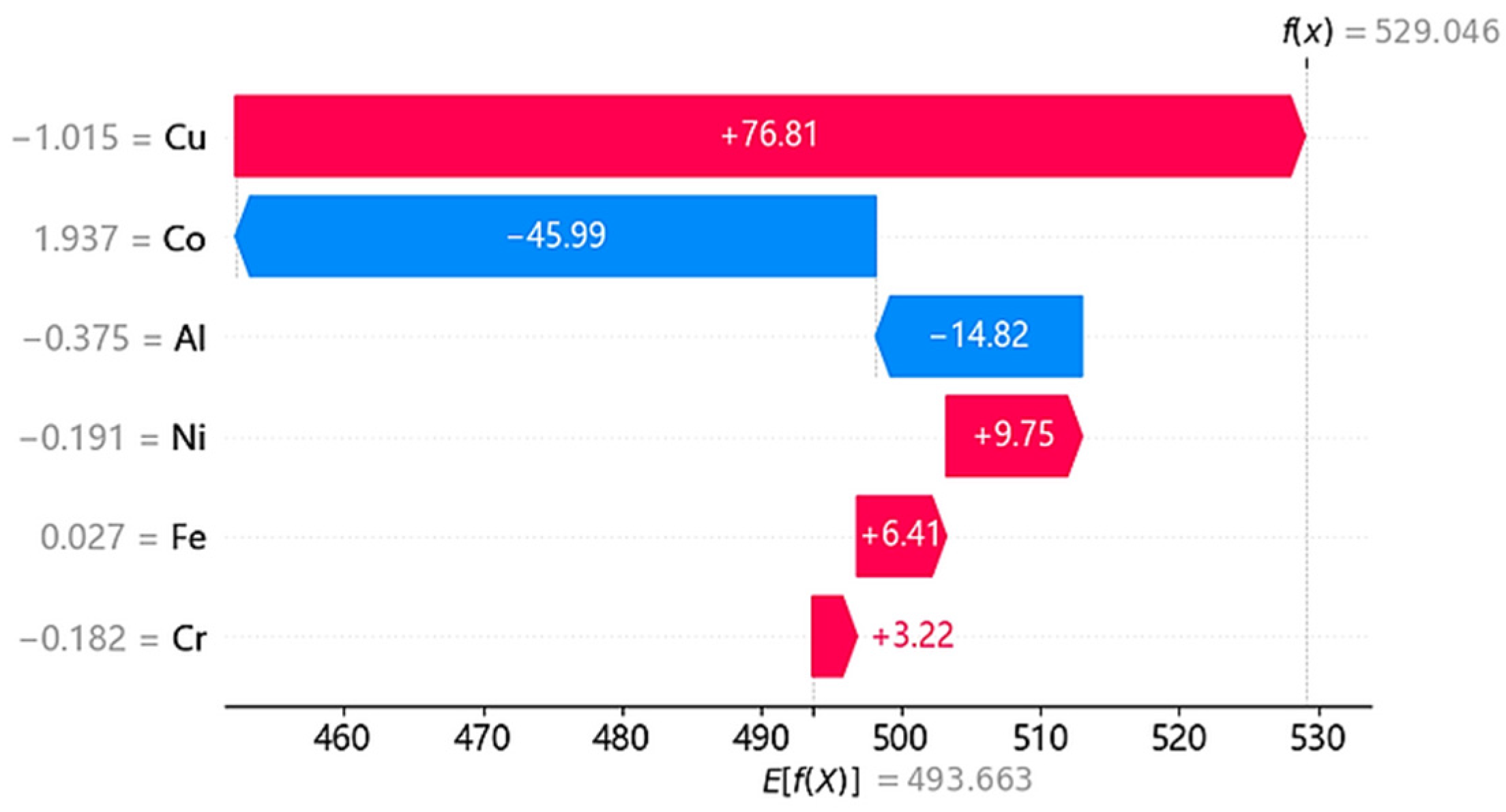
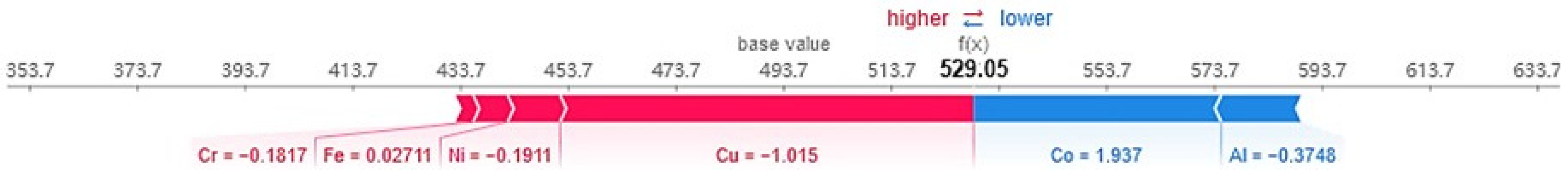
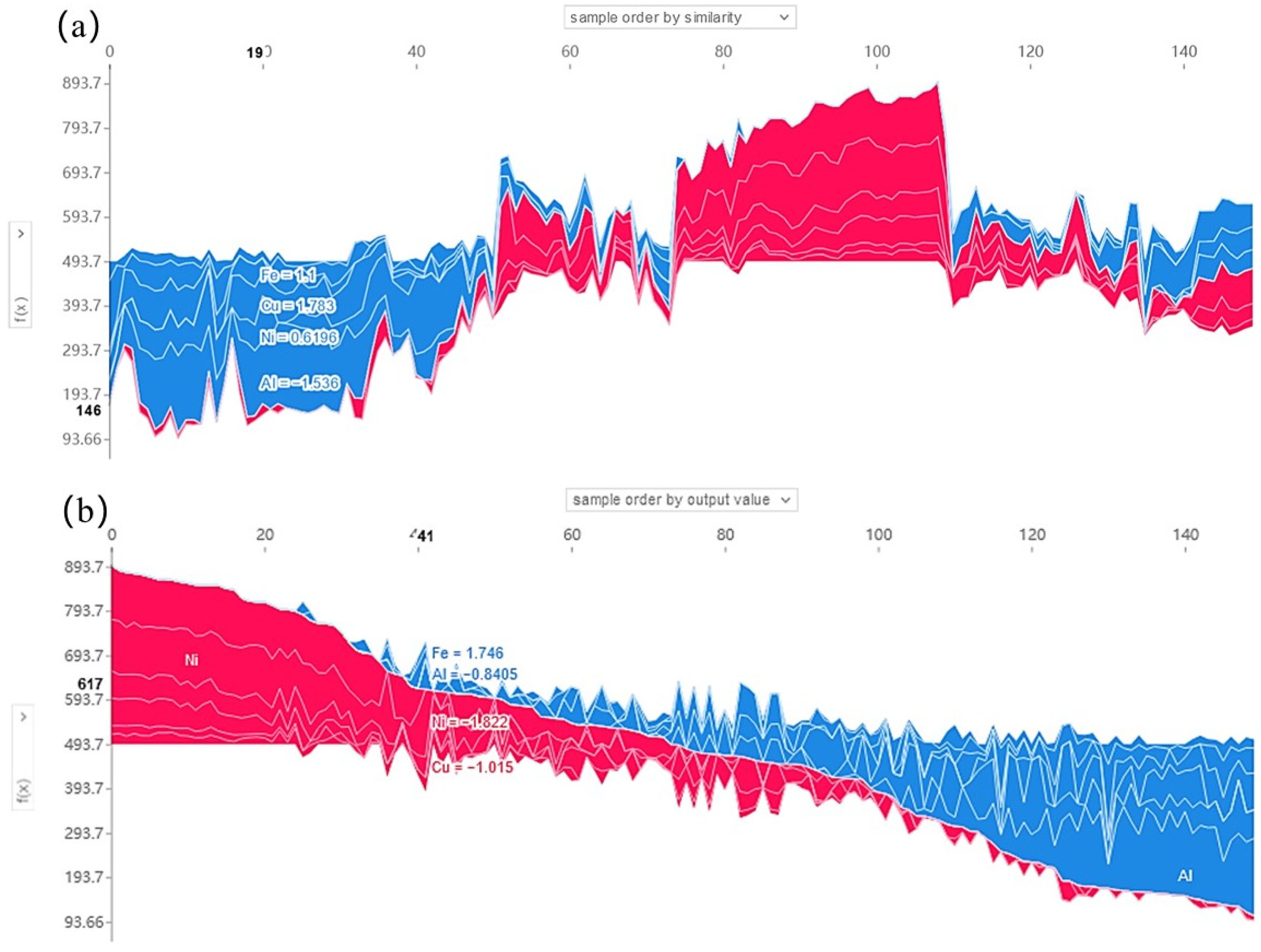
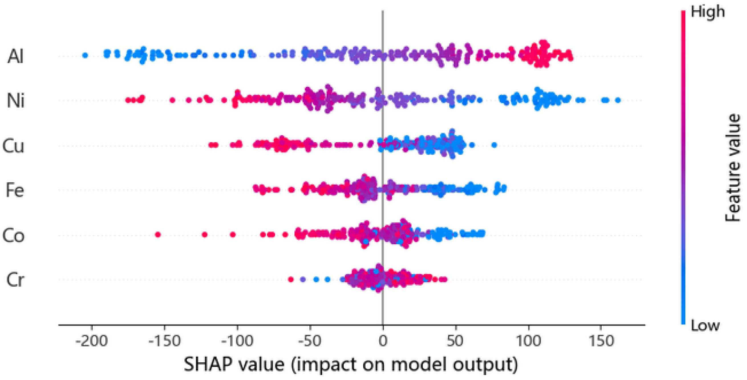
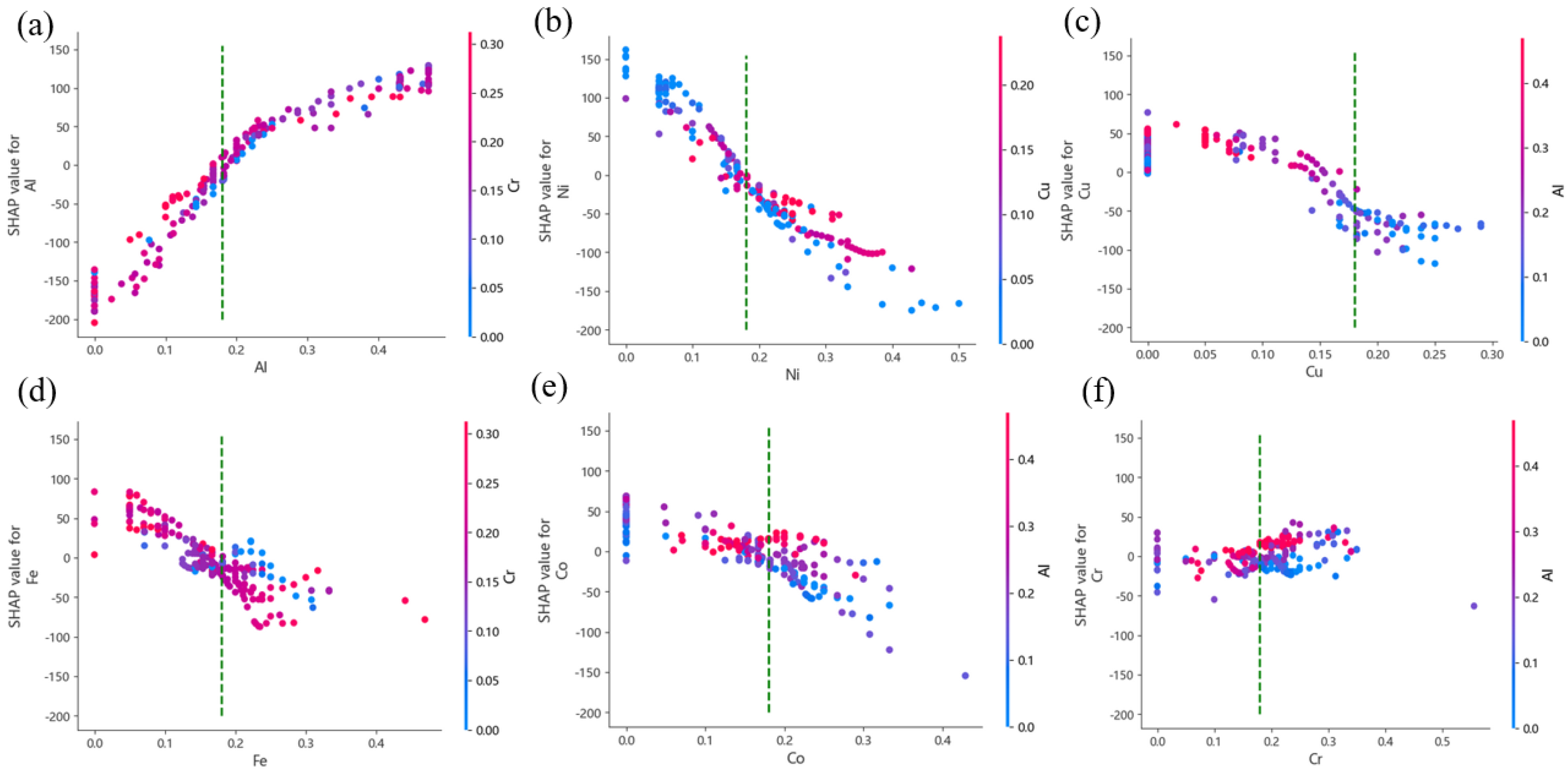
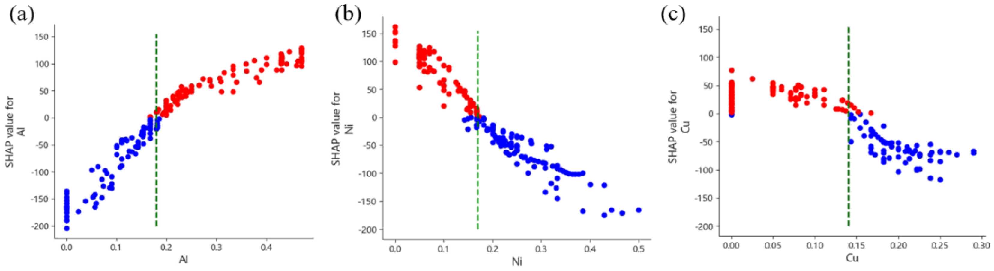
3.4. Interpretability Analysis of HEAs’ Hardness Prediction

In this experiment, two interpretability methods, including feature importance and the SHAP interpretation method (Shapley Additive Explanations) [28], are applied to the previously established HEA hardness prediction model for interpretability analysis. The outputs of these interpretive methods can help us understand the basis on which the model makes prediction decisions, providing the importance of features to the model’s prediction and the influence of different feature values on the prediction results.

The permutation importance method and the SHAP method are used to obtain the global and local importance of the model. Global importance is used to understand how the model makes predictions based on the overall understanding of the model, while local feature importance is based on how each feature affects the prediction result of a single sample. These methods do not make any assumptions about the model structure, so they can be applied to any prediction model. First, the permutation importance method is used to evaluate the importance of each feature in terms of the overall prediction performance. Specifically, after obtaining the trained SVR—rbf model, the values of each column of features are shuffled in turn while keeping the data in other columns unchanged, and predictions are made on the resulting dataset. If the model is highly dependent on the randomly shuffled column of features, the degree of attenuation of the model performance will also be greater. Therefore, the amount of attenuation of the model performance after shuffling a certain column of features represents the importance of that feature. The results are shown in Figure 17.

It can be seen that the order of elemental importance of HEA hardness prediction obtained from the SVR-rbf model based on the ranked importance method is Al, Ni, Cu, Fe, Co, and Cr. In the figure, the number on the right side of the bar indicates how much the model prediction error increases when disrupting the feature. Each feature has a large effect on the overall prediction error of the model, which indicates that all six features have an important effect. The Al and Ni parameters are the two most important features, which also correspond to the original data at the very beginning.

Next, the SHAP method is used to calculate the SHAP value of the features to measure the importance of the features from a local point of view. The SHAP value represents the weighted average of the boundary contribution of a feature among all the features, which expresses the prediction value of the model as the sum of the contribution value of each input feature. Taking the first sample in the dataset as an example, a waterfall plot is generated using the shap.plots.waterfall method to show the contribution of each feature to the model’s predicted value step by step, as shown in Figure 18. Each bar in the plot represents a feature, and its length indicates the positive or negative impact of the feature on the predicted value.

The shap.force_plot method is used to display the pushing and pulling effects of the features of the first sample on the prediction result in terms of force, showing how the features push the baseline value towards the final prediction value, as shown in Figure 19. The direction and length of each force indicate the contribution degree of the features to the prediction value. Among them, red represents the positive force that pushes the prediction value to increase, and blue represents the negative force that pushes the prediction value to decrease. It can be intuitively seen how each feature interacts and the overall impact on the final prediction value. In Figure 19, the base value = 493.7 is the baseline value, representing the average prediction value of the model over the entire sample dataset, and f(x) = 529.05 represents the prediction value of the model for the current sample. It can be seen from the figure that the features that have a positive impact on the prediction of the current sample are Cr, Fe, Ni, and Cu, while the features that have a negative impact on the prediction are Co and Al. These features work together through positive and negative forces to push the baseline value towards the final prediction value, which helps explain the prediction result of the model.

Next, multiple samples are interpreted, and the first 150 samples are selected and placed horizontally by rotating the above force diagram form by 90° to obtain a variant of the force diagram, which can be displayed by choosing different horizontal and vertical coordinates. As shown in Figure 20, the ordering of these samples is according to the similarity of feature importance. In Figure 20a, the X-axis represents the number of samples, and the Y-axis represents the sum of the SHAP values for each sample. It can be seen that the leftmost blue area is the negative SHAP gain area, and it can be seen that it is the features Fe, Cu, Ni, and Al that have a negative gain for most of the samples; in the interval of 70–110 samples, it is shown as a red area, which indicates that the Al, Ni, and Cr features have a positive contribution to these samples. With such a visualization approach, we are able to visualize the overall influence of different features in the sample set. Multiple samples are sorted according to the output values predicted by the model, as shown in Figure 20b. With this sorting and visualization method, the distribution of the red and blue regions clearly shows the contribution of different features in different intervals of predicted values. It can be seen that on the left side, red is the positive gain, and Ni’s features perform significantly, and on the right side, blue is the negative gain, and Al’s features perform significantly. This visualization method makes the influence of features on the predicted values more transparent and easier to interpret, helping us gain insight into the role and function of features in model prediction. At the same time, this analysis also reveals the importance of features when the model deals with different samples, which in turn guides us to make more informed decisions on model improvement and feature engineering.

Next, Figure 21 represents the SHAP values of all sample points in the original data; each blue point and red point in the figure indicates a sample, the horizontal coordinate indicates the size of the SHAP values of all sample data, and the grey line in the middle is the split line between positive and negative SHAP values. Positive SHAP values indicate sample points that positively contribute to the hardness prediction, and negative values indicate sample points that negatively inhibit the prediction. The redder the colour, the larger the eigenvalue of the sample point, and the vertical coordinate is the ordering of the features, with decreasing SHAP values from top to bottom.

The SHAP interpretation plots for individual samples give an idea of the positive and negative impact of each feature on the predictions and the extent of the impact, but the perspective analysis of the sample instances may be subject to chance and bias and is not representative of the impact of feature changes in the dataset as a whole on the predictions. In order to more fully understand how features affect the model’s predictions, the SHAP values calculated for each feature component of each sample can be utilized. SHAP values can be calculated for each feature component of each sample, and a partial dependency plot based on the SHAP values can represent how the model’s predictions change when the values of individual features change. In addition, the partial dependency graph can also reveal the predictive behaviour of a complex model under the condition of multiple feature changes by calculating the functional relationship between two features and the predictions of the complex model and then interpreting the two interacting features. The partial dependency plot of SHAP values for the alloy element features is shown in Figure 22. From Figure 22a, it can be seen that the Al elemental feature has the strongest interaction with that of the element Cr. As for Figure 22b, Ni and Cu have the strongest interaction; for Figure 22c, these are Cu and Al; for Figure 22d, these are Fe and Cr; for Figure 22e, these are Co and Al; for Figure 22f, these are Co and Al. The green line represents the critical line where the magnitude of the values of the two interacting features shift. In the AlCoCrCuFeNi HEA dataset, the Al element exhibits a significant monotonic increasing characteristic. With the increase in its content, its contribution to hardness shows a systematic transition, gradually changing from the strongest negative effect to the strongest positive promotion effect, which is consistent with the experimental conclusion of Sharma et al. [29]. The increase in Al content enhances the stability of the BCC phase, thereby improving the hardness. For Ni and Cu, when the characteristic values increase, the SHAP values decrease from the positive maximum to the negative maximum. For the three features with lower feature importance, the sample points are relatively dispersed and show no obvious trend, among which most of the Cr characteristic values are concentrated in the range of 0.1–0.4.

Figure 23 shows the relationship between the SHAP values of the feature elements Al, Ni, and Cu and the feature values, distinguishing between positive and negative SHAP values by colour. The red dots indicate positive SHAP values for the sample, suggesting that the value of the feature positively promotes the hardness prediction, and blue dots indicate negative SHAP values, suggesting that the value of the feature negatively inhibits the hardness prediction. The green line represents the critical line where the magnitude of the values of the two interacting features shift. It can be seen that there is a clear boundary of 0.18 between the positive and negative SHAP values of this feature for the element Al, which changes the effect of this important feature on the prediction of high hardness from inhibition to facilitation. The element Ni exhibits a positive gain before the percentage of 0.175 and a negative inhibition after 0.175. The element Cu exhibits a positive gain before the percentage of 0.14 and a negative inhibition after 0.14. The element Cu exhibits a positive gain before the percentage of 0.14 and a negative inhibition after 0.14. By analyzing the SHAP values of these characteristic elements, the specific influence of each element on the hardness prediction can be more clearly understood, thus providing a more scientific basis for the design and optimization of HEAs. These findings help to clarify the critical content range of each element and guide the precise adjustment of the material composition to achieve the desired hardness and properties.

4. Conclusions

In this study, three methods, namely Gaussian Noise, GAN, and the optimized GANPro, were used to expand and augment the collected dataset of the elemental content and hardness of the AlCoCrCuFeNi HEA. Bayesian optimization with grid search was employed to determine the optimal combination of hyperparameters, and samples consistent with the distribution of real data were generated, effectively increasing the training sample size and significantly improving the accuracy of the prediction model. Two interpretability methods, SHAP and permutation importance, were used to further investigate the relationship between the elemental characteristics of the HEA and its hardness. The results show that the optimal data augmentation method is Gaussian noise augmentation, with an accuracy of 97.4% when medium noise (σ = 0.003) is added. Finally, a prediction model with optimal performance based on the existing dataset was constructed. Through the interpretability method, it was found that the contributions of Al and Ni are the most prominent. When the Al content exceeds 0.18 mol, it has a positive promoting effect on the hardness, while Ni and Cu exhibit a critical effect of promotion–inhibition near 0.175 mol and 0.14 mol, respectively. This reveals the nonlinear regulation law of the elemental content. It not only improves the transparency of the model but also solves the problem of the lack of alloy data. This result reveals the relationship between the elemental content of the HEA and its hardness and provides valuable guidance for the design and optimization of HEAs.

References

1. Yeh, J.W.; Chen, S.K.; Lin, S.J.; Gan, G.P.; Chin, T.S. Nanostructured High-Entropy Alloys with Multiple Principal Elements: Novel Alloy Design Concepts and Outcomes. Adv. Eng. Mater. 2004, 6, 299–303. [Google Scholar] [CrossRef]
2. Cantor, B.; Chang, I.T.H.; Knight, P.; Vincent, A.J.B. Microstructural development in equiatomic multicomponent alloys. Mater. Sci. Eng. A 2004, 375–377, 213–218. [Google Scholar] [CrossRef]
3. Miracle, D.B.; Senkov, O.N. A Critical Review of High Entropy Alloys and Related Concepts. Acta Mater. 2017, 122, 448–511. [Google Scholar] [CrossRef]
4. Qiao, L.; Liu, Y.; Zhu, J.; Cao, C.; Li, Z. A Focused Review on Machine Learning Aided High-Throughput Methods in High Entropy Alloy. J. Alloys Compd. 2021, 877, 160295. [Google Scholar] [CrossRef]
5. Shi, Y.; Collins, L.; Feng, R.; Zhang, C.; Liaw, P.K. Homogenization of AlxCoCrFeNi high-entropy alloys with improved corrosion resistance. Corros. Sci. 2018, 133, 120–131. [Google Scholar] [CrossRef]
6. Fu, Y.; Li, J.; Luo, H.; Du, C.; Li, X. Recent advances on environmental corrosion behavior and mechanism of high-entropy alloys. J. Mater. Sci. Technol. 2021, 80, 217–233. [Google Scholar] [CrossRef]
7. Ding, Z.Y.; Cao, B.X.; Luan, J.H.; Jiao, Z.B.; Liu, W.H.; Yang, T.; Liu, C.T. Synergistic effects of Al and Ti on the oxidation be haviour and mechanical properties of L12-strengthened FeCoCrNi high-entropy alloys. Corros. Sci. 2021, 184, 109365. [Google Scholar] [CrossRef]
8. Zhang, R.P.; Zhao, S.T.; Ding, J.; Chong, Y.; Jia, T.; Ophus, C.; Asta, M.; Ritchie, R.O.; Minor, A.M. Short-range order and its impact on the Cr Co Ni medium-entropy alloy. Nature 2020, 581, 283–287. [Google Scholar] [CrossRef]
9. Agrawal, A.; Choudhary, A. Perspective: Materials Informatics and Big Data: Realization of the “Fourth Paradigm” of Science in Materials Science. APL Mater. 2016, 4, 053208. [Google Scholar] [CrossRef]
10. Hemanth, K.; Vastrad, C.M.; Nagaraju, S. Data Mining Technique for Knowledge Discovery from Engineering Materials Data Sets. In Proceedings of the International Conference on Computer Science and Information Technology, Bangalore, India, 23–25 December 2011; pp. 512–522. [Google Scholar]
11. Lu, W.; Xiao, R.; Yang, J.; Zhang, L.; Chen, X. Data Mining-Aided Materials Discovery and Optimization. J. Mater. 2017, 3, 191–201. [Google Scholar] [CrossRef]
12. Liu, Y.; Zhao, T.; Ju, W.; Shi, S. Materials Discovery and Design Using Machine Learning. J. Mater. 2017, 3, 159–177. [Google Scholar] [CrossRef]
13. Li, J.; Xie, B.; Fang, Q.; Liu, B. High-Throughput Simulation Combined Machine Learning Search for Optimum Elemental Composition in Medium Entropy Alloy. J. Mater. Sci. Technol. 2021, 68, 70–75. [Google Scholar] [CrossRef]
14. Feng, S.; Fu, H.; Zhou, H.; Zhang, W. A General and Transferable Deep Learning Framework for Predicting Phase Formation in Materials. npj Comput. Mater. 2021, 7, 10. [Google Scholar] [CrossRef]
15. Lookman, T.; Balachandran, P.V.; Xue, D.Z.; Hogden, J. Active learning in materials science with emphasis on adaptive sampling using uncertainties for targeted design. npj Comput. Mater. 2019, 5, 21. [Google Scholar] [CrossRef]
16. Schmidt, J.; Marques, M.R.G.; Botti, S.; Marques, M.A.L. Recent advances and applications of machine learning in solid-state materials science. npj Comput. Mater. 2019, 5, 83. [Google Scholar] [CrossRef]
17. Wei, X.; van der Zwaag, S.; Jia, Z.; Wang, C.; Xu, W. On the use of transfer modeling to design new steels with excellent rotating bending fatigue resistance even in the case of very small calibration datasets. Acta Mater. 2022, 235, 118103. [Google Scholar] [CrossRef]
18. Zhao, Z.; You, J.; Zhang, J.; Zhou, X.; Ma, W. Data enhanced iterative few-sample learning algorithm-based inverse design of 2D programmable chiral metamaterials. Nanophotonics 2022, 11, 4465–4478. [Google Scholar] [CrossRef]
19. Li, Z.; Nash, W.; O’Brien, S.; Lu, C.; Olson, G.B. Cardigan: A Generative Adversaria NetworkModel for Design and Discovery of Multi Principal Element Alloys. J. Mater. Sci. Technol. 2022, 125, 81–96. [Google Scholar] [CrossRef]
20. Creswell, A.; White, T.; Dumoulin, V.; Arulkumaran, K.; Sengupta, B.; Bharath, A.A. Generative Adversarial Networks: An Overview. IEEE Signal Process. Mag. 2018, 35, 53–65. [Google Scholar] [CrossRef]
21. Hart, G.L.W.; Mueller, T.; Toher, C.; Curtarolo, S. Machine learning for alloys. Nat. Rev. Mater. 2021, 6, 730. [Google Scholar] [CrossRef]
22. Liu, Y.L.; Niu, C.; Wang, Z.; Du, Y. Machine learning in materials genomeinitiative: A review. J. Mater. Sci. Technol. 2020, 57, 113. [Google Scholar] [CrossRef]
23. Chen, C.; Zuo, Y.; Ye, W.; Li, X.; Deng, Z.; Ong, S.P. A critical review of machine learn-ing of energy materials. Adv. Energy Mater. 2020, 10, 1903242. [Google Scholar] [CrossRef]
24. Ramprasad, R.; Batra, R.; Pilania, G.; Mannodi-Kanakkithodi, A.; Kim, C. Machine learning in materials informatics: Recent applications and prospects. npj Comput. Mater. 2017, 3, 54. [Google Scholar] [CrossRef]
25. Li, S.; Li, S.; Liu, D.; Zhang, Y.; Li, Q. Hardness prediction of high entropy alloys with machine learning and material descriptors selection by improved genetic algorithm. Comput. Mater. Sci. 2022, 205, 111185. [Google Scholar] [CrossRef]
26. Wen, C.; Zhang, Y.; Wang, C.; Shang, S.-L.; Liu, Z.-K. Machine learning assisted design of high entropy alloys with desired property. Acta Mater. 2019, 170, 109–117. [Google Scholar] [CrossRef]
27. Borg, C.K.H.; Frey, C.; Moh, J.; Laws, K.; Ramprasad, R. Expanded dataset of mechanical properties and observed phases of multi-principal element alloys. Sci. Data 2020, 7, 430. [Google Scholar] [CrossRef] [PubMed]
28. Roy, A.; Hussain, A.; Sharma, P.; Singh, A.K. Rapid discovery of high hardness multi-principal-element alloys using a generative adversarial network model. Acta Mater. 2023, 257, 119177. [Google Scholar] [CrossRef]
29. Prince, S.; Chayan, D.; Praveen, S.; Kumar, M.A.; Korla, R. Additively Manufactured Lightweight and Hard High-Entropy Alloys by Thermally Activated Solvent Extraction. High Entropy Alloys Mater. 2024, 2, 41–47. [Google Scholar]
Figure 1. Schematic diagram of the process of adding Gaussian noise. (a) Adding Gaussian noise to the hardness samples. (b) The comparison between the original samples and the noisy samples based on the sine wave.
Metals 15 00733 g001
Figure 2. Basic network structure of GAN.
Metals 15 00733 g002
Figure 3. Visualization of the GAN training process.
Metals 15 00733 g003
Figure 4. The basic network structure of GANPro. (a) Feature generation; (b) label generation; (c) construction of the machine learning model.
Metals 15 00733 g004
Figure 5. Distribution of elements in the hardness dataset of AlCoCrCuFeNi alloy.
Metals 15 00733 g005
Figure 6. Changes in the hardness of alloys in the dataset with the content of elements. (a) Al content; (b) Co content; (c) Cr content; (d) Cu content; (e) Fe content; (f) Ni content.
Metals 15 00733 g006
Figure 7. Three-dimensional waterfall plot of sample data distribution under different noise conditions.
Metals 15 00733 g007
Figure 8. The accuracy of the models based on different enhanced datasets on the test set. (a) Evaluation of the test set under different noises, (b) evaluation of the validation set under different noises, (c) hardness distribution of original and validation data.
Metals 15 00733 g008
Figure 9. Confidence intervals of sample data under different noise conditions. (a) Confidence intervals of sample data under low-noise conditions; (b) confidence intervals of sample data under medium-noise conditions; (c) confidence intervals of sample data under high-noise conditions.
Metals 15 00733 g009
Figure 10. Test set RMSE and validation set RMSE calculated for different data.
Metals 15 00733 g010
Figure 11. The feature importance analysis: (a) average scores of input features and (b) relevant heat map.
Metals 15 00733 g011
Figure 12. Cross-validation results of different models.
Metals 15 00733 g012
Figure 13. Search for hyperparameters using Bayesian optimization.
Metals 15 00733 g013
Figure 14. Contour plot between optimized hyperparameters and target values.
Metals 15 00733 g014
Figure 15. Radar plots of real and generated data in the high-entropy alloy dataset. (a) Original data distribution; (b) GAN model expanded data distribution; (c) GANPro model expanded data distribution.
Metals 15 00733 g015
Figure 16. Test errors of the three models with different numbers of generated data: (a) RMSE, (b) R2 test error of the three models with different numbers of generated data, and (c) test errors of different models trained using only generated data.
Metals 15 00733 g016
Figure 17. Global feature importance based on the ranking importance approach.
Metals 15 00733 g017
Figure 18. Waterfall plot of feature contributions for a single sample.
Metals 15 00733 g018
Figure 19. Predictive explanatory power plot for a single sample.
Metals 15 00733 g019
Figure 20. The samples ordered according to the similarity of feature importance. (a) Similarity ranking of feature importance for multiple samples; (b) ordering of model-predicted output values for multiple samples.
Metals 15 00733 g020
Figure 21. SHAP values for all samples in the dataset.
Metals 15 00733 g021
Figure 22. Partial dependence diagram of SHAP values for features. (a) Al; (b) Ni; (c) Cu; (d) Fe; (e) Co; (f) Cr.
Metals 15 00733 g022
Figure 23. Partial element dependency graph based on SHAP. (a) Al. (b) Ni. (c) Cu.
Metals 15 00733 g023