Abstract
The present research proposes an Artificial Neural Network (ANN) model to predict the critical buckling load of six different types of metallic aerospace grid-stiffened panels: isogrid type I, isogrid type II, bi-grid, X-grid, anisogrid, and waffle, all subjected to compressive loading. Six thousand samples (one thousand per panel type) were generated using the Latin Hypercube Sampling method to ensure a diverse and comprehensive dataset. The ANN model was systematically fine-tuned by testing various batch sizes, learning rates, optimizers, dense layer configurations, and activation functions. The optimized model featured an eight-layer architecture (200/100/50/25/12/6/3/1 neurons), used a selu–relu–linear activation sequence, and was trained using the Nadam optimizer (learning rate = 0.0025, batch size = 8). Using regression metrics, performance was benchmarked against classical machine learning models such as CatBoost, XGBoost, LightGBM, random forest, decision tree, and k-nearest neighbors. The ANN achieved superior results: MSE = 2.9584, MAE = 0.9875, RMSE = 1.72, and R2 = 0.9998, significantly outperforming all other models across all metrics. Finally, a Taylor Diagram was plotted to assess the model’s reliability and check for overfitting, further confirming the consistent performance of the ANN model across both training and testing datasets. These findings highlight the model’s potential as a robust and efficient tool for predicting the buckling strength of metallic aerospace grid-stiffened panels.
1. Introduction
For a structure, buckling refers to the load that causes a transition from a stable to an unstable state, often leading to large deformations in thin-walled structures such as plates and shells [1]. Since buckling is a key design criterion for aerospace vehicles, NASA Langley Research Center has extensively studied the buckling behavior of various shell configurations [2]. Additionally, component-based research has been conducted on the buckling and post-buckling behavior of aircraft stiffened panels [3,4,5], civil infrastructure elements such as shell caps [6] and sandwich struts [7,8], and ship hull components [9], employing experimental, analytical, and numerical methods. Numerous studies have investigated buckling behavior in structural elements such as columns, plates, shells, and stiffened panels. To align with the present study, this literature review concentrates on predicting critical buckling loads in aircraft stiffened panels using FEM, with a particular focus on the application of machine learning algorithms for this purpose.
To reduce weight and improve fuel efficiency, a double-double design approach has been applied to aircraft stiffened composite material panels to evaluate their effectiveness in composite design. This study found that the approach can optimize the number of plies and their thickness, resulting in an initial weight reduction of up to 26.48% [10]. A study proposed several advancements in the finite element method to accurately predict the post-buckling behavior of traditional aircraft fuselage panels with riveted joints subjected to shear [11]. Interestingly, a review study outlined that integrally stiffened panels exhibit better compressive buckling load than traditional riveted panels [12]. Additionally, another numerical study confirms that an integral T-shaped stiffened panel exhibits approximately 4.5% higher buckling load than conventional designs [13]. However, a comprehensive study of shear loading in this context has yet to be conducted. A recent review study suggests that variable stiffness panels (VSPs) have emerged as a promising design concept among aircraft stiffened panels due to their ability to optimize stiffness distribution and enhance buckling performance [14]. This study on T-stiffened variable stiffness composite panels revealed that the variable stiffness panel achieved a 26% increase in buckling load over the conventional configuration. However, this improvement was accompanied by a 19.6% reduction in failure load, attributed to premature stiffener damage caused by increased load sharing [15].
Buckling and post-buckling simulations provide a foundation for economical solutions to investigate the optimal buckling performance with minimum weight for aircraft stiffened panels. In an attempt to validate numerical simulations, it was found that LS-Dyna can be a helpful tool, providing a good correlation with experimental outcomes [16]. A similar study investigated the buckling behavior of composite stiffened panels with tilted hat stringers experimentally and numerically. The commercial finite element (FE) code Abaqus was utilized to examine the load-carrying capacity, and it was found that the numerical outcome had an error of less than 7% for the buckling load, with a strong correlation in the post-buckling load–displacement curve. Subsequently, the code was used to investigate compression and impact damage, and the results were correlated with experimental observations. Comparisons of out-of-plane displacement along the panel length during compression tests and impact energy showed a close agreement between the numerical and experimental data [17]. Another study found that Abaqus can accurately capture the first global buckling of stiffened panels and cylindrical shells. However, for the post-buckling region, where the skin and stringer separate, a user subroutine in Abaqus is required to predict damage accurately [18].
Beyond validation, extended studies using FE codes commonly predict various geometric influences on stiffened panels. For instance, after conducting validation, the FE code MSC Nastran revealed that the height of the hat stiffener significantly impacts the critical buckling load of the panel [19]. Another study using the FE code Ansys found that carbon fiber has a better buckling strength-to-weight ratio for a curved stiffened panel than glass fiber [20]. Using the FE method, a new hexagonal grid panel, optimized as part of a pressurized aircraft fuselage, was compared with a conventional grid panel. The study revealed that the new design offers a higher buckling load, improved stress distribution, and displacement characteristics than the traditional design [21]. Another recent study using Ansys demonstrated that a Y-shaped stiffened panel exhibits the highest buckling load compared to I-shaped, T-shaped, and L-shaped stiffened panels [22].
Machine learning (ML) has emerged as an effective tool for estimating critical buckling and post-buckling loads while optimizing panel design with reduced computational costs. However, the main challenge is generating a sufficiently large dataset, which often requires assistance from FEA to learn data patterns and make accurate predictions. A dataset of 4608 samples of thin-walled channels was trained using artificial neural network (ANN) models, where cross-sectional geometries, locations of intermediate stiffeners, and element lengths were considered inputs. At the same time, the elastic critical buckling load was taken as the output. It was found that, with optimized hyperparameters, the ANN model could predict the critical buckling load with an error of 2.75% [23]. A similar study on a composite cylinder suggested that the ANN model outperforms multilinear regression, decision trees, and random forests in predicting the ultimate collapse load [24].
A data-driven framework combining Principal Component Analysis (PCA) with Extreme Gradient Boosting (XGBoost) was applied to predict the ultimate axial compressive load capacity of steel-reinforced concrete-filled square steel tubular columns under elevated temperatures. By integrating metaheuristic optimization algorithms such as the Whale Optimization Algorithm (WOA) and Directed Bee Colony Optimization (DBCO), the model achieved high predictive accuracy with R2 values up to 0.947, confirming its robustness for high-temperature structural analysis [25]. A related investigation proposes a machine learning framework that integrates data-driven modeling with physics-based insights, also known as scientific machine learning, to predict buckling and post-buckling behavior in thin composite structures under geometric and material nonlinearities. The proposed method significantly reduces computational cost while maintaining high prediction accuracy, demonstrating the potential of ML to complement traditional finite element methods in structural stability analysis [26].
Three hybrid ML models—ANFIS-RCSA, ANFIS-CA, and ANFIS-SFLA—were used to predict the critical buckling load of I-shaped cellular steel beams with circular openings using a dataset of 3645 samples. All models demonstrated strong predictive capabilities; however, the ANFIS-SFLA model was found to be the best, with a correlation coefficient (R) of 0.960, root mean squared error (RMSE) of 0.040, and mean absolute error (MAE) of 0.017 [27]. A similar study predicting the ultimate collapse load of cellular steel beams was conducted using decision tree (DT), random forest (RF), k-nearest neighbors (KNN), XGBoost, LightGBM, and CatBoost ML models. CatBoost was the most effective in predicting the ultimate collapse load [28]. A buckling study on laminated composite skew plates was first conducted using the finite element method with Fortran software, followed by ML-based predictions using minimax probability machine regression (MPMR) and multivariate adaptive regression splines (MARS). It was found that the MPMR model outperformed MARS in terms of RMSE, MAPE, R2, and R [29]. Another buckling study on functionally graded bi-directional nanobeams was conducted using various ML models. While the ANN model performed slightly better than XGBoost, the XGBoost model was superior in computational efficiency, requiring only 34 s to predict buckling values [30]. In a comparison of eight different machine learning models, including an artificial neural network (ANN), for predicting the buckling pressure of composite cylindrical shells, it was found that XGBoost outperformed the other models in several performance metrics, such as R2, MAE, and RMSE [31]. However, the ANN model did not undergo hyperparameter tuning, which could potentially enhance its accuracy in predicting buckling pressures. A very recent study on the buckling prediction of high-strength steel columns suggests using a metaheuristic algorithm such as a Genetic Algorithm (GA) or a Particle Swam Algorithm (PSO) to tune the hyperparameters of ANN model can significantly improve the prediction of buckling loads up to 99.8% [32]. Nonetheless, the major challenge of employing such algorithms is that they are computationally heavy and require high computational power to find the optimal parameters. A study utilizing artificial neural networks (ANNs) indicates that this approach is more effective than other design methods, such as those recommended by NASA or EC-3, in predicting the buckling load of thin cylindrical shells [33]. The model demonstrated a reasonable accuracy compared to experimental predictions, with an error percentage within 10%. The study analyzed a dataset of 450 entries, using 90% of the data for training, which enhanced the model’s ability to accurately predict outcomes for unseen data. Another recent study on the buckling strength of a conceptual stiffened panel made of Ti-6Al-4V alloy suggested that polynomial regression could achieve nearly 100% accuracy with very low error values (MAE = 0.007, MSE = 0.0001, RMSE = 0.0105) and a perfect R2 score of 0.9999 [34]. Nonetheless, the study is limited to classical ML models only. A novel application of Physics-Informed Neural Networks (PINNs) for the nonlinear buckling analysis of composite stiffened panels is introduced by embedding the governing differential equations directly into the neural network’s loss function.
In summary, buckling remains a critical failure mode for thin-walled structures and has been extensively investigated through experimental, numerical, and analytical approaches. More recently, ML-based models have shown promise in predicting buckling loads efficiently while reducing computational costs associated with finite element simulations. However, the current state of the art predominantly focuses on specific structural configurations, with most models trained on datasets limited to single panel type panels or structures [23,24,25,26,27,28,29,30,31,32,33,34]. The present study introduces a comprehensive ML-based predictive framework incorporating multiple stiffened panel configurations within a unified model to address this gap. Six thousand samples were generated—one thousand for each of six different metallic aerospace-grade panel types—capturing critical geometric variables such as panel thickness, stiffener thickness, height, and overall weight. To our knowledge, no existing study has combined multiple stiffener types into a single ML model. This level of dataset diversity introduces significantly more complexity to the learning task, yet it also facilitates greater generalization and practical applicability.
2. Materials and Methods
2.1. Finite Element Setup
To meet the manufacturing requirement of low weight combined with high strength and stiffness, grid stiffeners are ideal for reinforcing thin-walled plates in aerospace structures [35]. Additionally, modifying the orientation or configuration of the stiffeners can significantly impact structural performance [36]. According to the literature [36,37,38,39], various stiffener configurations have been investigated, including (1) lateral or horizontal stiffeners, (2) vertical stiffeners, (3) isogrid type I stiffeners, (4) isogrid type II stiffeners, (5) anisogrid stiffeners, (6) orthogrid or waffle-structured stiffeners, (7) bi-grid stiffeners, and (8) X-grid stiffeners. For the present buckling analysis, two different isogrid panels, an X-grid panel, a bi-grid panel, an orthogrid panel, and an anisogrid panel are designed, and the geometries of the panels are given in Figure 1. For the material selection, aluminum alloy has been selected as the primary material due to its optimal strength-to-weight ratio, making it well-suited for aerospace applications [12,35,40]. The mechanical properties are given in Table 1.
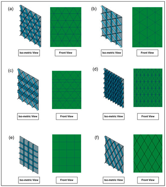
Figure 1.
Aerospace grid panels: (a) isometric, (b) isometric II, (c) anisogrid, (d) bi-grid, (e) waffle, (f) X-grid.

Table 1.
Material properties of aluminum alloy 7075-T6.
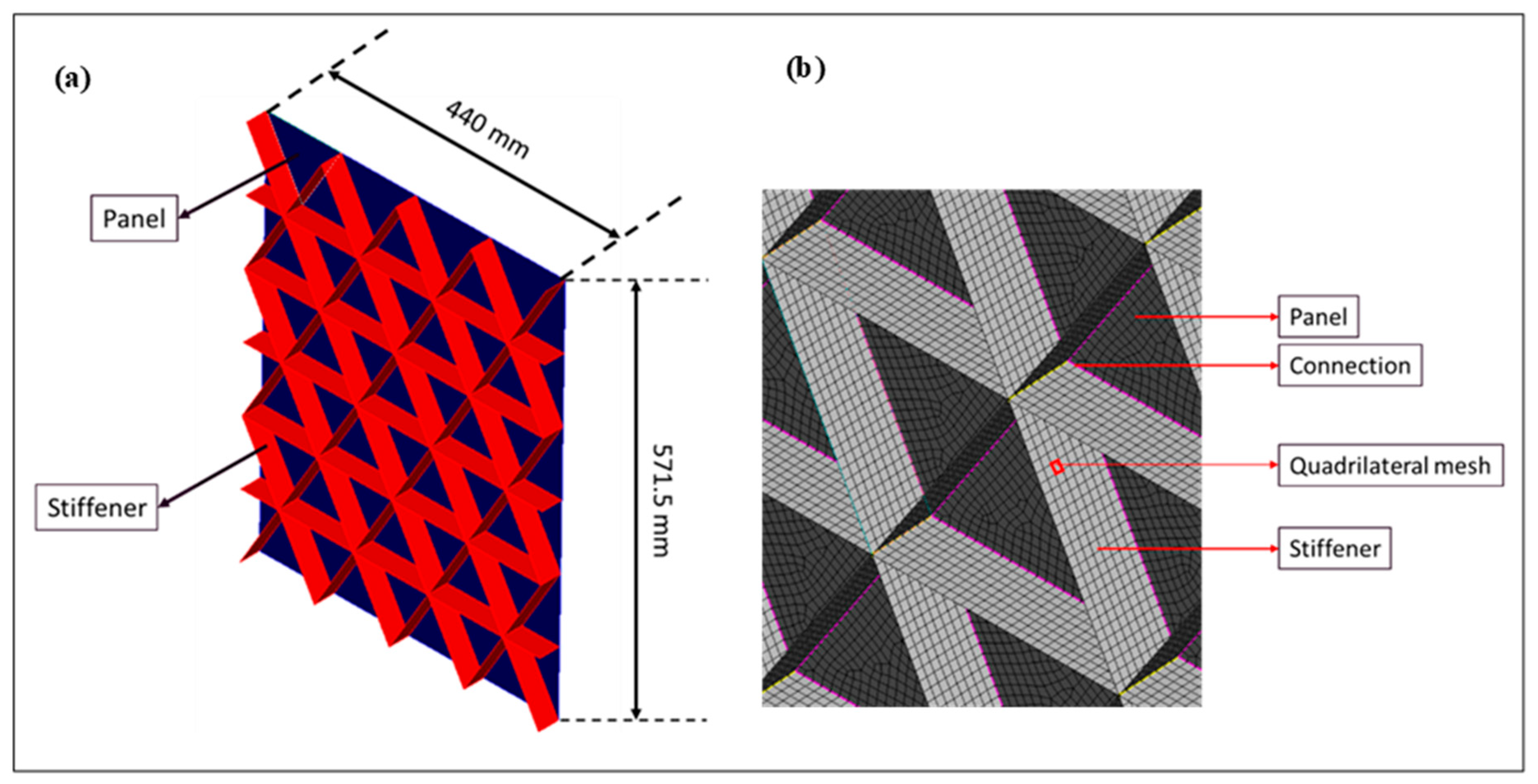
The six different stiffened panels were designed with ANSYS Design Modeler 2022 R1 (Ansys, Inc., Canonsburg, PA, USA), and the front view of the panels is illustrated in Figure 1. The height of the panel is kept as 571.5 mm, while the length is 440 mm. An isometric view of one of the panels is shown in Figure 2. It is important to note that the panels are designed as surface bodies, which is appropriate for analyzing thin-walled structures such as stiffened panels.

Figure 2.
(a) Isometric view of the panel; (b) mesh and body connection.
Quadrilateral elements are selected for the meshing of the panel. The connections between the panel and the stiffeners are evaluated to ensure proper bonding and to confirm that all components function together as a single unit during the simulation, as shown in Figure 2. The mesh size is set to 10 mm, validated against the same authors’ literature [41]. The boundary conditions are also consistent with the experimental setup of aircraft stiffened panels, where all edges are assumed to be supported for numerical solutions [41]. For the linear buckling analysis, a force of 1 kN is applied to both the upper and lower ends of the panel, along with the boundary conditions illustrated in Figure 3 [22].
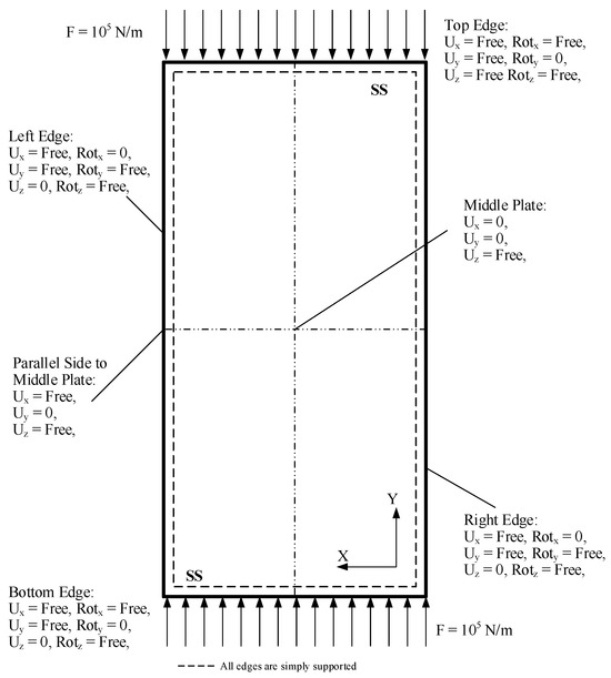
Figure 3.
Boundary conditions of the panel, reprinted from Ref. [22].
2.2. Artificial Neural Network
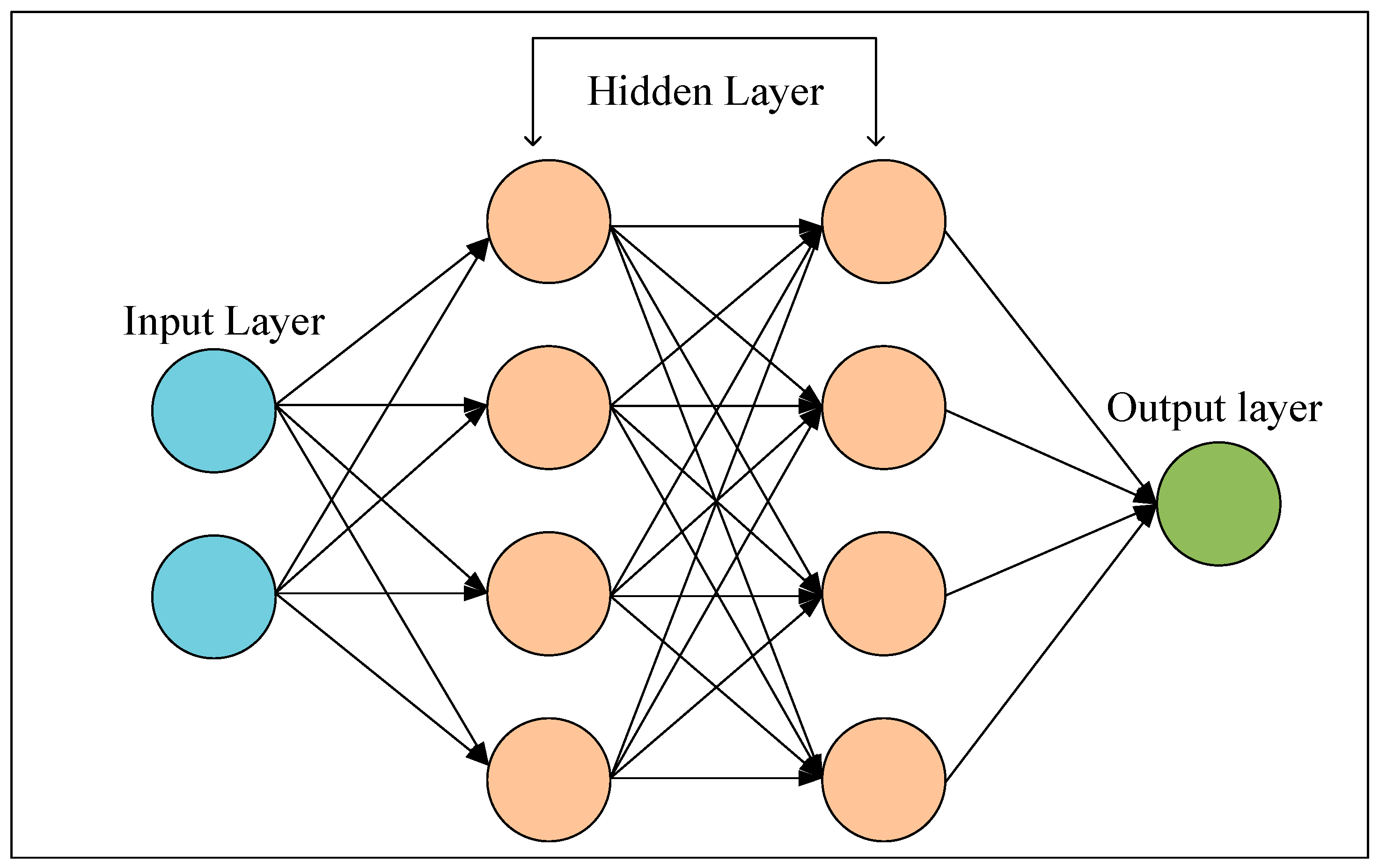
An artificial neural network (ANN) is a subset of machine learning (ML) that functions by mimicking the working mechanism of a brain [42]. An ANN consists of one input layer, one output layer, and multiple hidden layers—depending on the requirement. These layers are interconnected nodes, known as neurons, linked by weighted connections or synapses to recognize the data pattern, train or learn from it, and make decisions [43]. The input layer takes in data; the hidden layers (which can be multiple) utilize the input data and process them employing weights, biases, and activation functions; and the output layer predicts or classifies the results depending on the type of task. For their multilayered decision-making architecture, in most cases, an ANN outperforms classical models [44,45]. Figure 4 shows the general architecture of an ANN.

Figure 4.
ANN model architecture.
The weights (W) and biases (b) are very crucial for the learning process, as weight quantitatively represents the strength between neurons and also determines the influence of the input value on the output, and biases help shift the activation functions to improve the performance of the model [46]. In addition, the activation function introduces nonlinearity to the model for better learning capability [47]. Some activation functions are suitable for regression analysis, while others perform better for classification models. Table 2 summarizes different activation functions, working principles, and advantages.
Table 2.
Activation functions.
2.3. Decision Tree
A decision tree or DT algorithm is a robust algorithm in ML that utilizes a hierarchical tree structure for classifying or forecasting data [48,49]. The DT architecture is constructed by partitioning into nodes, branches, and leaves. Each node represents decision-based feature values, the branches of the tree connect different nodes and illustrate the decision rule, and tree leaves represent the outcome. One of the major advantages of this algorithm is the interpretability of the results, and therefore, the application of the DT algorithm is widespread [50]. However, the major drawback includes the susceptibility to overfitting [49].
2.4. KNN
The k-nearest neighbors (KNN) algorithm is a nonparametric ML algorithm widely used in ML applications. This classical model predicts a value based on their closest neighboring points from the trained dataset [34]. The nearest neighbors are chosen utilizing suitable distance metrics, i.e., Euclidian distance [34]. It uses a variable called ‘k’ that defines the number of ‘nearest neighbors’. Once k-nearest values are determined, it performs majority voting for the classification tasks [51]. For the regression tasks, an average value of the nearest data point determines the predicted outcome [52]. The optimum value of ‘k’ is determined by the hyperparameter tuning.
2.5. Random Forest Regression
Random forest is a broadly used ML algorithm method that employs ensemble techniques to perform numerous regression or classification tasks [53]. Random forest regression, as employed in this study, is quite popular as it reduces overfitting and improves generalization [54]. This algorithm randomly splits the dataset into multiple subsets through bootstrapping. During the splitting of the dataset, each decision tree is exposed to different points of the dataset, which improves the robustness of the model and reduces the variance. Each decision tree is trained independently to attain the prediction from each instance. Once trained, the output prediction from the individual tree is averaged to obtain the final prediction [55,56].
2.6. XGBoost
Extreme Gradient Boosting (XGBoost) is an ensemble learning method that employs gradient-boosted decision trees to forecast the target values. This highly scalable model exhibits superior performance with low computational complexity [57]. This enhances the performance of the GBDT algorithm [58]. GBDT is an iterative technique that constructs an ensemble of weak learners or trees sequentially, where each new tree corrects the errors of the prior iterations. It enhances the GBDT models by implementing advanced regularization methods (L1 or L2) to mitigate overfitting. The major advantage of regression analysis using XGBoost is that it deals with missing values [59].
2.7. CatBoost
The category boosting algorithm (CatBoost) utilizes an ensemble technique derived from the Gradient Boosting Decision Tree (GBDT) [60]. It is a robust technique used to handle noisy data with heterogeneous features [61]. Like the XGboost algorithm, Catboost utilizes the regularization method to overcome overfitting. One of the major advantages of this algorithm is that it does not require any preprocessing of categorical features. In addition, CatBoost also introduces a permutation-driven algorithm for ordered boosting [60]. For this reason, the Catboost algorithm outperforms other GBDTs for regression tasks [62,63].
2.8. LightGBM
LightGBM was first designed using the Gradient Boosting framework to achieve high efficiency, performance, and scalability [64]. To enhance accuracy and training speed, this algorithm utilizes a leaf-wise tree growth strategy [65], which differs from level-wise growth by selecting the leaf with the highest loss reduction for further splitting. In addition, LightGBM utilizes a histogram-based algorithm to effectively handle large datasets and reduce memory consumption by grouping continuous feature values into discrete bins [66]. Due to its speed, accuracy, and ability to process large-scale data, LightGBM is well-suited for regression tasks.
3. Data Acquisition and Preparation
3.1. Latin Hypercube Sampling
The aim of this research is to predict the critical buckling load (Pcr) while varying the thickness of the plate (Pt), the height of the stiffeners (Sh), the thickness of the stiffeners (St), and the mass of the plate (Mplate) utilizing ML and ANN algorithms. To generate design points for the study, the Latin Hypercube Sampling (LHS) method was employed in the Ansys parametric study platform.
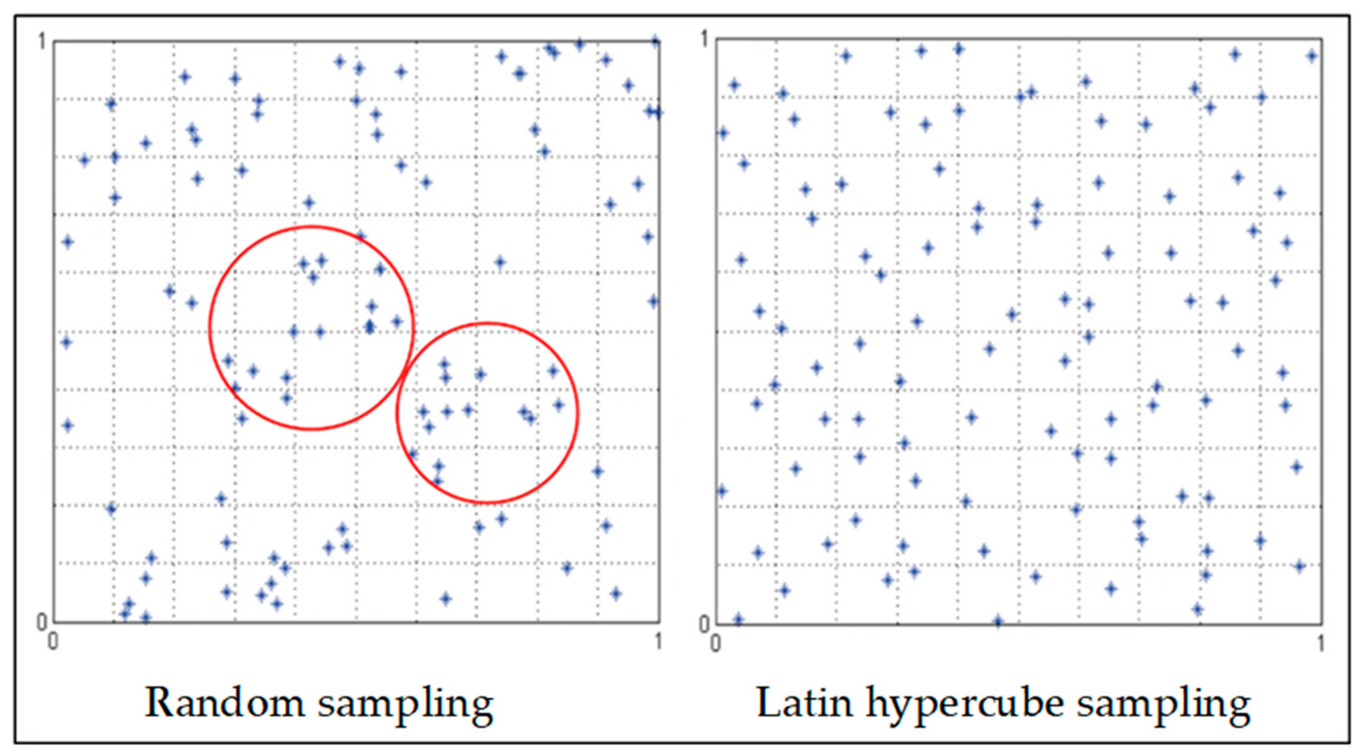
LHS is a stratified sampling method that divides each dimension of the dataset into equal intervals (or strata). Samples from each dimension are drawn randomly from each interval or stratum to ensure a uniform and non-overlapping distribution of data based on their corresponding probability density function [67]. The overall sampling is completed by randomly combing the dimension-specific samples to produce the design points [68]. Unlike random sampling, the LHS method ensures a reduced correlation between design points and the participation of each type of dataset [69], as shown in Figure 5.

Figure 5.
Comparison between random sampling and LHS (Reprinted from Ref. [69]).
For creating data points, each variable’s upper and lower bound was defined, as shown in Table 3. For each type of grid panel, a sample size of 1000 was selected, and in total, 6000 design points were generated. It is important to note that each input variable (Pt, Sh, St, and Mplate) was divided into strata. Then, 1000 design points (DPs) were randomly drawn from each stratum, ensuring a uniform distribution of samples.
Table 3.
Upper and lower bound of variables.
3.2. Data Processing
3.2.1. One Hot Encoding
After the results from the parametric study were acquired, all the categorical data, such as types of grid patterns, were transformed into binary representation using one hot encoding. Each grid type was assigned a unique binary feature, as shown in Table 4. For instance, the value of ‘1’ in the “Anisogrid” column indicates that the row corresponds to the “Anisogrid” panel; meanwhile, the values in columns representing other grids remain 0, as this row is not representative of their corresponding values. This transformation is required for the ML and ANN models to process the categorical data without assuming ordinal relationships between different grid types.
Table 4.
Representation of dataset using one hot encoding.
3.2.2. MinMax Scalar
MinMax Scalar is a prerequisite for data processing that transforms the dataset’s features (x) into a normalized value with a specific range (i.e., 0, 1). Normalization of the data is required when the scale of the feature values drastically differs [70]. MinMax Scalar transforms the data into a ratio, where the maximum value of the data will give an output of 1 and the minimum value will provide an output value of 0. This scaling or normalizing process is conducted using the following equation:
where
;
In this research, analysis was conducted both with and without normalizing the input features to understand the importance of data pre-processing. Table 5 presents one sample from each category after the normalization of the dataset.
Table 5.
Sample of scaled data (normalization).
3.2.3. Performance Evaluation Metrics
The following performance evaluation metrics were utilized for the evaluation of the ML and ANN models in this research. MSE, MAE, RMSE, and R2 were utilized for evaluating the initial performance of the model. Afterward, the standard deviation (STD) and coefficient of correlation (R) were used to check the testing and training performance. STD and R were utilized for plotting Taylor diagrams.
Here,
SSR = sum of squares regression;
SST = total sum of squares.
3.2.4. Hyperparameter Optimization for ML and ANN
First, the hyperparameters of classical ML algorithms with their ranges are shown in Table 6. For the case of ANN hyperparameter optimization, a trial-and-error method is adopted, and the different combinations of the hyperparameters are shown in Table 7.
Table 6.
Studied hyperparameters for ML models.
Table 7.
Studied hyperparameters for ANN models.
3.3. Overfitting Control and Generalization
Before model training began, the dataset was divided into 80% for training and 20% for testing to reduce the risk of overfitting and enhance generalization. The artificial neural network (ANN) model used early stopping and ReduceLROnPlateau callbacks. These features halted training when the validation loss stabilized and lowered the learning rate adaptively. Additionally, overfitting was assessed by comparing the model’s performance on the training and testing datasets using Taylor diagrams.
The ANN model used in this research was implemented with TensorFlow 2.11/Keras. In contrast, classical machine learning models were developed using Scikit-learn 1.2 in a Python 3.9 environment on the Jupyter Notebook 7.2.3 platform. The model was trained with the Nadam optimizer, using a learning rate of 0.0025 and a batch size of 8. Mean squared error (MSE) served as the loss function. Although a maximum of 300 epochs was set for training, the model typically converged between 80 and 120, thanks to the EarlyStopping and ReduceLROnPlateau callbacks. All training was conducted on a Windows 11 machine with a 12th Gen Intel Core i7 processor (Intel Corporation, Santa Clara, CA, USA) and 16 GB of RAM, without GPU support.
4. Performance Optimization of ANN Model
4.1. Activation Function
The activation function (AF) plays a vital role in refining prediction in neural networks. Different combinations of the AF have been tested to achieve optimized results. To ensure a fair comparison of the optimized results, the number of neurons (network architecture), optimizers, batch numbers, and initial learning rate are kept constant across all configurations while testing the AF.
From the analysis, as shown in Table 8, it is found that the best performing AF configuration is selu/relu/relu/relu/linear/linear/selu/1, with the lowest MSE value of 7.3698, MAE value of 1.7741, and RMSE value of 2.7147 and a high R2 score of 0.9996. Apart from that, the constant AF configuration of elu/elu/elu/elu/elu/elu/elu/1 also performed remarkably, achieving an MSE value of 12.0609, MAE value of 1.9229, and RMSE value of 3.4728, with a high R2 score of 0.9994. Similarly, the performance of selu/selu/selu/selu/selu/selu/selu/1 is slightly inferior to the elu/elu/elu/elu/elu/elu/elu/1 configuration, with an MSE value of 14.4777, an MAE value of 2.2816, an RMSE value of 3.8049, and a high R2 of 0.9992.
Table 8.
Selective configuration of AF with benchmarks.
For the ‘relu’-only AF, the performance degrades significantly, with 88.5 times higher MSE (652.46), 9.22 times higher MAE (16.3625), and 9.41 times higher RMSE (25.5434) than the best-performing configuration. The configuration of linear/linear/linear/linear/linear/linear/linear/1 performance was significantly poor. The configuration involving sigmoid and softmax shows poor performance, with negative R2 scores of 0.0025 and 0.0018.
4.2. Neuron Architecture
For the analysis of neuron architecture, the number of neurons is progressively reduced for each model, creating a funnel-like structure, as found in Table 9. This progressively reduced number of neurons is employed to avoid any unnecessary complexity in the networking system. For choosing the optimum composition of the dense layers or the architecture of the model, each configuration was trained using the same dataset, optimization algorithm, and hyperparameters to ensure a fair comparison. The last layer of the network was kept 1 for numerical value prediction.
Table 9.
Benchmark of the models based on neural architecture.
From the table, it is evident that, with the increase in the complexity of the model, the MSE, MAE, and RMSE values are reduced with an increased R2 score. Among all models, Model 1 (200/100/50/25/12/6/3/1) outperforms the others, attaining the lowest value of MSE at 7.3698, MAE at 1.7741, and RMSE at 2.7147, with the highest R2 value among other models. Model 2 (128/64/32/16/8/4/2/1) performs reasonably well with an MSE value of 11.59, an MAE value of 2.1179, an RMSE value of 3.4055, and an R2 score of 0.9994. From Model 3 to Model 6, the performance reduction is noticeable with the reduction in the network’s complexity. This performance reduction may indicate that there may not be enough neurons to learn the underlying complexity of the data.
4.3. Batch Size, Optimizers, and Learning Rates
This section presents an intensive analysis conducted to find the optimum batch sizes, suitable optimizers, and initial learning rates. As optimizers like Adagrad and Adadelta did not perform well, only results obtained from Nadam, Adam, and RMSprop optimizers are included in Table 10, Table 11, Table 12 and Table 13. Two sets of experiments were carried out using the previously mentioned parameters. One was without scaling data, and the other was with the normalization of data with MinMax Scalar.
Table 10.
Performance comparison table for batch 4, with and without scaling of data.
Table 11.
Performance comparison table for batch 8, with and without scaling of data.
Table 12.
Performance comparison table for batch 12, with and without scaling of data.
Table 13.
Performance comparison table for batch 16, with and without scaling of data.
4.3.1. Batch Size 4
From Table 10, it is observed that the best-performing optimizer for this dataset is Nadam with an initial learning rate (LR) of 0.001, which provides an MSE value of 3.1768, MAE value of 0.9563, and RMSE value of 1.7823. This value is observed when the input data is scaled with MinMax Scalar. The second-best optimizer for our prediction is RMSprop (LR = 0.0025), which has a 5.8% increased MSE value (3.3712) and a 17.1% increased MAE value (1.1537). Similarly, without scaling, however, Nadam optimizers significantly outperform other optimizers. It is important to note that the R2 score is almost identical for all the models.
4.3.2. Batch Size 8
Next, from Table 11, it is found that with batch size 8, the Nadam optimizer with LR = 0.0025 achieves the best benchmark with or without scaling of the dataset. With scaling, the Nadam optimizer (LR = 0.0025) records the lowest MSE (2.9584), MAE (0.9875), and RMSE (1.72) values of all the models across all batch sizes. Similarly, without scaling, it outperforms every other result across any configuration, making it the optimum parameter for our dataset.
4.3.3. Batch Size 12
As shown in Table 12, the Nadam optimizer significantly outperforms other optimizers without scaling. The lowest MSE value obtained by the Nadam optimizer (LR = 0.0025) is 5.0690, and with scaling, the best results are obtained with the Nadam optimizer (LR = 0.005).
4.3.4. Batch Size 16
As calculated in Table 13, Nadam outperforms all models with batch size 16, as in previous cases. The best-performing configuration is Nadam, with LR = 0.0025. With scaling, it achieves an MSE score of 3.0523, and without scaling, the Nadam optimizer (LR = 0.005) achieves an MSE score of 5.2145. This indicates the importance of choosing the appropriate optimizers and scaling datasets in the ANN models.
In a nutshell, feature scaling has significantly affected the model’s performance. For Nadam (LR = 0.0025), the feature scaling improves MSE values by up to 53% and MAE values by up to 32.5%. Other optimizers, like RMSprop and Adam, also perform significantly better with MinMax Scalar. In addition, the Nadam optimizer performed better, with a learning rate of 0.001 to 0.0025. RMSprop, however, performed consistently with an LR of 0.001.
The effectiveness of Nadam (Nesterov-accelerated Adaptive Moment) stems from its integration of the adaptive learning rates characteristic of Adam and the Nesterov momentum update. This combination enables Nadam to harness the robustness of Adam’s adaptive learning while also benefiting from the predictive capabilities of Nesterov momentum, which anticipates future gradients. As a result, Nadam can achieve faster convergence and better generalization in complex tasks, such as buckling prediction [71].
5. Comparing ANN and ML Models
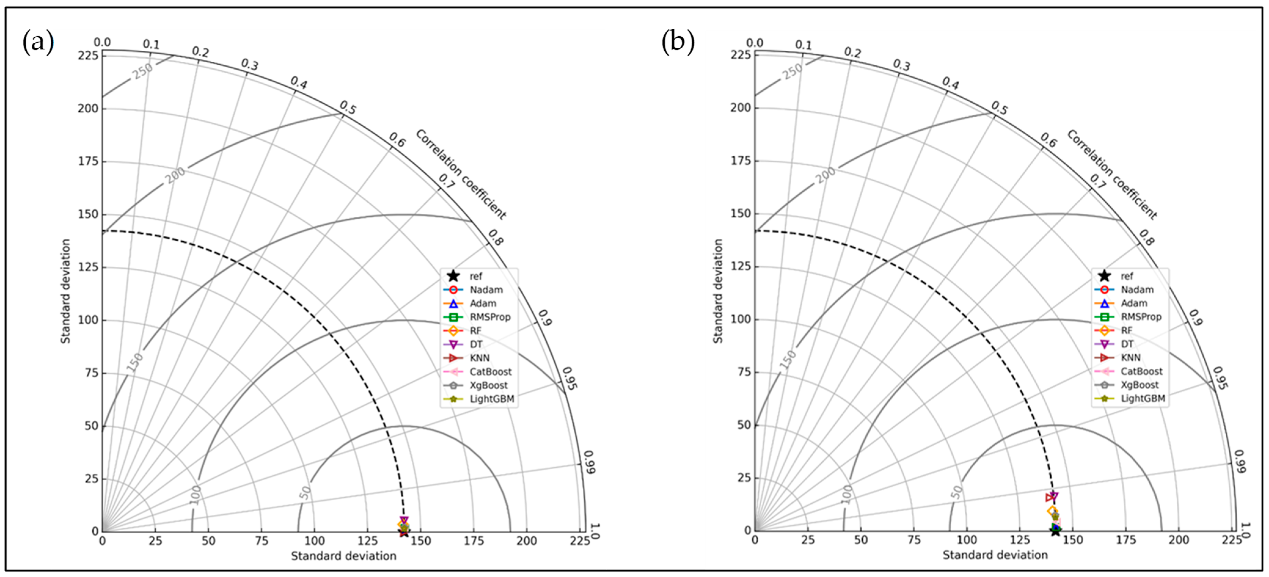
First, this section compares the best-performing ANN models with classical ML models based on their performance during training and testing using a Taylor diagram, as shown in Figure 6. Next, the test data performance is evaluated using the evaluation metrics explained earlier. ANN models with three different optimizers and the best RMSE values were chosen for the evaluation process. The Taylor diagram was constructed utilizing the training and testing datasets’ standard deviation (STD) and correlation coefficient (R). The diagram illustrates the relationship between the predicted values relative to the actual data.
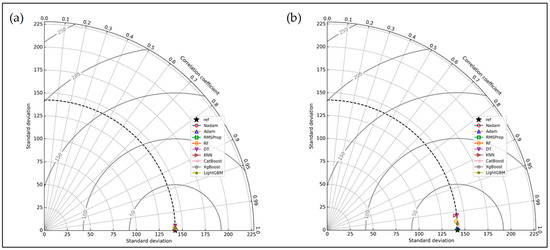
Figure 6.
(a) Taylor diagram of training datasets of different models; (b) Taylor diagram of testing datasets of different models.
Figure 6a illustrates that the training data for all the models almost cluster around the actual data, indicating the model is well-trained for the prediction.
In the testing dataset, from Figure 6b, it is noticed that the decision tree and k-nearest-neighbors algorithm results are distant from the actual value. The Train r = 1.0 for KNN and Test r = 0.9936 indicate a possible overfitting during the training session.
The ANN models (all three of them) performed better, indicating that they have generalized well to unseen data and are not overfitting during the training. The boosting algorithms also generalized well, and their R values did not deviate from the trained dataset.
The prediction performance of different models was evaluated based on the performance metrics mentioned previously. The results, presented in Table 14, show that the ANN models (all three of them) significantly outperform traditional ML models. As mentioned in the previous section, ANN with Nadam performs best among all the ANN models, and it outperforms other traditional ML models with a 2.9584 MSE score.
Table 14.
Performance evaluation.
On the other hand, classical models such as RF and DT show significantly high errors. Among all the models, DT has the highest MSE (270.1035) and RMSE (16.4348), showing poor generalization and high variance. Similarly, the RF model exhibits poor performance with high error values (MSE = 93.2298 and RMSE = 9.6556).
The KNN model also performs poorly, with a high MSE value of 127.8302 and RMSE of 11.3062. This poor performance might occur due to overfitting of the training dataset, as the training coefficient of correlation value for the KNN model was 1.00.
The CatBoost algorithm performed the best among all the ML models, with an MSE value of 17.6968 and an RMSE value of 4.2067. Other boosting methods, such as LightGBM and XGBoost, performed better than other ML models. LightGBM had an MSE value of 42.1116 and an RMSE value of 6.4893; on the other hand, XGBoost had an MSE value of 53.9406 and an RMSE of 7.3444.
In summary, the artificial neural network models consistently outperformed the traditional machine learning models mentioned in this article. Even the worst-performing ANN models outperformed the ML models in many cases, demonstrating the superior predictive robustness and accuracy of ANN models.
Feature Importance Analysis
Figure 7 illustrates a detailed SHAP-based analysis of the importance of features in predicting critical buckling load for various stiffened panel configurations studied in the present study.
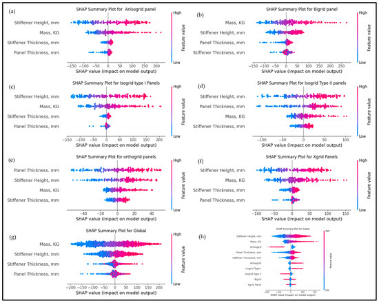
Figure 7.
SHAP (SHapley Additive exPlanations) summary plots: (a) anisogrid panel, (b) bi-grid panel, (c) isogrid type I panel, (d) isogrid type I panel, (e) orthogrid panel, (f) X-grid panel, (g) global analysis combining all panel types, and (h) mean absolute SHAP values for all features and panel types.
Figure 7a–f represent SHAP summary plots for individual panel types—anisogrid, bigrid, isogrid type I, isogrid type II, orthogrid, and X-grid—illustrating how feature contributions differ based on geometry. Stiffener height and mass are consistently suggested as the most influential features in most panel types, positively affecting buckling strength. Panel thickness is particularly significant for orthogrid panels (e), while stiffener thickness also plays a substantial role across all kinds. As shown in Figure 7g, the global analysis aggregates data from all configurations, reaffirming the importance of mass, stiffener height, and stiffener thickness. Finally, Figure 7h summarizes the mean absolute SHAP values across all panels, confirming that stiffener height and mass are critical factors regardless of panel type.
These findings highlight the importance of careful selection and adjusting geometric parameters—especially stiffener dimensions—to enhance structural stability. Material properties like Young’s modulus and density were excluded from this analysis, as they were constant in the current study.
6. Limitations and Future Scope
Despite the promising outcomes of this study, several limitations should be acknowledged for future research directions.
6.1. Direction 1: Advanced Models
This study is limited to traditional ML models and Multilayer Perceptron (MLP)-based ANN architectures. However, it excluded more advanced deep learning models such as convolutional neural networks (CNNs), recurrent neural networks (RNNs), or ensemble architectures.
6.2. Direction 2: Expanding Data Size
A total of 6000 design points (1000 for each grid panel) were generated utilizing the Latin Hypercube Sampling (LHS) technique in the Ansys parametric study platform. In general, 6000 design points are enough for structural analysis; potential overfitting risk remains a concern for this study. Future research should consider expanding the dataset through additional simulation or by experimental means to enhance the robustness of the study.
6.3. Direction 3: Complex Neural Network Architecture
Although ANN and traditional ML regression models were employed, the study solely depended on the MLP architecture with a funnel-like structure. While this configuration is effective and reduces the complexity of the model, it might not fully capture the complex features that could be introduced with the increasing number of patterns.
6.4. Direction 4: Generalization and Transfer Learning
While the ANN model demonstrated excellent predictive accuracy within this dataset, its generalization to unseen geometries or alternative materials—such as composite laminates or titanium alloys—was not investigated. These material systems may exhibit distinct mechanical behavior, failure mechanisms, and buckling responses that differ from the patterns learned by the current model. To address this, future research could explore integrating transfer learning techniques, allowing the pre-trained ANN model to be retrained or fine-tuned using a smaller dataset of new materials or geometric configurations.
7. Conclusions
This study employed different ML algorithms and ANN models to predict the buckling load of six metallic grid-structured panels. The primary objective of this research was to develop a robust ML model that can accurately predict buckling loads under different geometric conditions. A strong 6000 data points were created, and the simulation outcomes were tested utilizing various ML models such as RF, XGboost, LightGBM, CatBoost, DT, and ANN models. The results were predicted with and without the normalization of the data. The results were evaluated using MAE, MSE, RMSE, and R2 scores.
The findings show the following:
- ANN models performed better with a 200/100/50/25/12/6/3/1 neural configuration. For this study, the best activation configuration is selu/relu/relu/relu/linear/linear/selu/1.
- ANN models with the Nadam optimizer performed significantly better than others in this study.
- Normalization or feature scaling significantly improves the model’s prediction, which this study endorses. Normalization improves MSE values by up to 53% and MAE values by up to 32.5%.
- The Nadam optimizer, with a learning rate of 0.0025 and batch size of 8, outperformed all other ANN configurations and ML algorithms. The best model configuration achieves an MSE value of 2.9584, an MAE value of 0.9875, an RMSE value of 1.72, and an R2 score of 0.9998. It significantly outperforms other models.
- This proposed ANN model significantly outperforms other classical algorithms. Compared to the best-performing classical model (CatBoost), our proposed ANN model has an almost 6-fold better MSE value, a 2.68-fold better MAE value, a 2.5-fold better RMSE value, and a nearly identical R2 score.
- Taylor’s diagram highlights that all ANN models (three different optimizers with the best results) had better training and testing performance, indicating these ANN models have generalized well to the unseen data and have not been overfitted.
- SHAP analysis reveals that stiffener height and mass are the most influential features affecting critical buckling load, highlighting the importance of geometric optimization for enhancing panel stability.
After an extensive study, it is safe to conclude that the ANN model outperforms the classical ML models in predicting the linear buckling load of metallic grid-structured panels. Other neural network models, such as recurrent neural networks and convolutional neural networks, have not been studied in this study and will be studied in future work.
Author Contributions
Conceptualization, S.K. and S.B.R.; Methodology, S.K. and S.B.R.; Software, S.K. and S.B.R.; Formal Analysis, S.K., M.M.R., and J.S.; Investigation, S.B.R., M.M.R., and J.S.; Resources, M.M.R., J.S., and G.V.; Data Curation, J.S. and G.V.; Writing—Original Draft Preparation, S.K. and S.B.R.; Writing—Review and Editing, M.M.R., J.S., and G.V.; Visualization, S.K. and M.M.R.; Supervision, S.B.R. and G.V.; Project Administration, S.B.R. and G.V. All authors have read and agreed to the published version of the manuscript.
Funding
This research received no external funding.
Data Availability Statement
The datasets presented in this article are not readily available because they are part of an ongoing study and are currently under further analysis. Requests to access the datasets should be directed to the corresponding author.
Acknowledgments
The authors acknowledge the use of Grammarly, an AI-based language editing tool, to assist in improving the clarity and grammatical correctness of the manuscript. No content was generated by Grammarly; its use was limited to language refinement under the authors’ full supervision.
Conflicts of Interest
The authors declare no conflicts of interest.
References
- Jones, R.M. Buckling of Bars, Plates, and Shells; Bull Ridge: Blacksburg, VA, USA, 2006. [Google Scholar]
- Hilburger, M.W. The Development of Shell Buckling Design Criteria Based on Initial Imperfection Signatures; World Scientific Connect: Singapore, 2008. [Google Scholar]
- Abramovich, H. Experimental Studies of Stiffened Composite Panels Under Axial Compression, Torsion and Combined Loading; World Scientific Connect: Singapore, 2008. [Google Scholar]
- Bisagni, C. Buckling and Postbuckling Tests on Stiffened Composite Panels and Shells; World Scientific Connect: Singapore, 2008. [Google Scholar]
- Kling, A. Stability Design of Stiffened Composite Panels—Simulation and Experimental Validation; World Scientific Connect: Singapore, 2008. [Google Scholar]
- Yamada, S.; Uchiyama, M. Imperfection-Sensitive Buckling and Postbuckling of Spherical Shell Caps; World Scientific Connect: Singapore, 2008. [Google Scholar]
- Aliabadi, M.H.; Baiz, P.M. The Boundary Element Method for Buckling and Postbuckling Analysis of Plates and Shells; World Scientific Connect: Singapore, 2008. [Google Scholar]
- Wadee, M.A. Nonlinear Buckling in Sandwich Struts: Mode Interaction and Localization; World Scientific Connect: Singapore, 2008. [Google Scholar]
- Błachut, J. The Use of Composites in Underwater Pressure: Hull Components; World Scientific Connect: Singapore, 2008. [Google Scholar]
- Riccio, A.; Garofano, A.; Rigliaco, G.; Boccaccio, M.; Acerra, F. Redesign of an Aeronautical Composite Stiffened Panel with the Double-Double Design Approach. In Proceedings of the 34th Congress of the International Council of the Aeronautical Sciences, Florence, Italy, 9–13 September 2024; pp. 1–14. [Google Scholar]
- Murphy, A.; Price, M.; Lynch, C.; Gibson, A. The Computational Post-Buckling Analysis of Fuselage Stiffened Panels Loaded in Shear. Thin-Walled Struct. 2005, 43, 1455–1474. [Google Scholar] [CrossRef]
- Chandra, D.; Nukman, Y.; Azka, M.A.; Sapuan, S.M.; Yusuf, J. Review on Integral Stiffened Panel of Aircraft Fuselage Structure. Def. Technol. 2024, 46, 1–11. [Google Scholar] [CrossRef]
- Elumalai, E.S.; Asokan, R.; Thejus, C.M.; Uday Ranjan Goud, N.; Sivamani, S. Numerical Investigations of the Buckling Behaviour of an Integrated Stiffened Panel. J. Phys. Conf. Ser. 2024, 2837, 012063. [Google Scholar] [CrossRef]
- Zhang, G.; Hu, Y.; Yan, B.; Tong, M.; Wang, F. Buckling and Post-Buckling Analysis of Composite Stiffened Panels: A Ten-Year Review (2014–2023). Thin-Walled Struct. 2024, 205, 112525. [Google Scholar] [CrossRef]
- Huang, Y.; Zhang, Y.; Kong, B.; Gu, J.; Wang, Z.; Chen, P. Experimental and Numerical Studies on Buckling and Post-Buckling Behavior of T-Stiffened Variable Stiffness Panels. Chin. J. Aeronaut. 2024, 37, 459–470. [Google Scholar] [CrossRef]
- Linde, P.; Pleitner, J.; Rust, W. Virtual Testing of Aircraft Fuselage Stiffened Panels. In Proceedings of the 24th Congress of the International Council of the Aeronautical Sciences, Yokohama, Japan, 29 August–3 September 2004; pp. 1–9. [Google Scholar]
- Wang, Y.; Wang, F.; Jia, S.; Yue, Z. Experimental and Numerical Studies on the Stability Behavior of Composite Panels Stiffened by Tilting Hat-Stringers. Compos. Struct. 2017, 174, 187–195. [Google Scholar] [CrossRef]
- Degenhardt, R.; Kling, A.; Rohwer, K.; Orifici, A.C.; Thomson, R.S. Design and Analysis of Stiffened Composite Panels Including Post-Buckling and Collapse. Comput. Struct. 2008, 86, 919–929. [Google Scholar] [CrossRef]
- Jin, B.C.; Li, X.; Mier, R.; Pun, A.; Joshi, S.; Nutt, S. Parametric Modeling, Higher Order FEA and Experimental Investigation of Hat-Stiffened Composite Panels. Compos. Struct. 2015, 128, 207–220. [Google Scholar] [CrossRef]
- Elumalai, E.S.; Krishnaveni, G.; Sarath Kumar, R.; Dominic Xavier, D.; Kavitha, G.; Seralathan, S.; Hariram, V.; Micha Premkumar, T. Buckling Analysis of Stiffened Composite Curved Panels. Mater. Today Proc. 2020, 33, 3604–3611. [Google Scholar] [CrossRef]
- Bouazizi, M.; Lazghab, T.; Soula, M. Mechanical Response of a Panel Section with a Hexagonally Tessellated Stiffener Grid. Proc. Inst. Mech. Eng. Part G J. Aerosp. Eng. 2017, 231, 1402–1414. [Google Scholar] [CrossRef]
- Sarwoko, A.R.K.; Prabowo, A.R.; Ghanbari-Ghazijahani, T.; Do, Q.T.; Ridwan, R.; Hanif, M.I. Buckling of Thin-Walled Stiffened Panels in Transportation Structures: Benchmarking and Parametric Study. Eng. Sci. 2024, 30, 1137. [Google Scholar] [CrossRef]
- Mojtabaei, S.M.; Becque, J.; Hajirasouliha, I.; Khandan, R. Predicting the Buckling Behaviour of Thin-Walled Structural Elements Using Machine Learning Methods. Thin-Walled Struct. 2023, 184, 110518. [Google Scholar] [CrossRef]
- Kaveh, A.; Dadras Eslamlou, A.; Javadi, S.M.; Geran Malek, N. Machine Learning Regression Approaches for Predicting the Ultimate Buckling Load of Variable-Stiffness Composite Cylinders. Acta Mech. 2021, 232, 921–931. [Google Scholar] [CrossRef]
- Gupta, M.; Prakash, S.; Ghani, S.; Paramasivam, P.; Ayanie, A.G. Integrating PCA and XGBoost for Predicting UACLC of Steel-Reinforced Concrete-Filled Square Steel Tubular Columns at Elevated Temperatures. Case Stud. Constr. Mater. 2025, 22, e04456. [Google Scholar] [CrossRef]
- Bai, X.; Yang, J.; Yan, W.; Qun, H.; Belouettar, S.; Hu, H. A Data-Driven Approach for Instability Analysis of Thin Composite Structures. Comput. Struct. 2022, 273, 106898. [Google Scholar] [CrossRef]
- Ly, H.B.; Le, T.T.; Le, L.M.; Tran, V.Q.; Le, V.M.; Vu, H.L.T.; Nguyen, Q.H.; Pham, B.T. Development of Hybrid Machine Learning Models for Predicting the Critical Buckling Load of I-Shaped Cellular Beams. Appl. Sci. 2019, 9, 5458. [Google Scholar] [CrossRef]
- Degtyarev, V.V.; Tsavdaridis, K.D. Buckling and Ultimate Load Prediction Models for Perforated Steel Beams Using Machine Learning Algorithms. J. Build. Eng. 2022, 51, 104316. [Google Scholar] [CrossRef]
- Mishra, B.B.; Kumar, A.; Samui, P.; Roshni, T. Buckling of Laminated Composite Skew Plate Using FEM and Machine Learning Methods. Eng. Comput. 2021, 38, 501–528. [Google Scholar] [CrossRef]
- Tariq, A.; Uzun, B.; Deliktaş, B.; Yayli, M.Ö. A Machine Learning Approach for Buckling Analysis of a Bi-Directional FG Microbeam. Microsyst. Technol. 2024, 31, 177–198. [Google Scholar] [CrossRef]
- Lee, H.G.; Sohn, J.M. A Comparative Analysis of Buckling Pressure Prediction in Composite Cylindrical Shells Under External Loads Using Machine Learning. J. Mar. Sci. Eng. 2024, 12, 2301. [Google Scholar] [CrossRef]
- Kaveh, A.; Eskandari, A.; Movasat, M. Buckling Resistance Prediction of High-Strength Steel Columns Using Metaheuristic-Trained Artificial Neural Networks. Structures 2023, 56, 104853. [Google Scholar] [CrossRef]
- Tahir, Z.u.R.; Mandal, P.; Adil, M.T.; Naz, F. Application of Artificial Neural Network to Predict Buckling Load of Thin Cylindrical Shells under Axial Compression. Eng. Struct. 2021, 248, 113221. [Google Scholar] [CrossRef]
- Rayhan, S.B.; Rahman, M.M.; Sultana, J.; Szávai, S.; Varga, G. Finite Element and Machine Learning-Based Prediction of Buckling Strength in Additively Manufactured Lattice Stiffened Panels. Metals 2025, 15, 81. [Google Scholar] [CrossRef]
- Reda, R.; Ahmed, Y.; Magdy, I.; Nabil, H.; Khamis, M.; Lila, M.A.; Refaey, A.; Eldabaa, N.; Elmagd, M.A.; Ragab, A.E.; et al. Wall Panel Structure Design Optimization of a Hexagonal Satellite. Heliyon 2024, 10, e24159. [Google Scholar] [CrossRef]
- Alhajahmad, A.; Mittelstedt, C. A Novel Grid-Stiffening Concept for Locally Reinforcing Window Openings of Composite Fuselage Panels Using Streamline Stiffeners. Thin-Walled Struct. 2022, 179, 109731. [Google Scholar] [CrossRef]
- Zhang, B.; Jin, F.; Zhao, Z.; Zhou, Z.; Xu, Y.; Chen, H.; Fan, H. Hierarchical Anisogrid Stiffened Composite Panel Subjected to Blast Loading: Equivalent Theory. Compos. Struct. 2018, 187, 259–268. [Google Scholar] [CrossRef]
- Kim, T.D. Fabrication and Testing of Thin Composite Isogrid Stiffened Panel. Compos. Struct. 2000, 49, 21–25. [Google Scholar] [CrossRef]
- Xu, Y.; Chen, H.; Wang, X. Buckling Analysis and Configuration Optimum Design of Grid-Stiffened Composite Panels. AIAA J. 2020, 58, 3653–3664. [Google Scholar] [CrossRef]
- Reda, R.; Ahmed, Y.; Magdy, I.; Nabil, H.; Khamis, M.; Refaey, A.; Eldabaa, N.; Elmagd, M.A.; Lila, M.A.; Ergawy, H.; et al. Basic Principles and Mechanical Considerations of Satellites: A Short Review. Trans. Aerosp. Res. 2023, 2023, 40–54. [Google Scholar] [CrossRef]
- Sultana, J.; Varga, G. Finite Element Analysis of Post-Buckling Failure in Stiffened Panels: A Comparative Approach. Machines 2025, 13, 373. [Google Scholar] [CrossRef]
- Sinkhonde, D.; Mashava, D. An Artificial Neural Network Approach to Predict Particle Shape Characteristics of Clay Brick Powder under Various Milling Conditions. Results Mater. 2025, 25, 100650. [Google Scholar] [CrossRef]
- Tareq, W.Z.T. (Artificial) Neural Networks. In Decision-Making Models; Academic Press: Cambridge, MA, USA, 2024; ISBN 9780443161476. [Google Scholar]
- Liu, J.; Huang, Q.; Ulishney, C.; Dumitrescu, C.E. Comparison of Random Forest and Neural Network in Modeling the Performance and Emissions of a Natural Gas Spark Ignition Engine. J. Energy Resour. Technol. 2022, 144, 032310. [Google Scholar] [CrossRef]
- Peace, I.C.; Uzoma, A.O.; Ita, S.A.; Iibi, S. A Comparative Analysis of K-NN and ANN Techniques in Machine Learning. Int. J. Eng. Res. 2015, V4, 420–425. [Google Scholar] [CrossRef]
- Nokeri, T.C. Solving Economic Problems Applying Artificial Neural Networks. In Econometrics and Data Science; Apress: Berkeley, CA, USA, 2022; pp. 161–188. [Google Scholar] [CrossRef]
- Sharma, S.; Sharma, S.; Anidhya, A. Understanding Activation Functions in Neural Networks. Int. J. Eng. Appl. Sci. Technol. 2020, 4, 310–316. [Google Scholar]
- Pathak, S.; Mishra, I.; Swetapadma, A. An Assessment of Decision Tree Based Classification and Regression Algorithms. In Proceedings of the 2018 3rd International Conference on Inventive Computation Technologies (ICICT), Coimbatore, India, 15–16 November 2018; pp. 92–95. [Google Scholar] [CrossRef]
- Koya, B.P.; Aneja, S.; Gupta, R.; Valeo, C. Comparative Analysis of Different Machine Learning Algorithms to Predict Mechanical Properties of Concrete. Mech. Adv. Mater. Struct. 2022, 29, 4032–4043. [Google Scholar] [CrossRef]
- Dabiri, H.; Farhangi, V.; Moradi, M.J.; Zadehmohamad, M.; Karakouzian, M. Applications of Decision Tree and Random Forest as Tree-Based Machine Learning Techniques for Analyzing the Ultimate Strain of Spliced and Non-Spliced Reinforcement Bars. Appl. Sci. 2022, 12, 4851. [Google Scholar] [CrossRef]
- Uddin, S.; Haque, I.; Lu, H.; Moni, M.A.; Gide, E. Comparative Performance Analysis of K-Nearest Neighbour (KNN) Algorithm and Its Different Variants for Disease Prediction. Sci. Rep. 2022, 12, 6256. [Google Scholar] [CrossRef]
- Sitienei, M.; Otieno, A.; Anapapa, A. An Application of K-Nearest-Neighbor Regression in Maize Yield Prediction. Asian J. Probab. Stat. 2023, 24, 1–10. [Google Scholar] [CrossRef]
- Zhang, H.; Zhou, A.; Zhang, H. An Evolutionary Forest for Regression. IEEE Trans. Evol. Comput. 2022, 26, 735–749. [Google Scholar] [CrossRef]
- Dodda, R.; Raghavendra, C.; Aashritha, M.; MacHerla, H.V.; Kuntla, A.R. A Comparative Study of Machine Learning Algorithms for Predicting Customer Churn: Analyzing Sequential, Random Forest, and Decision Tree Classifier Models. In Proceedings of the 2024 5th International Conference on Electronics and Sustainable Communication Systems (ICESC), Coimbatore, India, 7–9 August 2024; pp. 1552–1559. [Google Scholar] [CrossRef]
- Clark, J.S. Model Assessment and Selection. In The Elements of Statistical Learning; Springer: New York, NY, USA, 2020; ISBN 9780387848570. [Google Scholar]
- Kwak, S.; Kim, J.; Ding, H.; Xu, X.; Chen, R.; Guo, J.; Fu, H. Machine Learning Prediction of the Mechanical Properties of γ-TiAl Alloys Produced Using Random Forest Regression Model. J. Mater. Res. Technol. 2022, 18, 520–530. [Google Scholar] [CrossRef]
- Chen, T.; Guestrin, C. XGBoost: A Scalable Tree Boosting System. In Proceedings of the KDD ‘16: Proceedings of the 22nd ACM SIGKDD International Conference on Knowledge Discovery and Data Mining, New York, NY, USA, 13–17 August 2016; pp. 785–794. [Google Scholar] [CrossRef]
- Akbari, P.; Zamani, M.; Mostafaei, A. Machine Learning Prediction of Mechanical Properties in Metal Additive Manufacturing. Addit. Manuf. 2024, 91, 104320. [Google Scholar] [CrossRef]
- Dong, J.; Chen, Y.; Yao, B.; Zhang, X.; Zeng, N. A Neural Network Boosting Regression Model Based on XGBoost[Formula Presented]. Appl. Soft Comput. 2022, 125, 109067. [Google Scholar] [CrossRef]
- Wang, Q.; Yan, C.; Zhang, Y.; Xu, Y.; Wang, X.; Cui, P. Numerical Simulation and Bayesian Optimization CatBoost Prediction Method for Characteristic Parameters of Veneer Roller Pressing and Defibering. Forests 2024, 15, 2173. [Google Scholar] [CrossRef]
- Prokhorenkova, L.; Gusev, G.; Vorobev, A.; Dorogush, A.V.; Gulin, A. Catboost: Unbiased Boosting with Categorical Features. In Proceedings of the 32nd Conference on Neural Information Processing Systems (NeurIPS 2018), Montréal, QC, Canada, 2–8 December 2018; pp. 6638–6648. [Google Scholar]
- Paul, S.; Das, P.; Kashem, A.; Islam, N. Sustainable of Rice Husk Ash Concrete Compressive Strength Prediction Utilizing Artificial Intelligence Techniques. Asian J. Civ. Eng. 2024, 25, 1349–1364. [Google Scholar] [CrossRef]
- Jabeur, S.B.; Gharib, C.; Mefteh-Wali, S.; Arfi, W. Ben CatBoost Model and Artificial Intelligence Techniques for Corporate Failure Prediction. Technol. Forecast. Soc. Chang. 2021, 166, 120658. [Google Scholar] [CrossRef]
- Ke, G.; Meng, Q.; Finley, T.; Wang, T.; Chen, W.; Ma, W.; Ye, Q.; Liu, T.Y. LightGBM: A Highly Efficient Gradient Boosting Decision Tree. In Proceedings of the NIPS’17: Proceedings of the 31st International Conference on Neural Information Processing Systems, Long Beach, CA, USA, 4–9 December 2017; pp. 3147–3155. [Google Scholar]
- Shi, H. Best-First Decision Tree Learning. Master’s Thesis, University of Waikato, Hamilton, New Zealand, 1994. [Google Scholar]
- Wang, D.n.; Li, L.; Zhao, D. Corporate Finance Risk Prediction Based on LightGBM. Inf. Sci. 2022, 602, 259–268. [Google Scholar] [CrossRef]
- Li, C.-Q.; Yang, W. Essential Reliability Methods; Time-Depen.; Elsevier: Amsterdam, The Netherlands, 2023. [Google Scholar]
- Song, C.; Kawai, R. Monte Carlo and Variance Reduction Methods for Structural Reliability Analysis: A Comprehensive Review. Probabilistic Eng. Mech. 2023, 73, 103479. [Google Scholar] [CrossRef]
- Wang, Z.; Zhao, D.; Heidari, A.A.; Chen, Y.; Chen, H.; Liang, G. Improved Latin Hypercube Sampling Initialization-Based Whale Optimization Algorithm for COVID-19 X-Ray Multi-Threshold Image Segmentation. Sci. Rep. 2024, 14, 13239. [Google Scholar] [CrossRef]
- Kim, Y.-S.; Kim, M.K.; Fu, N.; Liu, J.; Wang, J.; Srebric, J. Investigating the Impact of Data Normalization Methods on Predicting Electricity Consumption in a Building Using Different Artificial Neural Network Models. Sustain. Cities Soc. 2024, 118, 105570. [Google Scholar] [CrossRef]
- Dozat, T. Incorporating Nesterov Momentum into Adam. In Proceedings of the 4th International Conference on Learning Representations, Workshop Track, San Juan, Puerto Rico, 2–4 May 2016; pp. 1–4. [Google Scholar]


Disclaimer/Publisher’s Note: The statements, opinions and data contained in all publications are solely those of the individual author(s) and contributor(s) and not of MDPI and/or the editor(s). MDPI and/or the editor(s) disclaim responsibility for any injury to people or property resulting from any ideas, methods, instructions or products referred to in the content. |
© 2025 by the authors. Licensee MDPI, Basel, Switzerland. This article is an open access article distributed under the terms and conditions of the Creative Commons Attribution (CC BY) license (https://creativecommons.org/licenses/by/4.0/).