Article

Complex Model for Hot Metal Temperature Prediction: Torpedo Car and Ladle Processes

1
Institute of Control and Informatization of Production Processes, Faculty BERG, Technical University of Košice, Němcovej 3, 04200 Košice, Slovakia
2
Process Technology and Modelling, USSE Research and Development, U.S. Steel Košice s.r.o., 04454 Košice, Slovakia
*
Author to whom correspondence should be addressed.
Metals 2025, 15(6), 657; https://doi.org/10.3390/met15060657
Submission received: 9 May 2025 / Revised: 10 June 2025 / Accepted: 11 June 2025 / Published: 12 June 2025

Abstract

Hot metal is produced in a blast furnace. Subsequently, the hot metal is loaded from the blast furnace into a torpedo car and transported to the ladle, where the desulfurization process of the hot metal is realized. After desulfurization, the hot metal is poured from the ladle into the oxygen converter. The temperature of the hot metal has an impact on the steelmaking process realized in the oxygen converter. The complex model presented in the article calculates the temperature drop of the hot metal in the torpedo car and the ladle. Predicting the hot metal temperature behavior allows for determining the length of time the hot metal transport requires and thus initiating steelmaking at its required hot metal temperature. This model, based on heat transfer by conduction, convection, radiation, heat accumulation, and chemical reactions, also allows for the monitoring of the hot metal temperature drop in the torpedo car and the ladle, the analysis of the influence of the linings in terms of heat accumulation, the investigation of the desulfurization process in the ladle, and the optimization torpedo and ladle selection in terms of the accumulated heat in the lining for their entry into the hot metal transport process. An absolute and relative error calculation was used to verify the proposed model.

1. Introduction

Hot metal (i.e., pig iron in a liquid state) is tapped from a blast furnace into a torpedo car. The steel shell covers the outer surface of the torpedo car wall. The inner surface of the torpedo car wall consists of an insulating and working lining. The function of the insulating lining is to minimize the temperature drop of the hot metal during its transport to the ladle for further processing. After transport, the hot metal is poured from the torpedo car into the ladle, and a hot metal desulfurization process occurs. The desulfurization process is ended if the required sulfur content is reached. Subsequently, the hot metal is transported and poured into the oxygen converter for the steelmaking process. Sometimes, the hot metal is poured from the blast furnace into the ladle if transporting and processing the hot metal is not too time-consuming, and for this, there will be no critical temperature drop [1]. The hot metal can be transported in a large ladle to a tank station to measure the hot metal temperature and weight. The hot metal is then poured into small ladles according to the processing requirements of hot metal in the electric arc furnace [2].
Hot metal transport using a torpedo car is investigated using thermal and mechanical studies. Thermomechanical stress analysis using a three-dimensional model was described by Zhao et al. [3]. Gonzalez et al. [4] proposed a two-dimensional model based on temperature gradient calculation for calculating the temperature distribution in the torpedo car. Song et al. [5] described the method based on Kalman filtering for hot metal temperature prediction in a torpedo car. The temperature drop prediction between the blast furnace and the basic oxygen furnace using multivariate adaptive regression splines was presented by Diaz et al. [6]. A hot metal cooling rate study regarding a torpedo car based on the effects of empty torpedo car time, preheating conditions, and car speed was described by Niedringhaus et al. [7].
In addition to studying the temperature drop of the hot metal in the torpedo car, methods were developed for monitoring the wear of the lining of the torpedo car. The thermal image analysis method was presented by Tang and Liu [8]. Botelho and Calente [9] described a method based on thermographic cameras. The finite element method for monitoring the thermomechanical behavior of linings was presented by Jin et al. [10].
The desulfurization process research in the ladle is oriented toward improving this process by adjusting operational parameters. Ochoterena et al. [11] presented the influence of the reaction mechanisms and the operational parameters on this process. Brodrick [12] described the effects of the injection depth on reaction time and wall isolation on heat losses. The effect of the magnesium injection on the desulfurization of the hot metal was examined by Shevchenko et al. [13]. Magnesium is used for the chemical modification of hot metal [14]. A cost reduction for the desulfurization process through the used residual mixtures was presented by Mahendra et al. [15]. The selection of the reactor shape type during the desulfurization process at the calcium carbide injection stage was examined by Rodriguez et al. [16] using thermodynamics and a kinetics-based model.
The desulfurization process realized in the ladle has also been researched using simulation models created in software applications, i.e., THERMOCALC TCW v.5 for the study of hot metal desulfurization using CaO mixtures [17], computational fluid dynamics software for the study of the ladle wall refractories [18], and ANSYS FLUENT software for the numerical simulation of the heat losses to the ladle wall [19].
A torpedo car literature review shows that the determination of the temperature behavior in the torpedo car is realized in two ways. The first way uses hardware devices [7,8,9]. The second way uses physical and chemical law-based mathematical models [3,4,10] and regression and artificial intelligence-based models [5,6].
The ladle literature review shows that the research in the desulfurization process is focused on the improvements of this process through the operational parameters optimization [11,12,13,15,17], the mathematical models’ development [11,16], and the commercial software use [17,18,19].
Information about the hot metal temperature between the blast furnace and the oxygen converter represents essential data for the steelmaking process realized in an oxygen converter. This temperature affects the steel metal temperature at the end of the steelmaking process. A lower value of the steel metal temperature than is required at the end of the steelmaking process disrupts subsequent operations. The prediction of hot metal temperature during its transport in the torpedo car and in the ladle will allow for controlling these operations by setting the time for their completion, i.e., the temperature of the hot metal will not be too low for its subsequent steelmaking process.
A literature review showed that most of the presented research was oriented toward creating mathematical models for the torpedo car or the ladle. For this reason, in this article, we focused on the proposal of a complex model that could predict the temperature drop in hot metal tapped from the blast furnace and poured out into the converter (see Figure 1). Our two previously published articles serve as a basis for creating this complex model. The first article presented modeling the temperature drop of hot metal in a torpedo [20], and the second presented modeling the temperature drop in the ladle [21].
The presented models had to be modified and interconnected. The model for modeling the temperature drop of the hot metal in a torpedo car had to be supplemented with the function of pouring hot metal from the blast furnace into the torpedo car from one or more tappings. The tappings can be carried out from one or even two blast furnaces. When pouring hot metal into a torpedo car, it was necessary to consider the weight of the metal in the torpedo car and its change in contact area with the inner wall of the torpedo car. With multiple tappings, the poured metal cools between individual tappings over time.
It was necessary to add a function for pouring hot metal into a ladle. This function also had to take into account the change in the weight of the hot metal in the torpedo car and the change in the contact area with the inner wall of the torpedo car. Since the volume of the ladle is smaller than the volume of the torpedo car, pouring into multiple ladles had to be taken into account, as well as the cooling of the hot metal in the torpedo car between individual pourings. The pouring of hot metal takes place over time, i.e., its temperature changes over time, so the output is a vector of hot metal temperature decrease over time. This vector is then input to the ladle model because the pouring time from the torpedo car is the same as the pouring time into the ladle. This vector is subsequently reduced by the temperature drop caused by the heat losses to the environment.
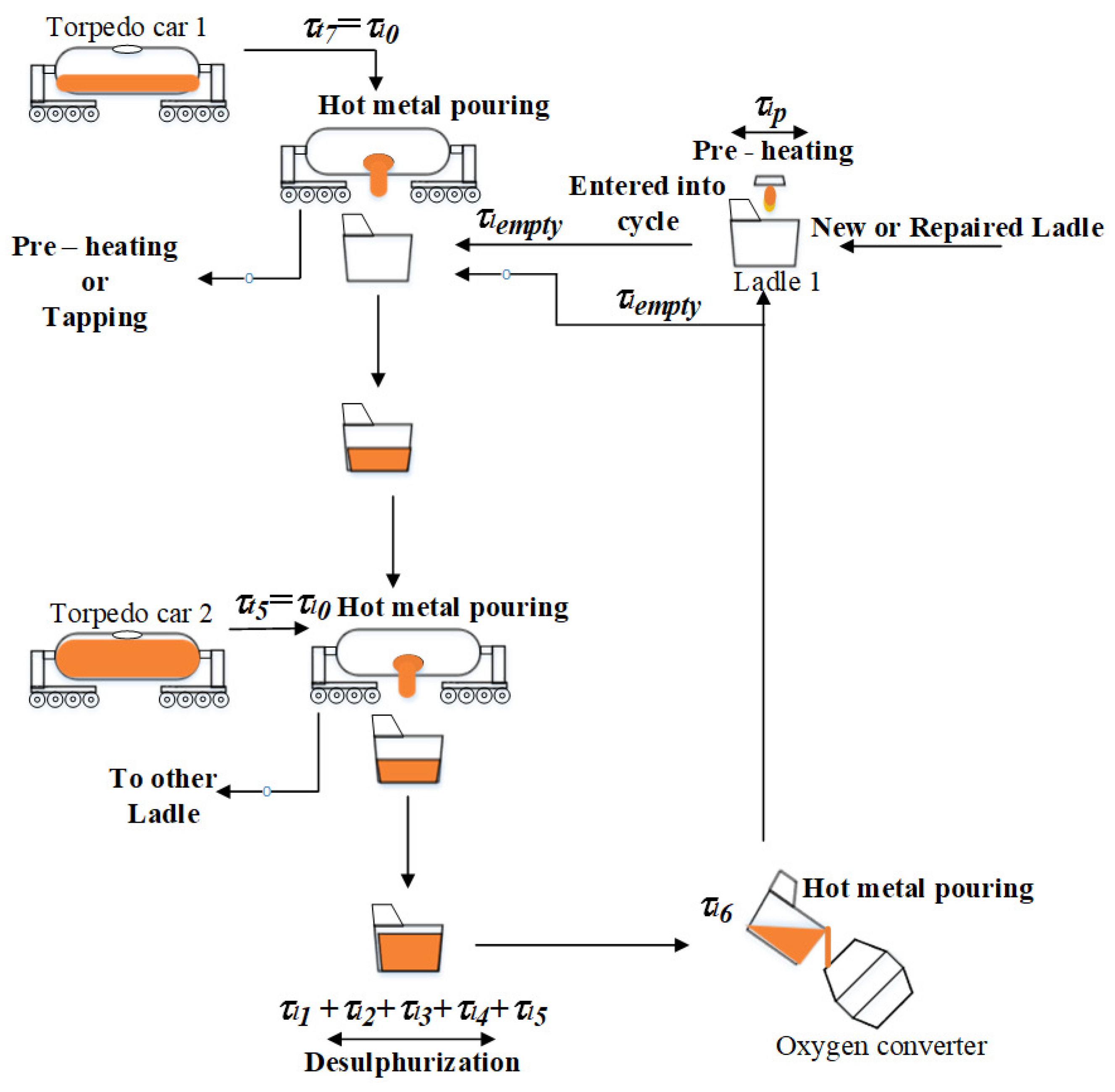
The ladle model must also be supplemented with a pouring function, where the mentioned temperature vector is the input. Furthermore, it was necessary to consider the change in the weight of the poured hot metal and its contact area with the inner wall of the ladle during pouring. The ladle can be poured from several torpedo cars, so it was also necessary to take into account the cooling of the stored hot metal in the ladle between individual pourings (see Figure 2).
Similar to the torpedo car, it was also necessary to solve the problem of pouring the hot metal into the oxygen converter. It was associated with reducing the hot metal weight and its contact area with the inner wall of the ladle. In both models, it was necessary to adjust the thermophysical properties to improve the accuracy of the proposed complex model. A function to calculate the thermal state of the torpedo car and the ladle was added. In case of a low thermal state for these devices, they are recommended for preheating.

2. Materials and Methods

The prediction of hot metal temperature during transport in the torpedo car and the desulfurization in the ladle is solved using the proposal of the mathematical model. The proposed complex model in the form of a mathematical model is based on the co-operation of the heat transfer processes and was implemented in the C# environment.

2.1. Torpedo Car, Ladle, and Hot Metal Description

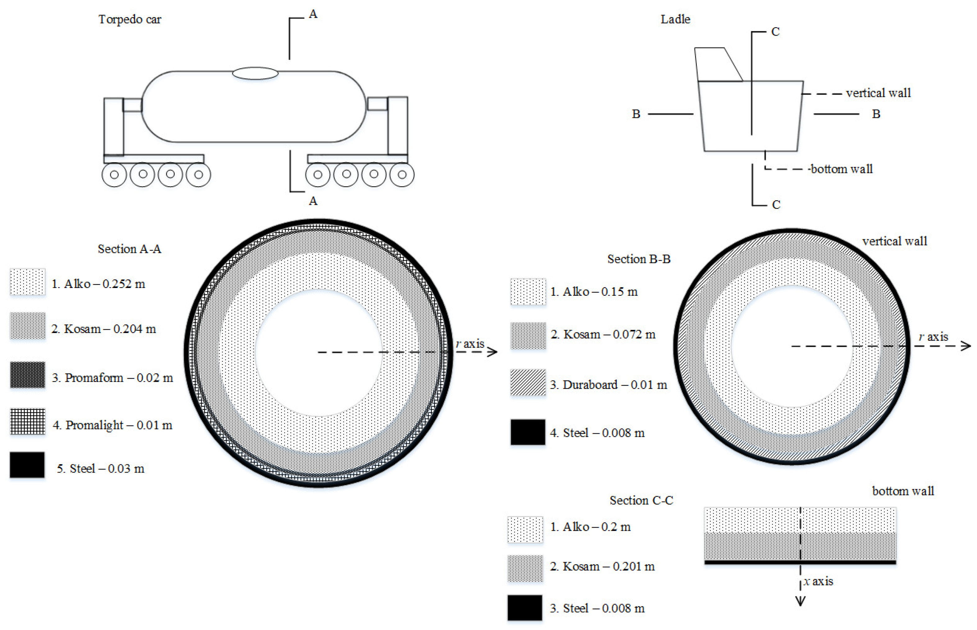
The determination of the count, dimension, and type of wall layers of the torpedo and the ladle was essential for the heat transfer calculation. The individual layers of the torpedo car wall and the ladle walls are shown in Figure 3.
The layers of the torpedo car are shown in section A-A. The torpedo car wall consisted of five layers with the following dimensions (i.e., thickness): 0.252 m for the first layer, 0.204 m for the second layer, 0.02 m for the third layer, 0.01 for the fourth layer, and 0.03 m for the fifth layer (i.e., steel shell).
The distribution of the wall layers in the ladle is different for the vertical and the bottom walls. The layers of the vertical wall are shown in section B-B. The vertical wall consisted of four layers of the following dimensions (i.e., thickness): 0.15 m for the first layer, 0.072 m for the second layer, 0.01 m for the third layer, and 0.008 for the fourth layer (i.e., steel shell). The layers of the bottom wall are shown in section C-C. The bottom wall consisted of three layers of the following dimensions (i.e., thickness): 0.2 m for the first layer, 0.201 m for the second layer, and 0.008 m for the third layer (i.e., steel shell).
Table 1 shows the thermophysical properties (i.e., density ρ , thermal conductivity λ , and heat capacity c) of the torpedo car and ladle wall layers. These properties were obtained from the manufacturer [22,23,24].
The hot metal thermophysical properties, i.e., the density: 6900 kg·m−3, thermal conductivity: 16.5 W·m−1·K−1, heat capacity: 850 J·kg−1·K−1, and emissivity: 0.7, were obtained from the literature [25,26].

2.2. Mathematical Model

Heat conduction, heat convection, heat radiation, heat accumulation, and chemical reactions were considered the main processes affecting the temperature change of the hot metal in the torpedo car and the ladle.

2.2.1. Heat Conduction

Two forms of the heat conduction equation were considered in the proposed mathematical model, i.e., the first form for Cartesian co-ordinates and the second for Polar coordinates [27,28]. The heat conduction equation for one-dimensional transfer in Cartesian co-ordinates has the form
T ( x , τ ) τ = λ ϱ c x T ( x , τ ) x
and in the Polar co-ordinates, it has the form
T ( r , τ ) τ = λ ϱ c 1 r r r T ( r , τ ) r
where T is the temperature (K), τ is the time (s), ϱ is the density (kg·m−3), λ is the thermal conductivity (W·m−1·K−1), c is the specific heat capacity (J·Kg−1·K−1), and x and r are the co-ordinates (m).
After the spatial (i.e., index i) and temporal (i.e., index k) discretizations, the heat conduction equation for Cartesian co-ordinates will have the form
T i k + 1 = λ i , i + 1 ϱ i , i + 1 · c i , i + 1 · ( T i + 1 k T i k ) λ i 1 , i ϱ i 1 , i · c i 1 , i · ( T i k T i 1 k ) Δ x 2 · Δ τ + T i k
and for the Polar co-ordinates, it will have the form
T i k + 1 = λ i , i + 1 ϱ i , i + 1 · c i , i + 1 · r i , i + 1 · T i + 1 k T i k Δ r λ i 1 , i ϱ i 1 , i · c i 1 , i · r i 1 , i · T i k T i 1 k Δ r r i Δ r · Δ τ + T i k
where i = 2 , 3 , , n are the co-ordinates of the calculated inner temperatures, i = 1 is the co-ordinate of the inner object’s surface temperature, i = n + 1 is the co-ordinate of the outer object’s surface temperature, n is the number of wall layers, T i k is the temperatures on the ith co-ordinate at the actual time step k (K), T i k + 1 is the temperatures on the i t h co-ordinate at the next time step k + 1 (K), Δ x (m) is the element size between temperature co-ordinates on the x axis, Δ r (m) is the element size between temperature co-ordinates on the r axis, r i is the distance from of the null value on the r axis to the value on the co-ordinate of the temperature T i (m), r i , i + 1 is the distance from of the null value on the r axis to the value on the position between co-ordinates with temperatures T i and T i + 1 (m), r i 1 , i is the distance from of the null value on the r axis to the value on the position between co-ordinates with temperatures T i 1 and T i (m), and Δ τ (s) is the time step.
The thermal conductivities and the specific heat capacity (see Table 1) were considered the functions of the arithmetic mean of two neighboring temperature points.
The initial condition, i.e., the temperature of the body at time zero, for Cartesian co-ordinates was a function of the axis x co-ordinates T ( x , 0 ) = f ( x ) , and for the Polar co-ordinates, it was a function of the r axis co-ordinates T ( r , 0 ) = f ( r ) .
The Dirichlet boundary condition (the first type of boundary condition), i.e., where the surface temperatures of the object are known variables, was defined as a function of the time T ( 1 , τ ) = f ( τ ) and T ( n + 1 , τ ) = f ( τ ) .
The Neumann boundary condition (the second type of boundary condition), i.e., where the heat flows along the object’s inner and outer surface are known variables, was defined as a function of the time I Q c , 1 ( τ ) = f ( τ ) and I Q c , n + 1 ( τ ) = f ( τ ) .
The Robin boundary condition (the third type of boundary condition), i.e., where the environment temperatures along the object’s inner and outer surface are known variables, was defined as a function of the time T e 1 ( τ ) = f ( τ ) and T e n + 1 ( τ ) = f ( τ ) [28,29].

2.2.2. Heat Convection

The transfer of heat energy using fluid flow is called convection. This transfer can be expressed in the form [30,31]
I Q c ( τ ) = α A ( T 1 ( τ ) T 2 ( τ ) ) .
where I Q c is the heat flow by convection (W), α is the heat transfer coefficient (W·m−2·K−1), A is the area (m2), T 1 is the object’s surface temperature (K), and T 2 is the fluid temperature (K).

2.2.3. Heat Radiation

Heat radiation is the transfer of electromagnetic energy in the form of waves. This transfer between two gray bodies can be expressed in the form [32,33,34]
I Q r ( τ ) = σ A ( T 1 4 ( τ ) T 2 4 ( τ ) ) ϵ 12 ,
where I Q r is the heat flow by radiation (W), T 1 and T 2 are the temperatures of the two gray bodies (K), σ is the Stefan–Boltzmann constant 5.67 × 10⁻⁸ (W·m−2·K−4), A is the area (m2), and ϵ 12 is the resulting emissivity.

2.2.4. Heat Accumulation

Heat accumulation represents a change in heat proportional to a change in temperature per unit of time.
d Q ( τ ) d τ = m c d T ( τ ) d τ .
where Q is the heat (J), c is the specific heat capacity (J·Kg−1·K−1), T is the temperature (K), τ is the time (s), and m is the mass (kg).

2.2.5. Heat of Desulfurization Process

The heat flow via desulfurization was calculated using the reaction heat obtained from considering the chemical reaction and the heat consumed through the heating of the desulfurization mixture components and the nitrogen gas.
I Q d ( τ ) = Δ r H ( T ) M h S m S ( τ ) + l = 1 n C p , l ( T ) M h l m l ( τ ) Δ T ,
where Δ r H ( T ) is the chemical reaction enthalpy at a certain temperature T, m S ( τ ) is the sulfur loss per unit of time (kg·s−1), C p , l is the molar heat capacity of the lth component in the desulfurization mixture (J·Kmol−1·K−1), m l ( τ ) is the mass flow of the lth component in the desulfurization mixture (kg·s−1), M h l is the molar mass of the lth component in the desulfurization mixture (kg·kmol−1), Δ T is the temperature difference between the temperatures of the desulfurization mixture and the hot metal (K), and n is the count of desulfurization mixture components.
The desulfurization mixture contained fluorspar, lime, and magnesium. The reaction of magnesium with sulfur to form magnesium sulfide was considered in the proposed mathematical model.
Mg ( g ) + S ( s ) = MgS ( s ) + Δ r H ( T ) ,

2.3. Implementation

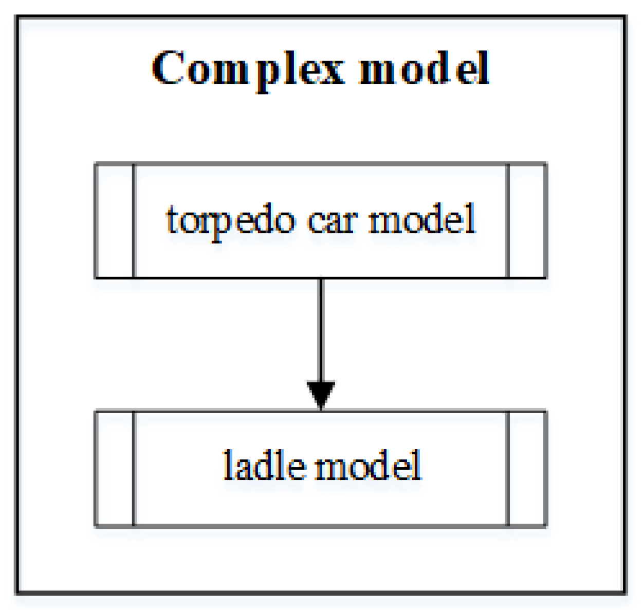
The presented heat transfer, accumulation, and chemical reaction processes were transformed into the complex model (see Figure 4). This complex model included two models, i.e., the first model for the hot metal temperature drop calculation in the torpedo car (torpedo car model) and the second for the hot metal temperature drop calculation in the ladle (ladle model).

2.3.1. Model of the Hot Metal Temperature Drop in the Torpedo Car

The algorithm of the hot metal temperature calculation in the torpedo car is shown in Figure 5. The individual mathematical sub-models were implemented in the C# environment.
Input loading:
The dimensions of the torpedo car, i.e., the inner diameter, inner length, outer diameter, outer length, mass capacity, hole dimension, wall thickness, and wall layer dimensions and thermophysical properties, are set in these models. Subsequently, the torpedo car wall’s temperatures are loaded.
The wall’s heat accumulation model:
The heat accumulated in the torpedo car wall is calculated in this model. The equation for the calculation of this heat is
Q w a l l = i = 1 n ϱ i · V i · c i · T i + 1 + T i 2 293.15
where Q w a l l is the heat accumulated in the torpedo car wall (J), ϱ i is the layer density between T i + 1 and T i temperatures (kg·m−3), V i is the layer volume between T i + 1 and T i temperatures (m3), c i is the layer-specific heat capacity between T i + 1 and T i temperatures (J·kg−1·m−1), 293.15 is the wall’s layer temperature in the cold state (K), T i + 1 and T i are the wall’s layer temperature in the actual state.
Preheating model:
The preheating process starts if a new torpedo enters the process, the wall of the torpedo car is repaired, or the heat accumulated in the torpedo car wall is low. The heat accumulated in the torpedo car wall is compared to the heat accumulated in the torpedo car wall at full charge. The full charge is determined from the wall temperatures calculated using Equation (4) if the maximum temperature of the hot metal on the inner side of the torpedo car wall is considered. The maximum temperature of the hot metal was equal to the maximum tapping temperatures from the blast furnace.
The temperatures inside the wall of the torpedo car during preheating were calculated using Equation (4). The Robin boundary condition was considered in the calculation, i.e., the input variables were the flue gas temperature inside the torpedo car ( T e 1 ( τ ) = T e 1 k ) and the environment temperature outside the torpedo car ( T e n + 1 = T e n + 1 k ). It was assumed that the heat flows along the inner and outer surface of the torpedo car are equal to the heat flow in the torpedo car wall below the surface (i.e., in the boundary elements). The temperature on the inner surface of the torpedo car was determined
α i n n e r · T e 1 k T 1 k · A i n n e r = λ 1 , 2 · r 1 , 2 r 1 · Δ r · T 1 k T 2 k · A i n n e r
T 1 k + 1 = T 1 k = α i n n e r · T e 1 k + λ 1 , 2 · r 1 , 2 r 1 · Δ r · T 2 k α i n n e r + λ 1 , 2 · r 1 , 2 r 1 · Δ r
The temperature on the outer surface of the torpedo car was determined using
λ n , n + 1 · r n , n + 1 r n + 1 · Δ r · T n k T n + 1 k · A o u t e r = α o u t e r · T n + 1 k T e n + 1 k · A o u t e r
T n + 1 k + 1 = T n + 1 k = α o u t e r · T e n + 1 k + λ n , n + 1 · r n , n + 1 r n + 1 · Δ r · T n k α o u t e r + λ n , n + 1 · r n , n + 1 r n + 1 · Δ r
where α i n n e r is the heat transfer coefficient between the flue gas and the inner surface of the torpedo car (W·m−2·K−1) and α o u t e r is the heat transfer coefficient between the outer surface of the torpedo car and the air (W·m−2·K−1).
Torpedo car wall cooling model:
This model simulates the torpedo car’s wall cooling process by calculating the torpedo car wall temperatures if the torpedo car is empty. The torpedo car is in a state between the end of pouring the hot metal into the ladle and the start of the torpedo car preheating or between the end of pouring the hot metal into the ladle and the start of the torpedo car filling.
The temperatures inside the wall of the torpedo car during wall cooling were calculated using Equation (4). The Neumann boundary condition inside the torpedo car was considered, i.e., the heat flow along the inner surface of the wall is known. The Robin boundary condition outside the torpedo car was considered, i.e., the environment temperature outside the torpedo car is known. The temperature on the outer surface of the torpedo car was determined using Equation (13).
It was assumed that the heat flow along the inner surface of the torpedo car is equal to the heat flow below the surface (i.e., in the first element).
I Q i n n e r k = λ 1 , 2 · r 1 , 2 r 1 · Δ r · T 1 k T 2 k · A i n n e r
T 1 k + 1 = T 1 k = I Q i n n e r k A i n n e r + λ 1 , 2 · r 1 , 2 r 1 · Δ r · T 2 k λ 1 , 2 · r 1 , 2 r 1 · Δ r
Here, A i n n e r is the area of the torpedo car inner surface (m2), and I Q i n n e r k is the heat flow between the torpedo car inner surface and the environment through the hole of the torpedo car (W).
The heat flow I Q i n n e r k was determined using the sum of the heat convection (5) flow and heat radiation flow (6). The temperature T 1 ( τ ) is the air temperature, and the temperature T 2 ( τ ) is the temperature T 1 k . Area A is the area of the hole of the torpedo car. The heat transfer coefficient α and emissivity ϵ 12 were determined using the thermophysical properties of the air and the torpedo car wall.
Hot metal weight increase model:
This model is run when hot metal tapping from the blast furnace into the torpedo car is in progress. A torpedo car can be filled during one or more tappings. The hot metal mass is set at the null value (i.e., m H M = 0 ) at the start of tapping. The hot metal mass in the torpedo car is calculated using
m H M = m H M + Δ m H M
where Δ m H M is the increase in mass over time Δ τ (kg).
The change in temperature of the hot metal in the torpedo car during tapping is calculated as
T H M k = m H M · T H M k + Δ m H M · T t a p p i n g k m H M + Δ m H M
where T t a p p i n g k is the hot metal tapping temperature (K), T H M k is the hot metal temperature in the torpedo car, and m H M is the hot metal mass in the torpedo car.
During tapping, the temperature of the hot metal is decreased due to heat losses to the torpedo car wall and the surroundings. The hot metal cooling model calculates these heat losses.
Hot metal cooling model:
This model calculates the drop in hot metal temperature during hot metal tapping, transport, and pouring out. The drop in temperature of the hot metal is caused by heat losses to the wall and the torpedo car’s surroundings
T H M k + 1 = T H M k + Δ τ m H M c H M I Q w k I Q c k I Q r k .
where I Q w is the heat losses into the torpedo car wall (W), I Q c is the heat losses through the torpedo hole at convection heat transfer (W), I Q r is the heat losses through the torpedo hole at radiation heat transfer (W), m H M is the hot metal mass (kg), T H M k is the hot metal temperature at actual time step (K), T H M k + 1 is the hot metal temperature at the next time step (K), c H M is the hot metal specific heat capacity (J·kg−1·K−1), and Δ τ is the time step (s).
The temperature T 1 ( τ ) is the hot metal temperature, and the temperature T 2 ( τ ) is the air temperature at the time of convection (5) and radiation (6) heat loss calculation. The area A is the area of the hole of the torpedo car. The heat transfer coefficient α and emissivity ϵ 12 were determined using the thermophysical properties of the hot metal and the air.
The temperatures in the torpedo wall needed to be determined to calculate the heat losses to the torpedo car wall. The procedure presented in the preheating model section was used for calculating the wall temperatures.
Subsequently, the heat losses to the wall were calculated using Equation (5). The temperature T 1 ( τ ) was the hot metal temperature T H M k , and the temperature T 2 ( τ ) was the inner surface wall temperature T 1 k + 1 . The heat transfer coefficient α was determined using the thermophysical properties of the hot metal. The area A was considered the wall’s inner surface in places where hot metal comes into contact with the wall. The area A is the function of the hot metal volume A = f V H M because the hot metal mass is not constant, i.e., it increases during tapping and decreases during pouring out.
Hot metal weight decrease model:
This model is run when hot metal is poured from the torpedo car into the ladle. The torpedo car is emptied into two or more ladles. The change in the hot metal mass in the torpedo car is calculated
m H M = m H M Δ m H M
where Δ m H M is the decrease in mass over time Δ τ (kg).
Similarly to tapping, the hot metal cooling model calculates heat losses to the torpedo car wall and the surroundings. The temperature of the hot metal is stored in the form of a vector when it is poured into the ladle. This vector contains decreasing values of the hot metal temperature and represents the input values of the hot metal temperature to the ladle model during its filling.
Outputs visualization:
The task of this function is to visualize hot metal temperature behavior using tables and graphs.

2.3.2. Model of the Hot Metal Temperature Drop in the Ladle

The algorithm of the hot metal temperature calculation in the ladle has a similar structure to the one shown in Figure 5, but the ladle is filled with hot metal from the torpedo car. Subsequently, the desulfurization process is carried out in the ladle. After the desulfurization process is completed, the hot metal is poured into the oxygen converter. The individual mathematical sub-models were implemented in the C# environment.
Inputs loading:
The following variables are loaded and set in the ladle model:
  • The ladle mass capacity;
  • The height, the diameter of the pouring hole, and the diameter of the bottom;
  • The vertical and bottom wall layers’ dimensions and thermophysical properties;
  • The temperatures of the vertical wall and the temperatures of the bottom wall;
  • The temperatures of the hot metal poured into the ladle.
Wall heat accumulation model:
The heat accumulated in the ladle walls is calculated using Equation (9) using the dimensions and thermophysical properties of the vertical and bottom ladle walls. The heat accumulated in the ladle is the sum of the heat accumulated in the vertical and bottom walls.
Preheating model:
The preheating process starts if a new ladle enters the process, the walls of the ladle are repaired, or the heat accumulated in the ladle walls is low, similar to the torpedo car. The full charge is determined from the wall temperatures calculated using Equation (3) for the bottom wall and Equation (4) for the vertical wall. The maximum temperature of the hot metal was equal to the maximum poured-out temperatures from the torpedo car.
The temperatures inside the walls of the ladle during preheating were calculated using Equation (3) for the bottom wall and Equation (4) for the vertical wall. Similarly to preheating the torpedo car, Equations (11) and (13) were used for the surface temperature calculations of the vertical wall. The surface temperatures of the bottom wall were determined using the equations expressed for the Cartesian co-ordinates. The temperature on the inner surface of the bottom wall was determined using
α i n n e r · T e 1 k T 1 k · A i n n e r = λ 1 , 2 Δ x · T 1 k T 2 k · A i n n e r
T 1 k = α i n n e r · T e 1 k + λ 1 , 2 Δ x · T 2 k α i n n e r + λ 1 , 2 Δ x
The temperature on the outer surface of the vertical wall was determined using
λ n , n + 1 Δ x · T n k T n + 1 k · A o u t e r = α o u t e r · T n + 1 k T e n + 1 k · A o u t e r
T n + 1 k = α o u t e r · T e n + 1 k + λ n , n + 1 Δ x · T n k α o u t e r + λ n , n + 1 Δ x
where α i n n e r is the heat transfer coefficient between the flue gas and the inner surface of the ladle (W·m−2·K−1), and α o u t e r is the heat transfer coefficient between the outer surface of the ladle and the air (W·m−2·K−1).
Ladle wall cooling model:
This model simulates the ladle’s wall cooling process by calculating the ladle walls’ temperatures if the ladle is empty. The ladle is in a state between the end of pouring the hot metal into the oxygen converter and the start of ladle preheating or between the end of pouring the hot metal into the oxygen converter and the start of ladle filling.
The temperatures inside the vertical wall were calculated using Equation (4), and those inside the bottom wall were calculated using Equation (3) during wall cooling. Equations (15) and (13) were used for the vertical wall surface temperature. The temperature on the outer surface of the bottom wall was determined using Equation (23). The temperature on the inner surface of the bottom wall was calculated as
I Q i n n e r k = λ 1 , 2 Δ x · T 1 k T 2 k · A i n n e r
T 1 k + 1 = T 1 k = I Q i n n e r k A i n n e r + λ 1 , 2 Δ x · T 2 k λ 1 , 2 Δ x
where A i n n e r is the area of the bottom wall’s inner surface (m2), and I Q i n n e r k is the heat flow between the bottom wall’s inner surface and the environment through the pouring hole of the ladle (W).
The heat flow I Q i n n e r k was determined using the sum of the heat convection (5) flow and heat radiation flow (6).
Hot metal weight increase model:
This model is run when the hot metal is poured from the torpedo car into the ladle. The ladle can be filled in sequence from one or more of the torpedo cars. At the start of pouring, the hot metal mass in the ladle is set at the null value (i.e., m H M = 0 ). The hot metal mass in the ladle is calculated using Equation (16), and Δ m H M is the increase in mass over time Δ τ . The hot metal temperature T H M , p decreases via the convection (5) and radiation (6) heat losses into the environment during pouring:
T H M , p k = T H M , p k I Q c + I Q r Δ m H M · c H M · Δ τ
Subsequently, the change in temperature of the hot metal in the ladle during pouring is calculated using Equation (16). The hot metal tapping temperature in this equation is replaced by the temperature of the hot metal poured out from the torpedo car.
Hot metal cooling model:
The hot metal temperature at the next time step is calculated similarly to Equation (18), but the heat from the chemical reaction process I Q d (determined by Equation (7)) must also be considered:
T H M k + 1 = T H M k + Δ τ m H M c H M I Q w k I Q c k I Q r k I Q d k .
Similar to the calculation of the heat losses to the torpedo wall, temperatures in the vertical and bottom ladle walls need to be determined. The wall temperatures were calculated using the procedure described in the preheating model section. Subsequently, two amounts of heat losses to the wall were calculated using Equation (5) and summed, with the first used for the vertical wall and the second for the bottom wall. Area A is the function of the hot metal volume A = f V H M .
Hot metal weight decrease model:
This model runs when the hot metal is poured into the oxygen converter from the ladle. Equation (19) calculates the change in the hot metal mass in the ladle.
Similarly to pouring into the ladle, the hot metal cooling model calculates the heat losses to the ladle walls and the surroundings. The temperature of the hot metal is stored in the form of a vector when it is being poured into the oxygen converter. This vector contains decreasing values for the hot metal temperature and represents the input values of the hot metal temperature to the next steelmaking process in the oxygen converter.
Output visualization:
Similar to the torpedo car, this function visualizes the hot metal temperature behavior using tables and graphs.

3. Results and Discussion

The proposed complex model for predicting the temperature of hot metal in a torpedo car and ladle was verified using measured data from the real operation. The measured data were obtained from the measuring sensors and stored in the information system. Subsequently, the data were exported to us in table form for the verification of the proposed model. The simulation model created in the C# environment was used for verification. First, a sensitivity analysis was used to assess the impact of heat losses on the change in the temperature of the hot metal. The results of the sensitivity analysis were used to estimate the model parameters. Subsequently, simulations using these parameters were performed, and errors in the calculations were determined.

3.1. Input Data

The data from the three torpedo cars with 350 t capacity and the nine ladles with 150 t capacity were used for the simulation. The mass of the hot metal was poured from the torpedo car into two ladles in these simulations. The measured data were obtained from nine operating cycles (see Table 2).
These measured data from the torpedo cars were used for the simulation (see Table 3): the weight of the hot metal from the first tapping m t a p 1 , the weight of the hot metal from the second tapping m t a p 2 , the tapping temperatures of the hot metal (the first tapping, i.e., T t a p 11 , T t a p 12 , and T t a p 13 and the second tapping, i.e., T t a p 21 , T t a p 22 , and T t a p 23 ), the measurement time (i.e., format hh:mm:ss) of the tapping temperatures, the period of time when the torpedo car was empty τ t e m p t y , the time taken between the start and end of pouring out into the first ladle (i.e., format: hh:mm:ss), the time taken between the start and end of pouring out into the second ladle (i.e., format: hh:mm:ss), the hot metal weight for the first ladle m 1 , and the hot metal weight for the second ladle m 2 . The time data were used for the time calculations.
The first period τ t 1 is defined as being from the start to the end of the first tapping. The second period τ t 2 is defined as being from the end of the first tapping to the start of the second tapping. The third period τ t 3 is defined as being from the start of the second tapping to the end of the second tapping. The fourth period τ t 4 is defined as being from the end of the second tapping to the start of pouring the hot metal into the first ladle. The fifth period τ t 5 is defined as being from the start to the end of pouring hot metal into the first ladle. The sixth period τ t 6 is defined as being from the end of the pouring the hot metal into the first ladle to the start of the pouring the hot metal into the second ladle. The seventh period τ t 7 is defined as being from the start to the end of the pouring the hot metal into the second ladle. If the torpedo car is filled only from one tapping, the periods τ t 2 and τ t 3 are equal null values, and period τ t 4 is defined as being from the end of the first tapping to the start of pouring the hot metal into the first ladle.
These measured data from the ladles were used for the simulation (see Table 4 and Table 5): the temperature of the hot metal before the desulfurization process in the ladle T 1 , the temperature of the hot metal after the desulfurization process in the ladle T 2 , the weight of the hot metal before the desulfurization process m 1 , the weight of the hot metal after the desulfurization process m 2 , the weight of the desulfurization mixture m z , the nitrogen volume V N 2 , the time of the ladle being empty τ l e m p t y , the sulfur concentration in the hot metal before the desulfurization process S 0 , and the sulfur concentration in the hot metal after the desulfurization process S k . The values of the measured temperatures T 1 and T 2 were obtained from real operations during the processes carried out in the ladle. Taking a sample of the hot metal and measuring the temperature T 1 is realized after inserting the ladle into the box. The amount of the desulfurization mixture is determined using the composition of the hot metal. Subsequently, the desulfurization process is realized. Taking a sample and a temperature T 2 measurement is realized if the desulfurization process is completed and the slag is withdrawn [21].
The time data measured in the ladle were used for the time calculations. The first period is from the end of pouring hot metal into the ladle to placing the ladle in the box τ l 1 . The second period is from putting the ladle in the box to the start of the desulfurization mixture injection τ l 2 . The third period is from the time of the start to the end of the injection τ l 3 . The fourth period is from the end of injection to the time of removal from the box τ l 4 . The fifth period is for slag removal τ l 5 . The sixth period is from the end of slag removal to pouring hot metal from the ladle into the oxygen converter τ l 6 . The period τ l 0 is the time taken pouring hot metal from the torpedo car into the ladle. In the case of filling the ladle from two torpedo cars, this period τ l 0 must include the time period for pouring the hot metal from the first torpedo into the ladle, pouring the hot metal from the second torpedo into the ladle, and cooling the hot metal between these two time periods.
The model includes six different time periods in which the heat transfer coefficients and emissivity coefficient were determined.

3.2. Sensitivity Analysis

Sensitivity analysis was performed on data from the fourth operating cycle. First, a simulation was performed with the assumed values of the model parameters. The simulation results are shown in Table 6. This table illustrates the difference between measured and simulated temperatures in the range of 39 to 47 °C. The model temperature is significantly lower than the measured one, i.e., the calculated heat losses in the complex model are higher than the real heat losses. For this reason, we focused on increasing the accuracy of the heat loss calculation.
The aim of the sensitivity analysis was to determine those heat losses (i.e., at radiation and convection heat transfer) with the most significant impact on the changes in temperature of the calculated temperatures T 1 and T 2 . The difference between the measured and calculated temperatures for T 1 and T 2 should be minimal. The temperature changes were determined after setting the individual heat losses to the null value. The heat transfer coefficient α was set to the null value for convection. For radiation, the resulting emissivity parameter ε 12 was set to the null value. The individual regimes were evaluated, i.e., first, the empty and full torpedo car and, subsequently, the empty and full ladle.
The simulations were performed using the null values of the individual heat losses. The changes in temperature of the temperatures T 1 and T 2 between the simulations with the assumed model parameters and the heat losses set to the null state were determined.

3.2.1. Torpedo Car Model Sensitivity Analysis

For the torpedo car, the following values of the model parameters (i.e., the heat losses) were changed:
1.
The regime of the empty torpedo car was evaluated. The heat transfer coefficient α , i.e., between the inner surface of the torpedo car wall and the air, was set to the null value.
2.
The regime of the full torpedo car was evaluated. The heat transfer coefficient α , i.e., between the hot metal and the air, was set to the null value.
3.
The regime of the full torpedo car was evaluated. The heat transfer coefficient α , i.e., between the hot metal and the inner surface of the torpedo car wall, was set to the null value.
4.
The regime of the empty and full torpedo car was evaluated. The heat transfer coefficient α , i.e., between the outer surface of the torpedo car wall and the air, was set to the null value.
5.
The regime of the empty torpedo car was evaluated. The resulting emissivity coefficient ε 12 , i.e., between the inner surface of the torpedo car wall and the air, was set to the null value.
6.
The regime of the full torpedo car was evaluated. The resulting emissivity coefficient ε 12 , i.e., between the hot metal and the air, was set to the null value.
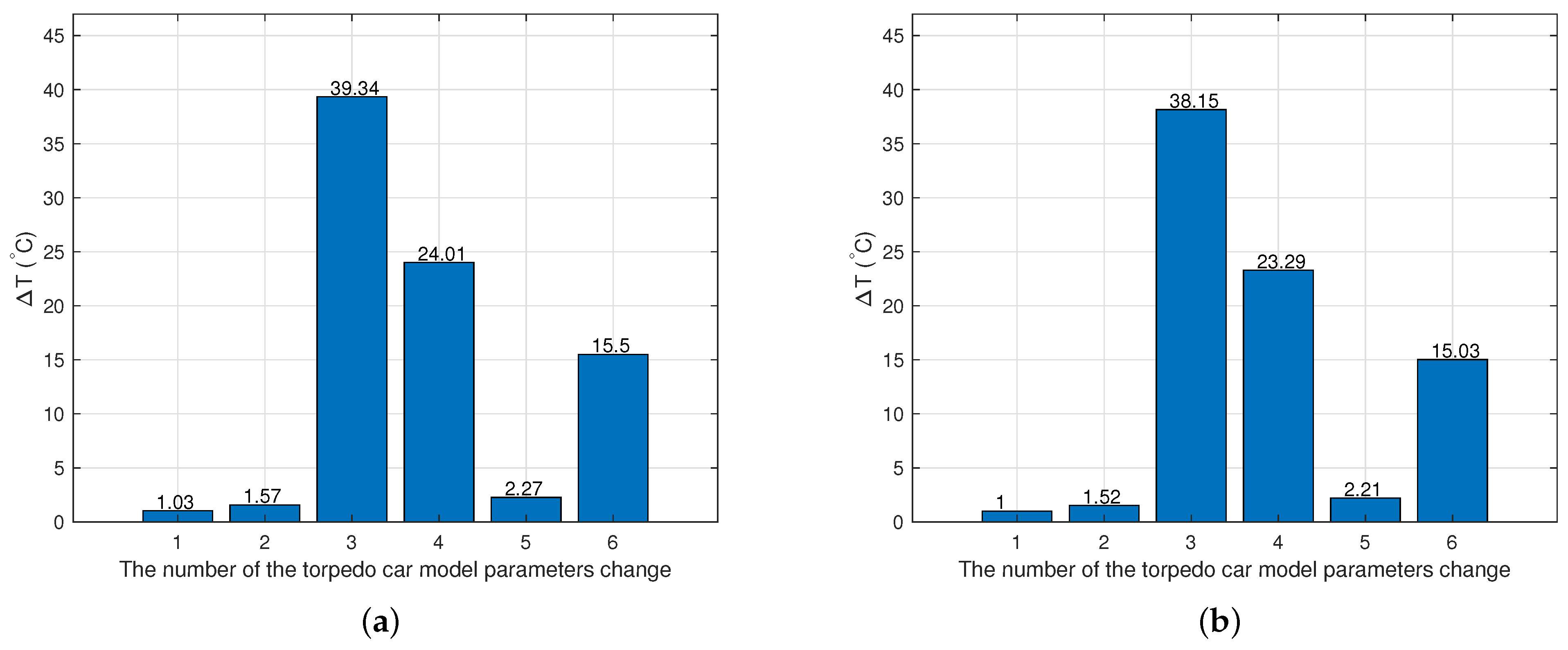
The results of the sensitivity analysis for the individual changes in the torpedo car model parameters are shown in Figure 6 for the first ladle and Figure 7 for the second ladle. These figures represent the temperature increase of the modeled temperature shown in Table 6 after setting the individual heat losses to the null value. For example, the value 39.34 shown in Figure 6a represents an increase in the modeled temperature T 1 m o d e l e d in the first ladle (1344.68 °C) by 39.34 °C after setting the heat transfer coefficient between the hot metal and the inner surface of the torpedo car wall to the null value. The value of the modeled temperature T 1 m o d e l e d is 1384.02 °C after this simulation.
The results show that the following model parameters in the torpedo car model have the most significant impact on the change in the modeled temperatures: the heat transfer coefficient between the hot metal and the wall, i.e., heat losses into the wall of the torpedo car; the heat transfer coefficient between the outer surface of the torpedo car and the air, i.e., heat losses from the outer surface of the torpedo car to the environment; the resulting emissivity coefficient between the hot metal and the air, i.e., heat losses from the hot metal to the environment.

3.2.2. Ladle Model Sensitivity Analysis

For the ladle, the following values of the model parameters (i.e., the heat losses) were changed:
1.
The time period τ l 0 in the ladle was evaluated. The resulting emissivity coefficient ε 12 , i.e., between the hot metal and the air, was set to the null value.
2.
The time period τ l e m p t y was evaluated. The resulting emissivity coefficient ε 12 , i.e., between the inner surface of the ladle wall and the air, was set to the null value.
3.
The time period τ l 1 was evaluated. The heat transfer coefficient α , i.e., between the hot metal and the air, was set to the null value.
4.
The time period τ l 1 was evaluated. The resulting emissivity coefficient ε 12 , i.e., between the hot metal and the air, was set to the null value.
5.
The time period τ l 2 was evaluated. The heat transfer coefficient α , i.e., between the hot metal and the air, was set to the null value.
6.
The time period τ l 3 was evaluated. The heat transfer coefficient α , i.e., between the hot metal and the air, was set to the null value.
7.
The time period τ l 5 was evaluated. The heat transfer coefficient α , i.e., between the hot metal and the air, was set to the null value.
8.
The time period τ l 5 was evaluated. The resulting emissivity coefficient ε 12 , i.e., between the hot metal and the air, was set to the null value.
9.
The time period τ l 6 was evaluated. The resulting emissivity coefficient ε 12 , i.e., between the hot metal and the air, was set to the null value.
10.
All the time periods at the full ladle were evaluated. The heat transfer coefficient α , i.e., between the hot metal and the inner surface of the ladle, was set to the null value.
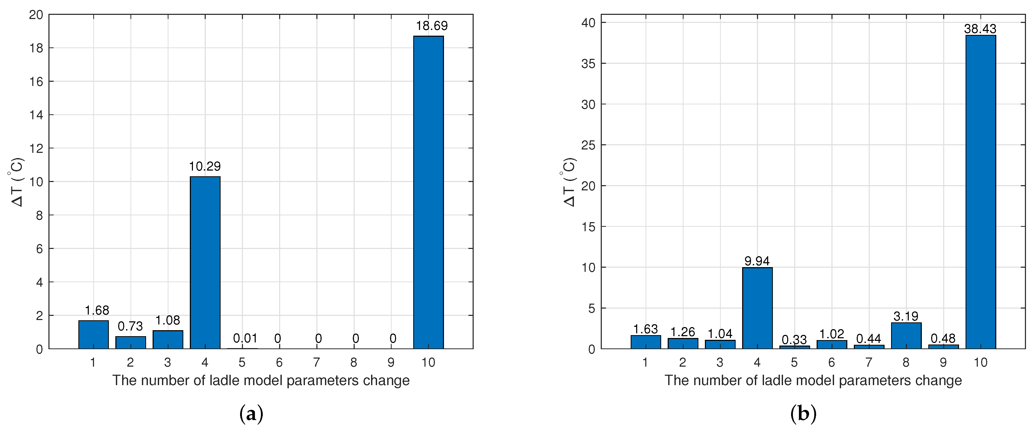
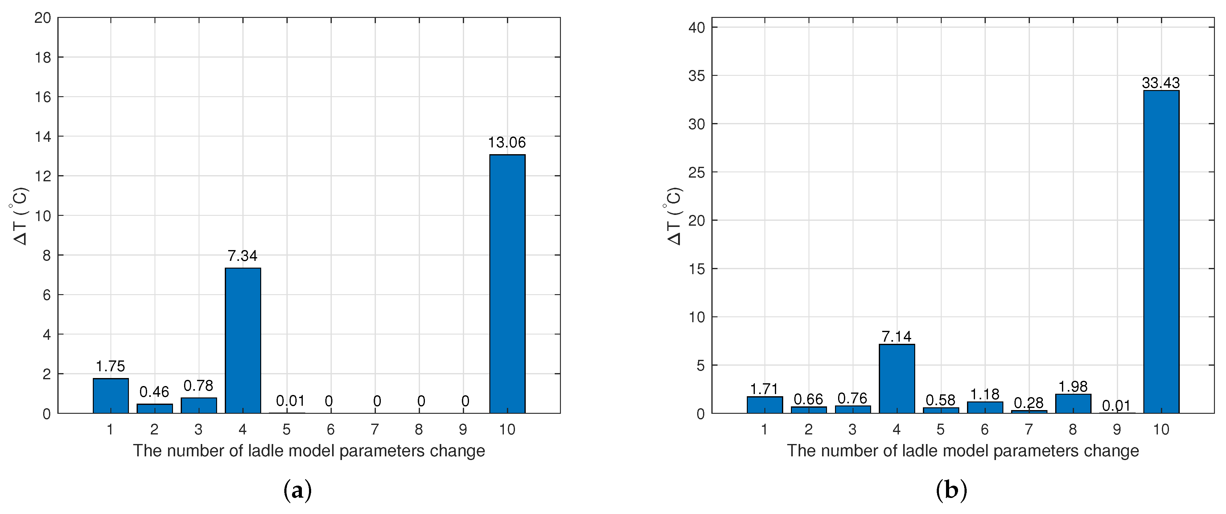
The results of the sensitivity analysis for the individual changes in the ladle model parameters are shown in Figure 8 for the first ladle and Figure 9 for the second ladle. From these figures, it can be seen that the following parameters in the ladle model have the most significant impact on the change in the modeled temperatures: ε 12 when pouring the hot metal from the torpedo car into the ladle (i.e., time period τ l 0 ), i.e., heat losses from the hot metal to the environment; α and ε 12 before placing the ladle into the box (i.e., time period τ l 1 ), i.e., heat losses from the hot metal to the environment; α at the time of injection (i.e., time period τ l 3 ), where the impact is on the temperature T 2 , i.e., heat losses from the hot metal to the environment; α between the hot metal and the inner surface of the ladle through all the time periods, i.e., heat losses into the ladle wall, where the most significant impact is on the temperature T 2 ; ε 12 at the slag removal (i.e., time period τ l 5 ), where the impact is on the temperature T 2 , i.e., heat losses from the hot metal to the environment.
The heat losses into the wall were subjected to further analysis. This analysis showed significant changes in the modeled temperature if the value α between the hot metal and the inner surface of the ladle was lower than 100. This value is significantly lower than what is reported in the literature for the contact of hot metal with the wall. For this reason, this parameter was excluded from the model parameter adjustments to increase the accuracy of the complex model.

3.3. Complex Model Verification

The heat losses from the outer surface of the torpedo car to the environment (i.e., the change in the fourth model parameter in the torpedo car sensitivity analysis), the heat losses from the hot metal stored in the torpedo car to the environment (i.e., the change in the sixth model parameter in the torpedo car sensitivity analysis), and the heat losses from the hot metal stored in the ladle to the environment (i.e., the change in the fourth model parameter in the ladle sensitivity analysis) were estimated to minimize the difference between the measured and modeled temperatures T 1 .
The reduction in these heat losses was needed because the modeled temperature T 1 was lower than the measured temperature T 1 (see Table 6). A significant decrease in the heat losses from the outer surface of the torpedo car to the environment was reached using the application of a reduction coefficient of 1/8. For the losses from the hot metal to the environment, the same reduction coefficient of 1/2.4 was estimated for the process in the torpedo car and also the ladle.
The heat losses from the hot metal stored in the ladle to the environment (i.e., the change in the eighth model parameter in the ladle sensitivity analysis) were estimated to minimize the difference between the measured and modeled temperatures T 2 . The change in heat losses during the slag removal time period only affects temperature T 2 because this time period occurs after temperature T 1 has been measured. The difference between the measured and modeled temperatures T 2 was reduced by the applied reduction coefficient of 1/1.125 for these heat losses.
The relevant heat transfer and resulting emissivity coefficients were multiplied by the estimated reduction coefficients. These are the values of some of the model parameters used in the complex model:
  • The heat transfer coefficient between the hot metal and the inner surface of the torpedo car wall, i.e., α = 1062.8 W·m−2·K−1 at the temperature 1350 °C.
  • The heat transfer coefficient between the outer surface of the torpedo car and the air, i.e., α = 3.89 W·m−2·K−1 at the temperature 200 °C.
  • The resulting emissivity coefficient between the hot metal stored in the torpedo car and the air, i.e., ε 12 = 0.17 .
  • The resulting emissivity coefficient between the hot metal stored in the ladle and the air before placing the ladle into the box (i.e., time period τ l 1 ), i.e., ε 12 = 0.17 .
  • The heat transfer coefficient between the hot metal and the inner surface of the ladle through all the time periods, i.e., α = 1062.8 W·m−2·K−1 at the temperature 1350 °C.
  • The resulting emissivity coefficient between the hot metal stored in the ladle and the air during the slag removal (i.e., time period τ l 5 ), i.e., ε 12 = 0.33 .
After the set parameters were modeled, verification using data from nine operating cycles was realized. The calculation of the absolute and relative errors was used for the verification process. The absolute and relative errors were calculated between the measured and modeled temperatures, i.e., measured and modeled temperature T 1 and measured and modeled temperature T 2 . The absolute error is
Δ T = | T m e a s u r e d T m o d e l e d |
and the relative error is
δ T = Δ T T m e a s u r e d · 100
The average relative error was calculated using the relative errors of the nine operating measurements.
δ T ¯ = i = 1 9 δ T i 9
The calculated values of the absolute and relative errors for individual operating cycles are shown in Table 7 for the first ladle and in Table 8 for the second ladle. Table 7 shows that after setting the model parameters, the relative error values for the first ladle are in the range of 0.276 to 1.861% for temperature T 1 and 0.380 to 1.922% for temperature T 2 . The absolute error values for the first ladle are in the range of 3.92 to 25.63 °C for temperature T 1 and 5.22 to 26.43 °C for temperature T 2 . Table 8 shows that the relative error values for the second ladle are in the range of 0.005 to 2.351% for temperature T 1 and in the range of 0.246 to 2.371% for temperature T 2 . The absolute error values for the second ladle are in the range of 0.06 to 31.31 °C for temperature T 1 and 3.27 to 32.49 °C for temperature T 2 .
The most significant relative error appears in the third operational measurement, where the highest tapping temperatures were measured. At these temperatures, there was a higher hot metal temperature drop than that calculated by the model. This error may be due to the incorrect determination of the thermal charge of the torpedo car or ladle.
The most significant error in the second operating measurement is determined at the temperature T 2 in the second ladle. In this operating measurement, the longest time occurs from the end of injection to the beginning of slag removal. This time could have affected the calculation in the case of inaccurate determination of the model parameters in this time period τ l 4 .
The average relative error for the first ladle is 0.958% for temperature T 1 and 1.008% for temperature T 2 . The average relative error for the second ladle is 0.873% for temperature T 1 and 1.145% for temperature T 2 .
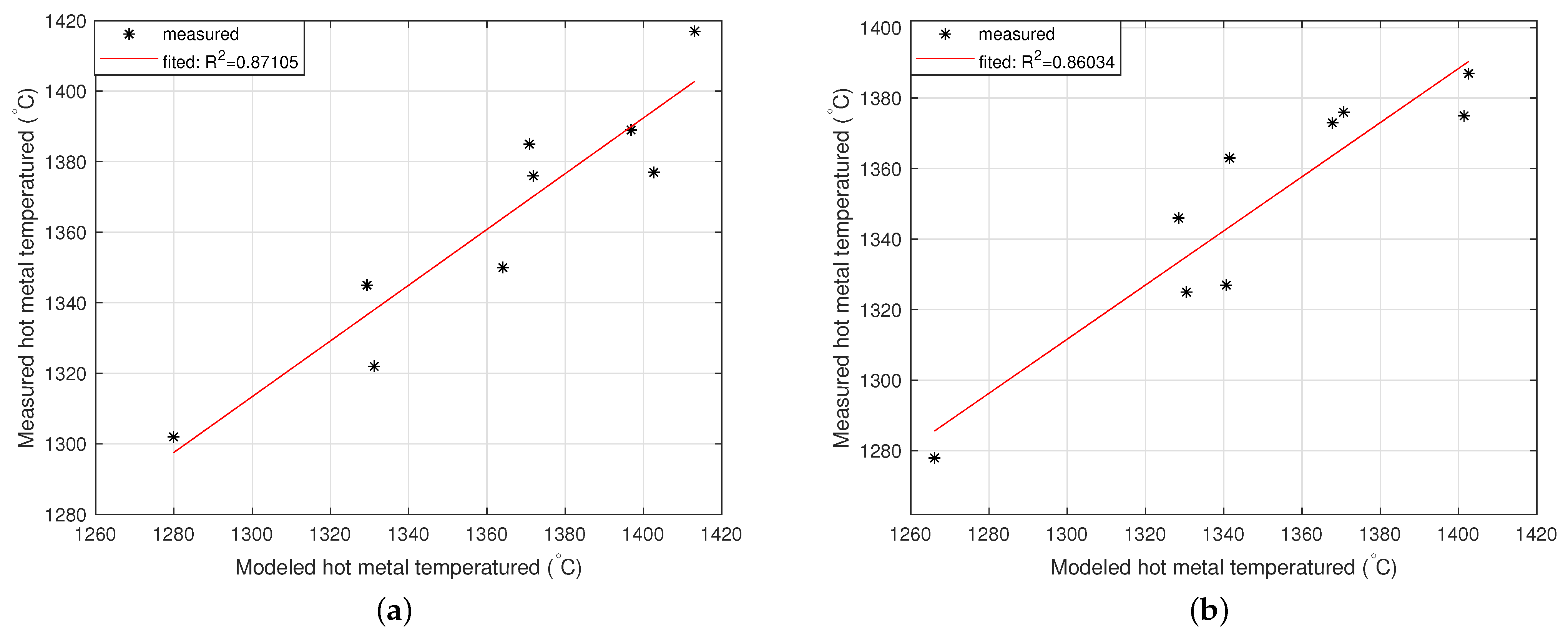
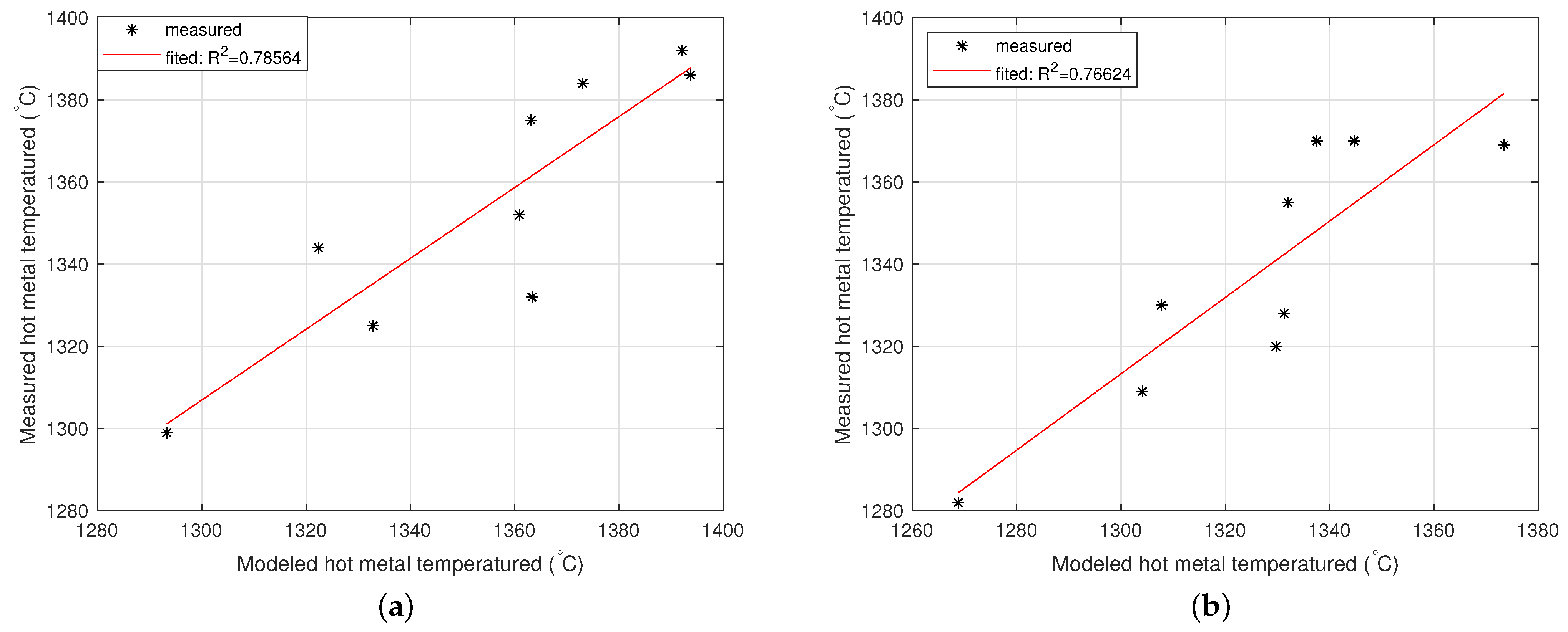
The correlation between the measured and modeled hot metal temperature before desulfurization T 1 and after desulfurization T 2 in the first ladle is shown in Figure 10. The correlation coefficient has a value of 0.87105 for the T 1 temperature and 0.86034 for T 2 . The correlation between the measured and modeled hot metal temperatures before desulfurization T 1 and after desulfurization T 2 in the second ladle is shown in Figure 11. The correlation coefficient has a value of 0.78564 for the T 1 temperature and 0.76624 for T 2 . Lower values of the correlation coefficient in the simulations on the second ladle correspond to a higher range between the minimum and maximum value of the relative error.
These presented errors can also be caused by an inaccurately determined thermal state of the torpedo car and the ladle at the beginning of the process. Suppose the calculation does not start with preheating but is applied to the torpedo car or ladle that is in the cycle. In that case, it is necessary to determine the initial thermal state of the torpedo car and the ladle based on the selected number of previous cycles.
  • In the case of the torpedo car, the inputs are the measured tapping temperatures and the assumed thermal state obtained using the torpedo preheating model. Subsequently, using the selected cycles, the thermal state of the torpedo car is calculated using the torpedo model applied to these cycles [20].
  • In the case of the ladle, the inputs are the measured temperature T 1 and the assumed thermal state obtained using the ladle preheating model. Subsequently, by using the selected cycles, the thermal state of the ladle is calculated using the ladle model applied to these cycles [21].

4. Conclusions

This article presents a complex model for predicting the drop in hot metal temperature in a torpedo car and ladle. The novelty of the presented approach lies in calculating the hot metal temperature between the start of the hot metal pouring from the blast furnace into the torpedo car and the end of the hot metal pouring from the ladle into the oxygen converter. This model is able to calculate the temperature of the hot metal using the values of the measured tapping temperatures, the weight of the hot metal, the weight of the desulfurization mixture, the volume of nitrogen, the torpedo car thermal state, the ladle thermal state, and individual time periods. The output, in addition to the calculated temperature of the hot metal, is the determined thermal states of the torpedo car and the ladle.
The torpedo car model sensitivity analysis showed which of the model parameters had the most significant impact on the change in hot metal temperature in the torpedo car, i.e., the heat transfer coefficient from the outer surface of the torpedo car to the environment and the resulting emissivity from the hot metal to the environment.
The ladle model sensitivity analysis showed those model parameters with the most significant impact on the change in hot metal temperature in the ladle, i.e., the resulting emissivity and heat transfer coefficient from the hot metal to the environment and the heat transfer coefficient in the injection time of the desulfurization mixture.
The complex model verification showed that, for individual temperatures measured in the ladle, the relative error ranges from 0.005 to 2.371%, and the absolute error ranges from 0.06 to 32.49 °C. The correlation coefficient ranges from 0.76624 to 0.87105. The frequency of the relative errors is 94.44% under 2% of the relative error, 72.22% under 1.5% of the relative error, and 52.77% under 1% of the relative error. The values of the average relative error range from 0.873 to 1.145%, which confirms that the proposed model could be used for the hot metal temperature prediction in a torpedo car and ladle with sufficient accuracy.
The proposed model can be utilized for monitoring hot metal temperatures, analyzing the linings’ influence on hot metal transport in terms of heat accumulation, investigating the desulfurization process, and optimizing torpedo and ladle selection based on accumulated heat.

Author Contributions

Conceptualization, M.D., J.T. and G.T.; Data curation, P.F., M.L. and G.T.; Formal analysis, M.D. and J.T.; Methodology, M.D. and J.T.; Project administration, J.K.; Resources, M.D., P.F. and J.K.; Supervision, M.D. and G.T.; Validation, M.D., J.T. and M.L.; Writing—Original draft preparation, M.D., J.T., M.L. and J.K. All authors have read and agreed to the published version of the manuscript.

Funding

This work was supported by the Slovak Research and Development Agency under the contract No. APVV-18-0526, APVV-22-0508, and by the contract on the co-operation in research and development between the Technical University of Košice and the U.S. Steel Košice.

Data Availability Statement

The original contributions presented in this study are included in the article. Further inquiries can be directed to the corresponding author.

Acknowledgments

We appreciate the support from the Slovak Research and Development Agency under the contract No. APVV-18-0526, APVV-22-0508 and from the contract on the co-operation in research and development between the Technical University of Košice and the U.S. Steel Košice.

Conflicts of Interest

Author Gabriel Tréfa was employed by the company U.S. Steel Košice s.r.o. The remaining authors declare that the research was conducted in the absence of any commercial or financial relationships that could be construed as a potential conflict of interest.

References

  1. Shen, Z.; Han, W.; Hu, Y.; Zhu, Y.; Han, J. An Interpretable Hybrid Deep Learning Model for Molten Iron Temperature Prediction at the Iron-Steel Interface Based on Bi-LSTM and Transformer. Mathematics 2025, 13, 975. [Google Scholar] [CrossRef]
  2. Chen, W.; Hu, H.; Wang, S.; Chen, F.; Guo, Y.; Yang, L. Numerical Study on Heat Transfer Characteristic of Hot Metal Transportation before EAF Steelmaking Process. Metals 2024, 14, 673. [Google Scholar] [CrossRef]
  3. Zhao, J.; Zang, Y.; Qin, Q.; Wu, D. Thermo-mechanical Analysis of Torpedo Car. Appl. Mech. Mater. 2011, 44–47, 1198–1202. [Google Scholar] [CrossRef]
  4. Verdeja-Gonzalez, L.; Barbes-Fernandez, M.; Gonzalez-Ojeda, R.; Castillo, G.; Colas, R. Thermal Modelling of a Torpedo-car. Rev. Metal. 2005, 41, 449–455. [Google Scholar] [CrossRef]
  5. Song, X.; Meng, Y.; Liu, C.; Yang, Y.; Song, D. Prediction of Molten Iron Temperature in the Transportation Process of Torpedo Car. ISIJ Int. 2021, 61, 1899–1907. [Google Scholar] [CrossRef]
  6. Diaz, J.; Javier Fernandez, F.; Manuela Prieto, M. Hot Metal Temperature Forecasting at Steel Plant Using Multivariate Adaptive Regression Splines. Metals 2020, 10, 41. [Google Scholar] [CrossRef]
  7. Niedringhaus, J.; Blattner, J.; Engel, R. Armco’s Experimental 184 mile Hot Metal Shipment. In Proceedings of the Ironmaking Conference Proceedings; Iron & Steel Society: Ann Arbor, MI, USA, 1988; pp. 1–5. [Google Scholar]
  8. Tang, Y.; Liu, K. Online Monitoring of Torpedo Car Shells Based on Equal Angle Scanning. Appl. Sci. 2021, 11, 8053. [Google Scholar] [CrossRef]
  9. Botelho, R.; Calente, A. On-line Monitoring of Torpedo Car Shells. In Proceedings of the Thermosense XXIII, Proceedings of the Society of Photo-Optical Instrumentation Engineers (SPIE), Orlando, FL, USA, 16–19 April 2001; Volume 4360, pp. 277–284. [Google Scholar] [CrossRef]
  10. Jin, S.; Harmuth, H.; Gruber, D.; Buhr, A.; Sinnema, S.; Rebouillat, L. Thermomechanical Modelling of a Torpedo Car by Considering Working Lining Spalling. Ironmak. Steelmak. 2020, 47, 145–149. [Google Scholar] [CrossRef]
  11. Ochoterena, L.; Reyes, F.; Ingalls, A.; Gutiérrez, J.; Plascencia, G. Mass Transfer Kinetics in the Desulphurisation of Pig Iron with CaO and CaC2. Defect Diffus. Forum 2008, 273–276, 485–490. [Google Scholar] [CrossRef]
  12. Brodrick, C. Desulphurization of pig iron using calcium carbide based reagents. In Proceedings of the 7th International Heavy Minerals Conference `What next’, The Southern African Institute of Mining and Metallurgy, Drakensberg, South Africa, 20–23 September 2009; pp. 141–146. [Google Scholar]
  13. Shevchenko, A.F.; Vergun, A.S.; Bulakhtin, A.S.; Shevchenko, S.A.; Kislyakov, V.G. Improving the ladle desulfurization of hot metal in low-sulfur steel production. Steel Transl. 2011, 41, 996–998. [Google Scholar] [CrossRef]
  14. Doschek-Held, K.; Krammer, A.C.; Steindl, F.R.; Gatschlhofer, C.; Raonic, Z.; Wohlmuth, D. Treatment of Metallurgical Residues by Chemical Modification, Reduction, and Phase Modification for Metal Recovery and Slag Utilization. Minerals 2025, 15, 408. [Google Scholar] [CrossRef]
  15. Mahendra, K.C.; Gouda, H.V.; Adarsha, K.; Muniswami, K.; Kurubara, H.; Shivaraj, R.N. Hot Metal De-Sulphurisation by KR Process. Int. J. Res. Appl. Sci. Eng. Technol. 2017, 5, 1556–1565. [Google Scholar]
  16. Rodríguez, Y.C.; Múzquiz, G.G.; Torres, J.R.P.; Vidaurri, L.E.R. Mathematical Model of Hot Metal Desulfurization by Powder Injection. Adv. Mater. Sci. Eng. 2012, 2012, 1–5. [Google Scholar] [CrossRef]
  17. Grillo, F.F.; de Alcantara Sampaio, R.; Viana, J.F.; Espinosa, D.C.R.; de Oliveira, J.R. Analysis of pig iron desulfurization with mixtures from the CaO-Fluorspar and CaO-Sodalite system with the use of computational thermodynamics. REM Rev. Esc. Minas 2013, 66, 461–465. [Google Scholar] [CrossRef]
  18. Viertauer, A.; Trummer, B.; Dott, K.H.; Spiess, B.; Hackl, G.; Skala, K.; Pellegrino, M. Efficient Hot Metal Desulphurization Ladle. In Proceedings of the 14th International Symposium on the Desulfurization of Hot Metal and Steel, Athens, Greece, 14–17 September 2016; pp. 1–3. [Google Scholar]
  19. Farrera-Buenrostro, J.E.; Hernández-Bocanegra, C.A.; Ramos-Banderas, J.A.; Torres-Alonso, E.; López-Granados, N.M.; Ramírez-Argáez, M.A. Analysis of Temperature Losses of the Liquid Steel in a Ladle Furnace During Desulfurization Stage. Trans. Indian Inst. Met. 2019, 72, 899–909. [Google Scholar] [CrossRef]
  20. Durdán, M.; Terpák, J.; Laciak, M.; Kačur, J.; Flegner, P.; Tréfa, G. Mathematical model for pig iron temperature measurement in torpedo car. Measurement 2023, 216, 112932. [Google Scholar] [CrossRef]
  21. Durdán, M.; Terpák, J.; Laciak, M.; Kačur, J.; Flegner, P.; Tréfa, G. Hot Metal Temperature Prediction During Desulfurization in the Ladle. Metals 2024, 14, 1394. [Google Scholar] [CrossRef]
  22. Refractory & RMS Metallurgy Service: Material Data Sheet: ALKO 60 A; Manufactory documentation; Refractory and Metallurgical Solution: Vereeniging, South Africa, 2019; p. 1.
  23. Refractory & RMS Metallurgy Service: Material Data Sheet: KOSAM TB; Manufactory documentation; Refractory and Metallurgical Solution: Vereeniging, South Africa, 2012; p. 1.
  24. Refractory & RMS Metallurgy Service: Optimization of Heat Balance; Manufactory documentation; Refractory and Metallurgical Solution: Vereeniging, South Africa, 2013; p. 2.
  25. Barral, P.; Pérez-Pérez, L.; Quintela, P. Numerical Simulation of the Transient Heat Transfer in a Blast Furnace Main Trough During its Complete Campaign Cycle. Int. J. Therm. Sci. 2022, 173, 107349. [Google Scholar] [CrossRef]
  26. Wegmann, E.F. A Reference Book for Blast Furnace Operators; Mir Publisher: Moscow, Russia, 1984; p. 214. [Google Scholar]
  27. Hahn, D.W.; O¨zişik, M.N. Heat Conduction; Wiley: Hoboken, NJ, USA, 2012; p. 744. ISBN 978-0-470-90293-6. [Google Scholar]
  28. Rohsenow, W.M.; Hartnett, J.P.; Cho, Y.I. Handbook of Heat Transfer; McGraw-Hill: New York, NJ, USA, 1998; p. 1344. ISBN 978-0-07-053555-8. [Google Scholar]
  29. Wong, K.V. Intermediate Heat Transfer; CRC Press: Boca Raton, FL, USA, 2003; p. 432. [Google Scholar]
  30. Kays, W.M.; Crawford, M.E. Convective Heat and Mass Transfer; McGraw-Hill: New York, NJ, USA, 1993; p. 640. ISBN 978-0-07-033721-7. [Google Scholar]
  31. Cao, E. Heat Transfer in Process Engineering; McGraw-Hill: New York, NJ, USA, 2010; p. 576. ISBN 978-0-07-162408-4. [Google Scholar]
  32. Modest, M.F. Radiative Heat Transfer; McGraw-Hill: New York, NJ, USA, 1993; p. 864. ISBN 978-0-07-042675-9. [Google Scholar]
  33. Backhurst, J.R.; Harker, J.; Richardson, J.; Coulson, J. Chemical Engineering Volume 1: Fluid Flow, Heat Transfer and Mass Transfer; Elsevier: Amsterdam, The Netherlands, 1999; p. 928. ISBN 978-0-7506-4444-3. [Google Scholar]
  34. Adrianov, V.; Polyak, G. Differential Methods for Studying Radiant Heat Transfer. Int. J. Heat Mass Transf. 1963, 6, 355–362. [Google Scholar] [CrossRef]
Figure 1. Steel plant scheme.
Metals 15 00657 g001
Figure 2. Pouring ladle scheme.
Metals 15 00657 g002
Figure 3. The material and thickness of the torpedo car and ladle wall layers.
Metals 15 00657 g003
Figure 4. Complex model.
Metals 15 00657 g004
Figure 5. Algorithm of the temperature drop in the torpedo car.
Metals 15 00657 g005
Figure 6. The impact of the change in the torpedo car model parameters on the temperature: (a) T 1 in the first ladle; (b) T 2 in the first ladle.
Metals 15 00657 g006
Figure 7. The impact of change in the torpedo car model parameters on the temperature: (a) T 1 in the second ladle; (b) T 2 in the second ladle.
Metals 15 00657 g007
Figure 8. The impact of the change in ladle model parameters on the temperature: (a) T 1 in the first ladle; (b) T 2 in the first ladle.
Metals 15 00657 g008
Figure 9. The impact of the change in ladle model parameters on the temperature: (a) T 1 in the second ladle; (b) T 2 in the second ladle.
Metals 15 00657 g009
Figure 10. The correlation between the measured and modeled hot metal temperatures: (a) T 1 in the first ladle; (b) T 2 in the first ladle.
Metals 15 00657 g010
Figure 11. The correlation between the measured and modeled hot metal temperatures: (a) T 1 in the second ladle; (b) T 2 in the second ladle.
Metals 15 00657 g011
Table 1. Thermophysical properties of the torpedo car and ladle wall layers material.
Material AlkoKosamPromaformPromalightDuraboarSteel
ρ , kg·m−3 244021003903103907846
25-1.550.1660.0280.1360.2
2502.41.47 -
4002.31.5 -
λ ,t, °C600-- 0.13
W·m−1·K−1 8002.11.57 0.16
10002.11.6 0.19
12002- -
1250-1.61 -
c p , c p = a + b · t a844960969969969494
J·kg−1·K−1 b0.420.130000
Table 2. Nine operating cycles.
EquipmentOperating Cycles
1 2 3 4 5 6 7 8 9
Torpedo car number111111233
First ladle number373268543
Second ladle number791429211
Table 3. Input data for the torpedo cars.
InputsOperating Cycles
1 2 3 4 5 6 7 8 9
torpedo car111111233
τ t e m p t y (min)41021135223414136210523595
τ t 1 (min)659169186843682089
m t a p 1 (t)297298298309311304309315302
τ t 2 (min)-------37-
τ t 3 (min)-------43-
m t a p 2 (t)-------150-
τ t 4 (min)583614724117015258629132
τ t 5 (min)686688875
τ t 6 (min)131653263033321937
τ t 7 (min)876668585
m 1 (t)148149147157155152155158150
m 2 (t)149149150152155152155157153
T t a p 11 (°C)144314601506147514271441141114691495
T t a p 12 (°C)145414751500-1445144914121465-
T t a p 13 (°C)145614871492--145114191483-
T t a p 21 (°C)-------1440-
T t a p 22 (°C)-------1451-
T t a p 23 (°C)-------1462-
Table 4. Input data for the first ladle in the operating cycle.
InputsOperating Cycles
1 2 3 4 5 6 7 8 9
ladle373268543
T 1 (°C)135013891377138513451322130213761417
T 2 (°C)132713731375136313461325127813761387
m 1 (t)148.4149147.4157.4155.2152.1154.6157.5149.7
m 2 (t)146.9146.9144.9155153.3150.2152.4156.1147.1
m z (kg)58357161162410688257921131529
V N 2 (m3)16.07.69.713.420.611.67.912.08.6
τ l e m p t y (min)149.056.24.84.15.34.35.226.74.3
τ l 0 (min)6.38.26.15.87.68.47.86.75.3
τ l 1 (min)5.75.09.011.018.530.824.79.213.7
τ l 2 (min)10.27.45.05.02.72.72.22.07.5
τ l 3 (min)16.512.616.015.324.118.518.025.812.7
τ l 4 (min)19.44.90.71.75.60.40.61.012.6
τ l 5 (min)3.34.322.86.75.05.15.09.25.7
τ l 6 (min)14.349.178.645.811.634.771.823.864.2
S 0 (%)0.060.0360.0620.0340.0890.0590.0560.0940.039
S k (%)0.0020.0070.0020.0020.0020.0020.0020.0020.003
Table 5. Input data for the second ladle in the operating cycle.
InputsOperating Cycles
1 2 3 4 5 6 7 8 9
ladle791429211
T 1 (°C)135213861332138413441325129913751392
T 2 (°C)132813701320137013301309128213551369
m 1 (t)148.8148.5150.2151.8155.3151.9154.5157.3152.5
m 2 (t)147.1147.3147.3149.3153.6150.4152.5156.301150.1
m z (kg)60057662278010748268121129642
V N 2 (m3)11.8127.72616.25611.1989.3387.1176.68615.24215.776
τ l e m p t y (min)17.535.47834.624.584.906.035.004.85212.43
τ l 0 (min)8.437.175.526.006.458.375.128.035.38
τ l 1 (min)5.205.1329.675.9321.3520.1319.579.5212.07
τ l 2 (min)30.882.758.278.481.372.6211.7013.231.53
τ l 3 (min)11.0512.8820.4219.7323.8518.1321.2727.9516.05
τ l 4 (min)18.4243.7212.231.208.4710.022.572.3011.35
τ l 5 (min)3.723.407.856.486.837.985.276.325.50
τ l 6 (min)8.0224.4356.0261.4310.3246.2258.2237.0767.43
S 0 (%)0.060.0360.0630.0340.0890.0590.0580.0940.041
S k (%)0.0020.0070.0020.0020.0020.0020.0020.0020.002
Table 6. The simulation using the fourth operating cycle data.
Ladle T 1 m e a s u r e d (°C) T 1 m o d e l e d (°C) T 2 m e a s u r e d (°C) T 2 m o d e l e d (°C)
113851344.6813631316.20
213841344.6513701317.16
Table 7. The absolute and relative error for the temperatures T 1 and T 2 in the first ladle.
Operating T 1 m e a s u r e d T 1 m o d e l e d Δ T 1 δ T 1 T 2 m e a s u r e d T 2 m o d e l e d Δ T 2 δ T 2
Cycle (°C) (°C) (°C) (%) (°C) (°C) (°C) (%)
113501364.07114.071.04213271340.64913.651.029
213891396.8427.840.56513731367.7805.220.380
313771402.62925.631.86113751401.42926.431.922
413851370.82714.171.02313631341.50521.501.577
513451329.34015.661.16413461328.47117.531.302
613221331.1719.170.69413251330.4605.460.412
713021279.90622.091.69712781266.08011.920.933
813761371.8694.130.30013761370.6175.380.391
914171413.0843.920.27613871402.61115.611.125
Table 8. The absolute and relative error for the temperatures T 1 and T 2 in the second ladle.
Operating T 1 m e a s u r e d T 1 m o d e l e d Δ T 1 δ T 1 T 2 m e a s u r e d T 2 m o d e l e d Δ T 2 δ T 2
Cycle (°C) (°C) (°C) (%) (°C) (°C) (°C) (%)
113521360.908.900.65913281331.273.270.246
213861393.707.700.55613701337.5132.492.371
313321363.3131.312.35113201329.719.710.735
413841373.0510.950.79113701344.6725.331.849
513441322.3921.611.60813301307.7422.261.674
613251332.847.840.59213091304.094.910.375
712991293.315.690.43812821268.7813.221.031
813751363.1611.850.86113551331.9623.041.700
913921392.060.060.00513691373.394.390.321
Disclaimer/Publisher’s Note: The statements, opinions and data contained in all publications are solely those of the individual author(s) and contributor(s) and not of MDPI and/or the editor(s). MDPI and/or the editor(s) disclaim responsibility for any injury to people or property resulting from any ideas, methods, instructions or products referred to in the content.