Dislocation Avalanches in Compressive Creep and Shock Loadings

Abstract

Motion of dislocations is a common mechanism of plasticity in many materials. Acoustic emissions and stress bursts turned out to be integral parts of this mechanism. An adequate description of these processes is an important goal of the Materials Theory, which aims to describe the mechanical properties of materials and their reliability in service. In this article, a novel approach to dislocation plasticity capable of describing emission events and stress bursts is introduced, and computational experiments intended to model the processes of compressive creep and shock compression in samples of various makeup and sizes are discussed. It turns out that the emission events self-organize into dislocation avalanches, which propagate at a speed determined by the conditions of loading. In the compressive creep experiments, the avalanches arrange into slow-moving slip bands, while in the shock compression experiments the avalanches move faster than sound.

1. Background: Dislocation Avalanches

Plastic deformation is a common precursor to failure in structural metallic materials. Often characterized by a smooth, quasi-static stress–strain deformation curve, bulk plasticity is described in textbooks as a predictable process, analogous to viscous fluid flow. However, as we know now, the plasticity of micrometer-size metallic specimens is very different. The ubiquitous features of plastic deformation—in tension and compression—are inherent spatial heterogeneity and temporal intermittency. These are consequences of the discrete nature of primary carriers of plasticity—dislocations of various kinds—whose motion results in stress drops and strain bursts at the nano- and microscales. During the intermittent bursts, dislocations locally disentangle and move quickly for a short period and then form new, metastable sub-structures at the end of the event leading to plastic slip within the micropillars—a process known as a dislocation avalanche. The term avalanche comes from geology, where it means a rapid motion of snow down a slope. In other words, an avalanche is the self-organization of motions of a large number of individual snowflakes or snow clumps. Statistical analysis of dislocation avalanches allows the researchers to speculate that this process can be described in the framework of the so-called self-organized criticality (SOC) [1,2]. Dislocation avalanches occur due to the hysteretic nature of plastic deformation, which closely relates them to the Berghausen effect in magnetism.

To study these mechanisms, many metallic and alloy specimens were subjected to stress/strain compression tests. Dimiduk et al. [3], through precise measurements on Ni microcrystals, determined the size of discrete slip events and revealed power-law scaling between the number of events and their magnitude, which means that larger events are faster. Maaß et al. [4] conducted experiments at various temperatures with body-centered cubic Nb as a representative of an important group of structural metals, and demonstrated how the long-range and scale-free dynamics at room temperature are progressively quenched with decreasing temperature, eventually revealing heterogeneity with a characteristic length scale that approaches the Burgers vector itself. The contribution of dislocation avalanches to the total plastic strain decreases markedly with decreasing temperature, indicating that the dislocation ensemble loses its correlated collective behavior. In their experiments, plasticity appeared to be bimodal across the studied temperature regime, with conventional, thermally activated, smooth plastic flow (‘mild’) coexisting with sporadic bursts (‘wild’) controlled by athermal screw dislocation activity. Alcalá et al. [5] investigated the dislocation mechanisms and statistical features of the individual dislocation glide events and strain bursts in microscale sample sizes. A comprehensive set of strict displacement-controlled microcrystal compression experiments showed that the size distribution of the individual dislocation glide events was characterized by a transition from a power-law slip regime to large avalanche dynamics.

The abundance of the events suggests that stress drops and strain bursts are a result of complex internal dynamics on timescales not accessible by stress–strain measurements. Part of the released elastic energy escapes in the form of elastic waves, which can be detected on the surface. To characterize this process, together with the stress drops, experimenters began measuring acoustic emissions (AEs). J. Weiss et al. [6,7,8] explored the plasticity of ice with the goal to study the dynamics of dislocations in single crystals under creep conditions. Using AE measurements, they found that in bulk-ice single crystals, the recorded AE signal was burst-like, and the energy associated with individual bursts followed a scale-free distribution. Dislocation avalanches consisted of a mainshock correlated in time with a sequence of a few aftershocks while the mainshocks themselves were uncorrelated in time. The distribution of avalanche sizes, identified by the acoustic wave amplitude (or energy), was found to follow a power law with a cutoff at a large amplitude, which depends on the creep stage (primary, secondary, or tertiary). Ispanovity et al. [9] conducted compression experiments on micron-scale Zn micropillars and measured AE on bulk samples. The measurements revealed that the dislocation motion resembles a stick-slip process with a two-level structure of plastic events, which otherwise appears as a single stress drop. The observed correlation between the energies of deformation events and emitted AE signals also revealed a scale-free size distribution of the events.

Numerical simulations of dislocation motion happen to be a valuable tool in the study of intermittent plastic deformation in micro-size metal pillars. Often, they are performed in the framework of discrete dislocation dynamics (DDD), where the motion of the dislocations is regulated statistically (kinetic Monte Carlo) or dynamically (molecular dynamics), and periodic boundary conditions are used to simulate large-size specimens [10,11]. In 2D-DDD, the dislocations, edge, and screw are considered as a system of parallel straight lines perpendicular to the plane of modeling and are represented by the intersections of their lines with the plane. All edge dislocations lie on parallel slip planes, that is, they belong to a single slip system. If only edge dislocations exist in the system, a 2D representation suffices; otherwise, the inclusion of the third dimension is necessary. Often, the simulations raise more questions than provide answers. Miguel et al. [12] considered a 2D cross-section of the crystal and randomly placed N straight-edge dislocations gliding along a single slip direction parallel to their respective Burgers vectors in an overdamped regime. The authors introduced specific mechanisms for the multiplication and annihilation of dislocations. They observed most dislocations were arranged into metastable structures (such as walls and cells) moving at a very slow rate, while a smaller fraction of dislocations moved intermittently at much higher velocities, giving rise to a sudden increase in plastic strain. The model effectively describes materials like ice crystals, which, owing to their strong plastic anisotropy, deform by gliding on a single slip system. Berdichevsky [13] used a basic version of 2D-DDD for describing non-smooth behavior at the microscale. He considered a randomly ‘mixed’, neutral ensemble of 50 straight-edge dislocations moving under the influence of self-energy and applied stress. The motion happened to be broken into intervals of slow deformation and fast avalanches with practically constant stress, which generated practically all the dissipation. Observed hardening was a succession of slow deformations and fast avalanches. Ispanovity et al. [9] also conducted 2D-DDD simulations of parallel straight-edge dislocations gliding on a single glide plane. Dislocation avalanches appeared as stress drops during which the dislocations moved rapidly. The authors recovered some of the correlations observed experimentally. However, the differences in length and time scales involved were as large as nine orders of magnitude. Csikor et al. [14] simulated the uniaxial tension/compression of cube-shaped specimens of a monocrystalline specimen of a face-centered cubic metal, like aluminum. Using 3D-DDD for the simulation of compression, the authors recorded plastic strain as well as the average stress on the top surface of the block. Dislocation activity during an avalanche was usually dominated by a characteristic single-slip lamellar shape, even if deformation proceeded, on average, in symmetrical multiple slips. Also, the authors performed stochastic simulations of a long, thin, rod subjected to a bending moment and found that it could be considered a chain of 2D segments, which behave in a statistically independent manner. The authors studied the influence of grain boundaries on the propagation of dislocation avalanches by simulating multi-crystalline samples and found that the boundaries hindered avalanche propagation, which explains why it is difficult to observe strain bursts in macroscopic samples while it is possible to observe AE events. Devinere et al. [15] applied 3D-DDD to the problem of the strain hardening of crystals. The key parameter they used was the dislocation mean-free path defined as the distance traveled by a dislocation segment before it is stored permanently or temporarily by interactions with the microstructure. The unzipping of a single junction initiated several successive bursts of dislocation motion. Their results indicated that strain-hardening properties in uniaxial deformation are independent of dislocation patterning, that is, the emergence of non-uniform microstructures during plastic flow.

Some efforts have been made to analyze spatial patterns and identify the variety of effects related to the avalanche behavior of solids using continuum approaches. Chan et al. [16] used a phase-field crystal model to analyze the motion of dislocations in crystals under conditions of extreme loading rates. The model captures the nonlinear elastic behavior of a crystal without the need to impose ad hoc assumptions about the creation and annihilation of dislocations. On the flip side, the method severely limits the system’ size and allows only the inclusion of a small number of dislocations, ~100 in the largest events, similar to the 2D-DDD method. Koslowski et al. [17] used a phase-field model of dislocations to study the evolution of dislocation loops in ductile single crystals during monotonic loading. The authors found that dislocation dynamics involve the collective depinning of a large number of degrees of freedom that are elastically coupled.

In spite of the significant effort to model dislocation avalanches, a full understanding of the physical cause, which causes the intermittency of deformation, is still missing. In this publication, an attempt is made to connect the elementary dislocation properties into a continuum description of a bulk specimen and conduct large-scale simulations in representative volumes of meso- and bulk materials. This paper advances the author’s work on a thermodynamically consistent mean-field theory of plasticity [18,19,20] (Section 2). To describe dislocation nucleation, a dislocation fluctuation process is introduced in Section 3. The strain burst events are represented in the theory by the turning points of the local unloadings. Traditionally, a dislocation avalanche is perceived as a self-organization of local bursts of dislocations through the Peierls barrier created by forest dislocations and other defects. In this theory, dislocation avalanches appear as a self-organization of a large number of individual dislocation emission events; each one of those is a local decrease in the mobile dislocation density. Thus, we capture the trailing edges—pinning—while the traditional theory registers the leading edges—depinning—of the same events.

2. Dislocation-Mediated Bifurcation Theory of Plasticity

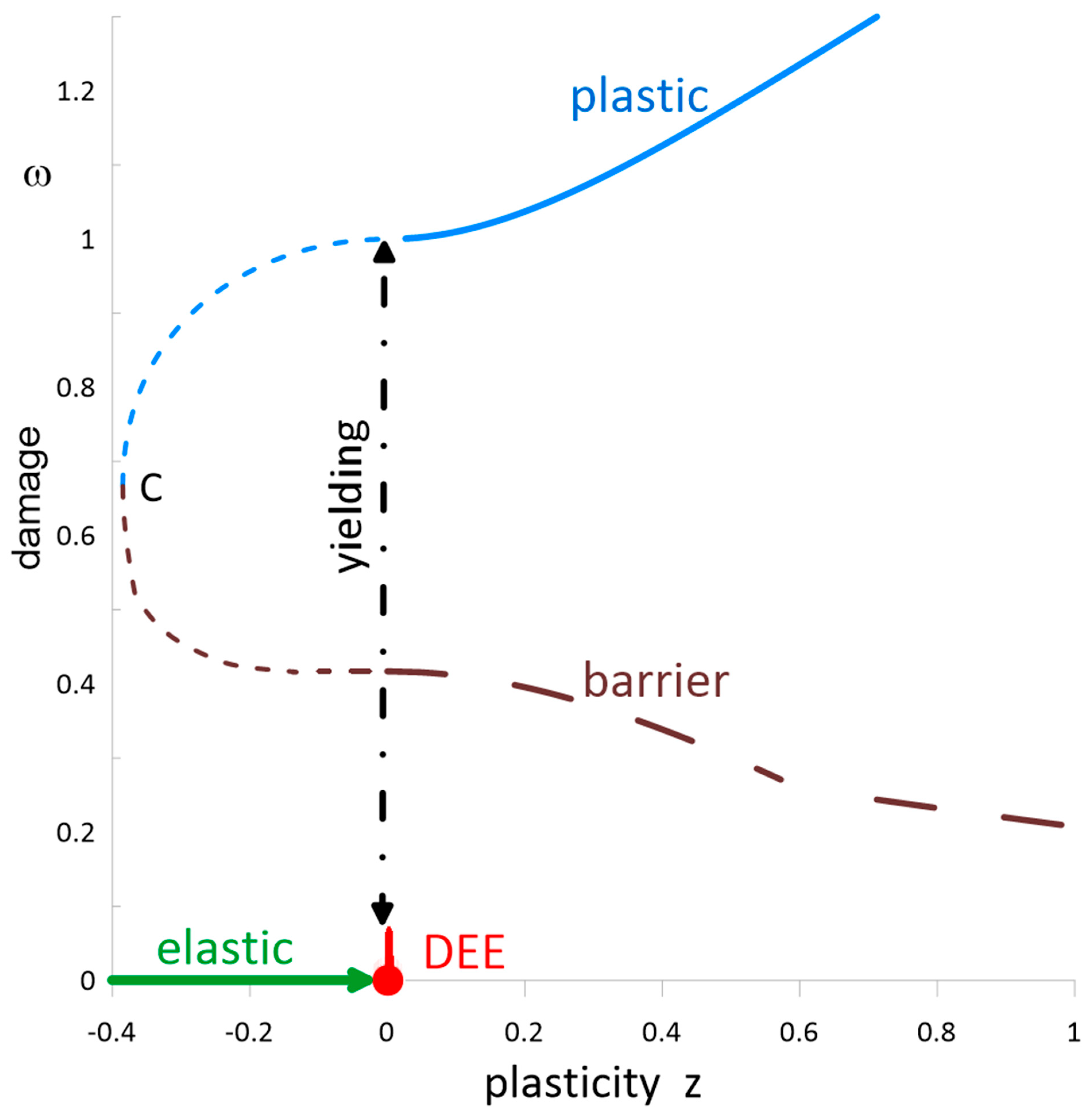
2.1. Bifurcation Theory of Plasticity

In [18], the author developed a thermodynamically consistent theory of plasticity, the main points of which are the following. (1) The state of uniaxial tension or compression of a homogeneously (uniformly) deformed virgin specimen may be described by the Helmholtz free-energy density, $f$, as a function of the total strain, $\epsilon$, and damage parameter, $\omega$, where f is a sum of the elastic, $fe$, and plastic, $fp$, contributions. (2) Initiation of plasticity (or termination of elasticity), that is, yielding, is described as a bifurcation in the phase space of the total strain and damage parameter ($\epsilon$, $\omega$), so that $\omega$ = 0 corresponds to the elastic (or quasi-elastic) state of the material and $\omega$ > 0 to its equilibrium plastic state with a damaged crystalline lattice. (3) The stress/strain reversal (unloading) in the plastic state is described as a turning point, where the material returns to the quasi-elastic state with ω = 0 (or nearly zero), and two parameters of the deformation reflecting the history of loading, called back and residual strains (ε^b, ε^r), change their values. (4) The failure of the specimen is characterized by the accumulation of certain damage values, ${\omega }^f$.

The state of uniaxial tension or compression of a deformed specimen after several stages of loading, unloading, and reloading is described by the Helmholtz free-energy density:

$$f\left(\epsilon ,{\epsilon }^r,{\epsilon }^b,\omega ,T\right)=f^e\left(\epsilon -{\epsilon }^r,T\right)+f^p\left(\omega ,\phi \right)$$

(1)

The elastic free energy, f^e, is a function of temperature, T, and the difference (ε − ε^r) of total and residual strains, where according to the shakedown theorem, the latter is the accumulation of plastic strains. In the present model, we consider only materials with linear (Hookean) elasticity: $f^e={\displaystyle \frac{1}{2}}\mu {\left(\epsilon -{\epsilon }^r\right)}^2$, where μ > 0 is the shear modulus. Then, the strain partitioning requires the residual strain to be:

$$⟦{\epsilon }^r⟧={\epsilon }_t-{\displaystyle \frac{{\sigma }_t}{\mu }}$$

(2)

where $\left({\sigma }_t,{\epsilon }_t\right)$ are the stress and strain at the turning point, and the double bracket designates a jump of the quantity at this point.

The plastic free energy, f^p, is a function of the damage parameter, ω, and loading function:

$$\phi =\phi \left(\left|\epsilon -{\epsilon }^b\right|,{\epsilon }_y;T\right)$$

(3)

which depends on the temperature, T; the difference (ε − ε^b) of the total and back strains, where the latter is related to the hardening properties of the material; and yield strain, ${\epsilon }_y\ge 0$, which may be zero. In the theory, the hardening rule is used, according to which, after unloading, the representative point of the specimen finds itself on the yield surface. Then:

$${\epsilon }^b={\epsilon }_t+{\epsilon }_y\mathrm{sign}{\displaystyle \frac{\partial \phi }{\partial \epsilon }}$$

(4)

At the turning point, the free energy experiences a drop in the amount of plastic work, even if the deformation proceeds quasi-statically:

$$⟦f⟧=-W_t^p<0$$

(5)

A more detailed description of the rate-independent plasticity may be developed based on the Preisach model of hysteresis [21].

The quasistatic processes of the loading of a virgin specimen and its subsequent unloading are shown in Figure 1. Material yielding represents a bifurcation, which is continuous by the free energy but may be continuous or discontinuous by the damage. The unloading, a turning point of loading, is characterized by the discontinuous drops of damage and free energy while the strain and stress remain continuous. In the case of discontinuous-by-damage yielding, the damage gap may be overcome by fluctuations.

2.2. Dislocation-Mediated Plasticity

If the plasticity of a specimen is mediated by the motion of dislocations, the damage parameter represents a measure of mobile dislocations. As is known [10,11,13], a 3D network, Γ, of mobile dislocation can be described by the density of its lines:

$$\rho \equiv {\displaystyle \frac{{\sum }_{\mathsf{\Gamma }}L}{V}}$$

(6)

where ${\sum }_{\mathsf{\Gamma }}L$ is the total length of its lines and V is the volume of the specimen. The entire body of the dislocation theory motivates the introduction of a damage parameter in the form of:

$$\omega \equiv b\sqrt{\rho }$$

(7)

where b is the magnitude of the Burgers vector [19]. Then, using this definition of the damage parameter, the plastic free-energy density can be described by the following expression:

$$f^p=u^p-T{s}^p=\mu {\omega }^2\left(\phi +\ln {\displaystyle \frac{1}{\omega }}+{\displaystyle \frac{\omega }{{\omega }_{*}}}\right)$$

(8)

where

$${\omega }_{*}\equiv {\displaystyle \frac{\mu }{T\psi }}$$

(9)

is a typical scale of damage in the specimen and ψ is an entropy factor, which may depend on the temperature. The damage parameter, ω, in Equations (7) and (8) accounts for the incipient and mobile dislocations, while the immobile (forest) dislocations—geometrically necessary and statistically stored—are accounted for, respectively, by the residual ε^r, Equations (1) and (2), and back ε^b, Equations (3) and (4), strains. In other words, the unloading process immobilizes the mobile dislocations and makes them a part of the elastic continuum. The discontinuous reduction in the damage parameter to zero (or nearly zero) at the turning point describes the absorption of the dislocations by the elastic continuum, not the healing of the material. The back strain in Equation (4) is determined by the forest (stored) dislocations and expresses forest hardening, while the residual strain in Equation (2) is a measure of plastic deformation determined by the geometrically necessary dislocations. Notice that although the total strain is not a state variable, that is, it depends on the deformation path, the differences of the total and residual (ε − ε^r) and the total and back (ε − ε^b) strains are the state variables, that is, they do not depend on the deformation path. In the dislocation theory, the difference (ε − ε^b) is analogous to polarization.

The damage parameter of an equilibrium state is determined by ${{\partial }_{\omega }f}^p=0$. For the elastic state, ${\omega }_e=0$. The damage parameter of the equilibrium plastic state must be found from:

$$\phi -{\displaystyle \frac{1}{2}}+\ln {\displaystyle \frac{1}{{\omega }_p}}+{\displaystyle \frac{3{\omega }_p}{2{\omega }_{*}}}=0$$

(10)

Another solution of this equation is a barrier state with ${\omega }_e<{\omega }_b<{\omega }_p$.

The dislocation-mediated plasticity described by free energy (8) is an example of discontinuous-by-damage yielding, that is, activated plasticity, which has the following distinct features. First, at the yield point, there is a jump of the damage parameter of magnitude ${\omega }_{*}$. Second, the elastic–plastic yielding has a small free-energy barrier separating the elastic and plastic states:

$${\omega }_b^y=0.417{\omega }_{*}$$

(11a)

$$f_b^p=0.0507\mu {\omega }_{*}^2$$

(11b)

which can be expressed as a barrier per unit dislocation length, that is, the Peierls stress:

$$W_P\equiv {\displaystyle \frac{F^p\left(\rho \right)}{b^2{\sum }_{\mathsf{\Gamma }}L}}={\displaystyle \frac{f_b^p}{{\left({\omega }_b^y\right)}^2}}=0.292\mu$$

(11c)

Third, there is a domain of coexistence of the elastic and plastic states with the domain of stability of the elastic state $\left[0,\right.\left.{\omega }^b\right)$ shrinking with the decrease in the loading function, φ.

In Equation (8), the dependence of the plastic free energy on strain and temperature is set by the loading function $\phi \left(\left|\epsilon -{\epsilon }^b\right|,{\epsilon }_y;T\right)$, which can be derived from a microscopic model of the dislocation network, where the strain is represented by network polarization. If bottom-up derivation is not an option, there is a top-down way to find the function $\phi \left(\left|\epsilon -{\epsilon }^b\right|,{\epsilon }_y;T\right)$ based on the analysis of the quasistatic stress–strain curve of the specimen. First, we present the flow stress as follows:

$$\sigma \left(\epsilon ,\omega \right)\equiv {\displaystyle \frac{\partial f}{\partial \epsilon }}=\mu \epsilon +\mu {\omega }^2{\displaystyle \frac{\partial \phi }{\partial \epsilon }}$$

(12)

Then, using the equilibrium presented in Equation (12), we obtain:

$$\sigma \left(\epsilon ,{\omega }_p\right)=\mu \epsilon +\mu {\omega }_p\left(1-{\displaystyle \frac{3{\omega }_p}{2{\omega }_{*}}}\right){\displaystyle \frac{\partial {\omega }_p}{\partial \epsilon }}$$

(13)

If stress is set as a function of strain, variables of this equation separate, and it is readily integrable. If stress is a function of the damage parameter also, Equation (13) can be integrated numerically. In both cases, Equation (10) and the solution of Equation (13) provide a parametric expression for $\phi \left(\left|\epsilon -{\epsilon }^b\right|,{\epsilon }_y;T\right)$. Furthermore, using the partitioning of the total strain into elastic and plastic, one can find an expression for the latter as follows:

$${\epsilon }^p=-{\omega }^2{\displaystyle \frac{\partial \phi }{\partial \epsilon }}$$

(14)

A popular model of plasticity for many metals and alloys, called ideal or perfect, describes a quasistatic, homogeneous, monotonic, and uniaxial deformation by the following stress–strain relation:

$$\sigma \left(\epsilon \right)=\left\{\begin{array}{c}\mu \epsilon ,\left|\epsilon -{\epsilon }^b\right|<{\epsilon }_y\\ \mu {\epsilon }_y,\left|\epsilon -{\epsilon }^b\right|\ge {\epsilon }_y\end{array}\right.$$

(15)

This allows one to resolve Equations (10) and (12) as follows:

$${\displaystyle \frac{\partial \phi }{\partial \epsilon }}=-{\displaystyle \frac{z}{{\omega }_p^2}}\mathrm{sign}\left(\epsilon -{\epsilon }^b\right)$$

(16a)

$${\omega }_p^2\left({\displaystyle \frac{{\omega }_p}{{\omega }_{*}}}-1\right)=z^2$$

(16b)

where a measure of the deviation beyond the yield surface, called plasticity, is introduced:

$$z\equiv \left|\epsilon -{\epsilon }^b\right|-{\epsilon }_y$$

(16c)

Notice from Equations (2), (4), and (16a) that for the quasistatic ideal deformation, ${\epsilon }^r={\epsilon }^b$. In Figure 2, the equilibrium state diagram of an ideal plastic specimen with free-energy density (8) is expressed in the phase space (z, ω).

2.3. Gradient Plasticity

As is known, deformation is fundamentally a localized process. The structural examples of this are persistent slip bands and dislocation walls, which appear both in compression and tension experiments. To describe the localization effects of inhomogeneous deformation, the author developed a theory [20] where the total free energy of a specimen is integral over the entire volume:

$$F=\int \widehat{f}{dx}^3$$

(17a)

of the free-energy density:

$$\widehat{f}=f^e+f^p+f^g$$

(17b)

where the inhomogeneous contribution is a quadratic form of the spatial gradients of the strain and damage parameter:

$$f^g={\displaystyle \frac{1}{2}}{\kappa }_{\epsilon }{\left[\mathsf{\nabla }\left(\epsilon -{\epsilon }^r\right)\right]}^2+{\displaystyle \frac{1}{2}}{\kappa }_{\omega }{\left(\mathsf{\nabla }\omega \right)}^2.$$

(17c)

Then, the stress state of the specimen is presented as the functional derivative of the free energy:

$$\sigma \left(\epsilon ,\omega \right)\equiv {\displaystyle \frac{\delta F}{\delta \epsilon }}=\mu \left(\epsilon -{\epsilon }^r\right)-{\kappa }_{\epsilon }{\nabla }^2\left(\epsilon -{\epsilon }^r\right)+\mu {\omega }^2{\displaystyle \frac{\partial \phi }{\partial \epsilon }}$$

(18)

Notice that the elastic strain (the first two terms in the r.h.s.) has an inhomogeneous contribution, which is also a function of the difference of the total and residual strains, while the plastic strain (the last term in the r.h.s.) does not have additional contributions.

If the deformed state of a specimen is set by external loading conditions, its equilibrium state must obey the Euler–Lagrange equation:

$${\displaystyle \frac{\delta F}{\delta \omega }}\equiv {\partial }_{\omega }{f}^p-{\kappa }_{\omega }{\nabla }^2\omega =0$$

(19)

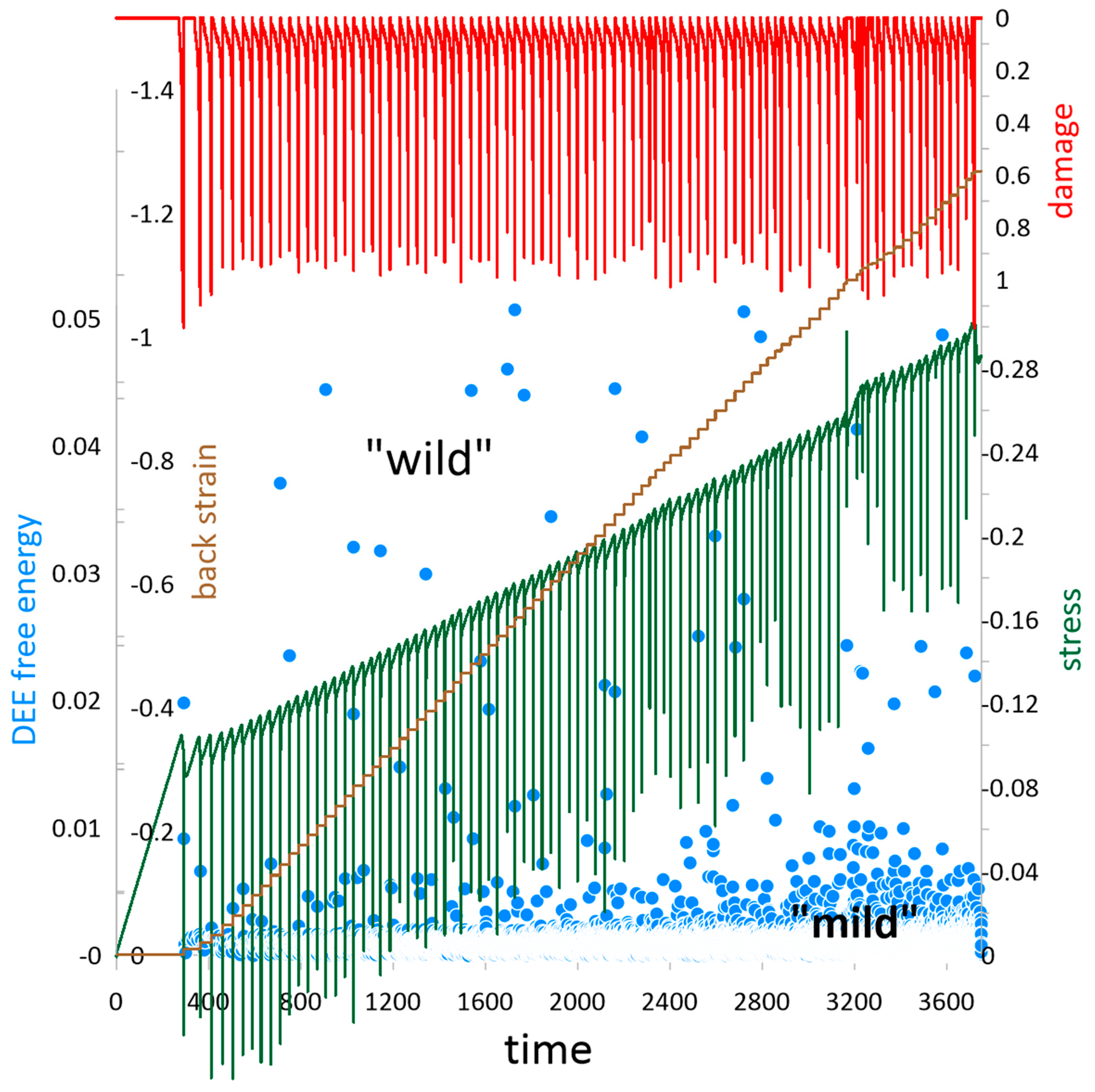
2.4. Dynamics of Damage

For the evolution of damage in a homogeneously deformed specimen in [19], the gradient-flow equation was derived:

$${\displaystyle \frac{d\omega }{dt}}=-\gamma {\displaystyle \frac{\partial f^p}{\partial \omega }}$$

(20)

where γ is the damage-parameter relaxation coefficient. Evolution of damage in an inhomogeneously deformed specimen, instead of Equation (20), obeys the inhomogeneous gradient-flow equation:

$${\displaystyle \frac{d\omega }{dt}}=-\gamma {\displaystyle \frac{\delta F}{\delta \omega }}$$

(21)

The analysis of this equation conducted in [20] shows that it allows for the heterogeneous yielding state, where the domains of undamaged elastic and damaged plastic states coexist at the yielding strain and stress. However, if the strain (stress) goes beyond the yield surface, the dislocation domain wall starts moving such that the undamaged state is replaced by the damaged one. Dimensional analysis of Equations (17c) and (21) for plastic free energy, Equation (8), shows that the speed of the wall’s motion is

$$v=\gamma \sqrt{\mu {\kappa }_{\omega }}\vartheta \left(\phi \right)$$

(22a)

where $\vartheta \left(\phi \right)$ is a dimensional function of loading. For the case of ideal plasticity, see Equation (16), the speed of motion was calculated as

$$v\approx 1.31\gamma \sqrt{\mu {\kappa }_{\omega }}{\left({\displaystyle \frac{z}{{\omega }_{*}}}\right)}^2$$

(22b)

3. Time Evolution of Deformation

In this publication, we model the compression of a specimen subjected to external loading in the strain-controlled regime with the rate of loading, which may be slow, that is, the process of compressive creep, or fast, that is, the process of shock compression. The model takes into account the following processes.

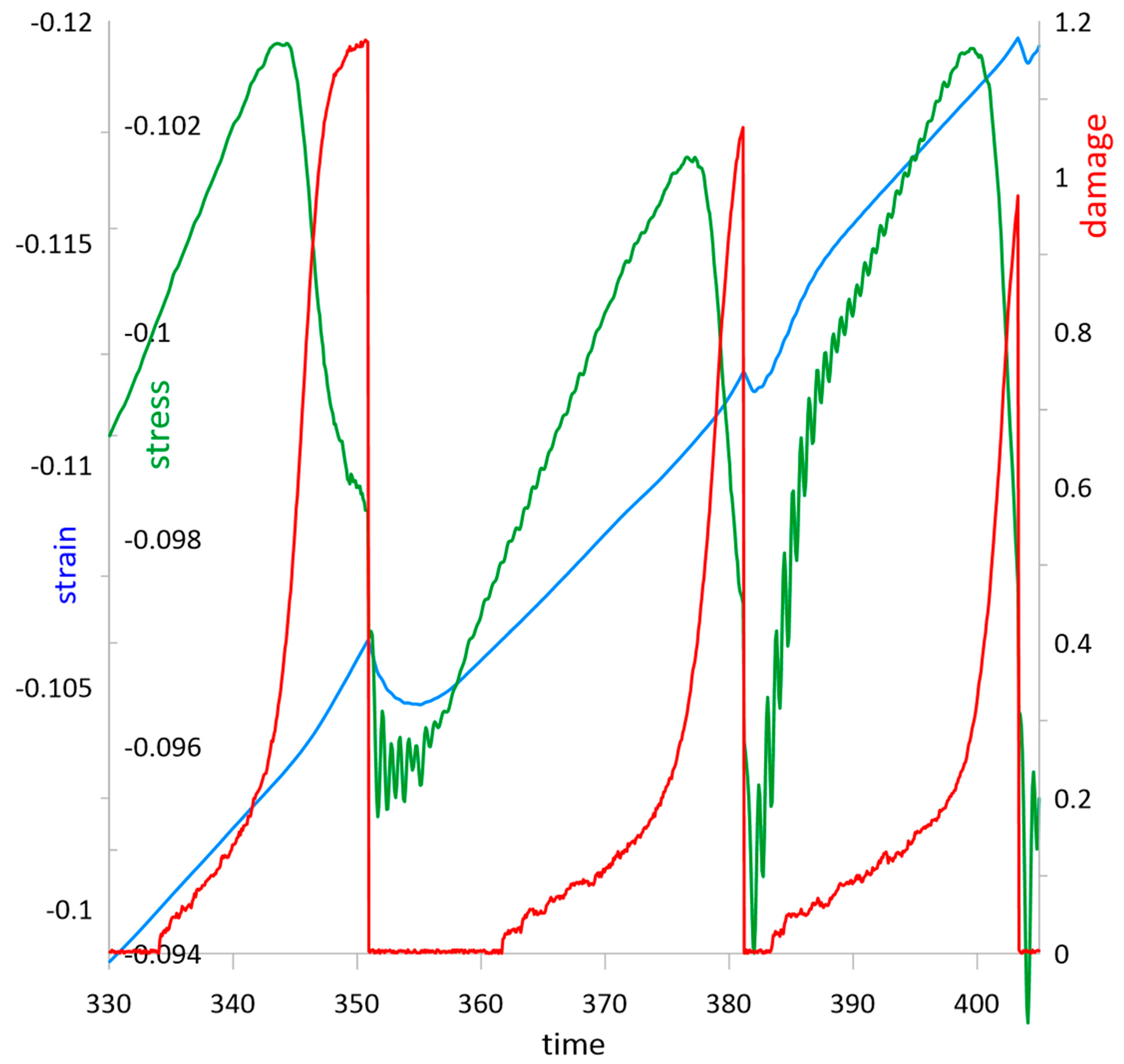
3.1. Evolution of Strain

Dynamic variations in stress and strain in the medium are described by the wave equation:

$$\varrho {\partial }_t^2{u}_i={\partial }_{x_j}{\mathsf{\Sigma }}_{ij}$$

(23)

where u_i is the displacement vector, $\varrho$ is the mass density of the medium, and ∑_ij is the total stress state of the specimen. The latter is a sum of the elasto-plastic (‘dry’) stress presented by Equation (18), dissipative (‘viscous’) stress, and the stress due to volumetric body forces, e.g., gravity, if those are significant. For the dissipative stress in the elastic domain, Landau and Lifshitz [22] derive an expression, ${\sigma }_{ij}^{\prime }=2\eta \left({\dot{\epsilon }}_{ij}-{\displaystyle \frac{1}{3}}{\dot{\epsilon }}_{kk}{\delta }_{ij}\right)+\xi {\dot{\epsilon }}_{kk}{\delta }_{ij}$, where ${\dot{\epsilon }}_{ij}$ is the rate of change in the total strain and η, ξ are the viscosity coefficients. This expression is adopted here in the elastic and plastic domains. Then, for the cases of uniaxial deformation and disregarding gravity, we obtain:

$$\mathsf{\Sigma }=\sigma \left(\epsilon ,\omega \right)+\eta {\displaystyle \frac{d\epsilon }{dt}}$$

(24)

For the uniaxial deformation of a long, thin rod differentiating Equation (23) with respect to the spatial coordinate, we obtain the generalized wave equation for the strain field:

$$\varrho {\partial }_t^2\epsilon ={\partial }_x^2\mathsf{\Sigma }$$

(25)

3.2. Evolution of Damage

Evolution of damage is described by Equation (21). As the gradient ${\partial }_{\omega }{f}^p$ changes sign at the barrier state, the domain of the damage parameter evolution ${\omega }_e<{\omega }_p$ breaks down into two subdomains, ${\omega }_e<{\omega }_b$ and ${\omega }_b<{\omega }_p$, such that the damage is driven to decrease in the former and increase in the latter. For the domain of damage increase, one can define the characteristic time as follows

$${\mathsf{{\rm T}}}_p\equiv {\displaystyle \frac{{\omega }_p-{\omega }_b}{\underset{t}{\max }\left|{\partial }_t\omega \right|}}={\displaystyle \frac{1}{\gamma \mu }}{\displaystyle \frac{{\omega }_p-{\omega }_b}{{\omega }_m\left(3\frac{{\omega }_m}{{\omega }_{*}}-2\right)}}\approx {\displaystyle \frac{4.43}{\gamma \mu }}$$

(26a)

where ${\omega }_m$ is the solution to the following equation:

$$\phi -{\displaystyle \frac{3}{2}}+\ln {\displaystyle \frac{1}{{\omega }_m}}+3{\displaystyle \frac{{\omega }_m}{{\omega }_{*}}}=0$$

(26b)

For the domain of damage decrease, the characteristic time is $T_e\approx 2.17/\gamma \mu$.

The spatial gradients of Equation (21) do not change the breakdown of the domain ${\omega }_e<{\omega }_p$ into the subdomain of damage increase and decrease. Hence, the evolution of damage cannot be described by the homogeneous gradient-flow equation alone. The subdomain ${\omega }_e<{\omega }_b$ must be traversed by fluctuations in damage also.

Let us assume that under conditions of thermodynamic equilibrium, the elastic state contains a fluctuating network of dislocations described by the average density ${\rho }_n>0$, damage parameter ${\omega }_n=b\sqrt{{\rho }_n}$, and variance ${\omega }_n^2/3$. The fluctuations are caused by the operation of various sources of dislocation nucleation and annihilation, where nucleation prevails. The value ${\omega }_n$ is much smaller than the equilibrium value of the damage parameter in the plastic state, ${\omega }_{*}$, and may depend on the temperature and state of strain. In this publication, we assume that ${\omega }_n\approx 3\times {10}^{-3}{\omega }_{*}$; the sources of fluctuations in the specimen are considered elsewhere.

The evolution of such a network may be described by the following Langevin-type equation:

$${\displaystyle \frac{d\omega }{dt}}=-\gamma {\displaystyle \frac{\delta F}{\delta \omega }}+\varpi \left(\mathit{x},t\right)$$

(27)

where the Langevin force (noise) $\varpi \left(\mathit{x},t\right)$ has the following correlation properties:

$$〈\varpi \left(\mathit{x},t\right)〉=\gamma {\omega }_n{{\partial }_{\omega }^{2}f}^p\left({\omega }_n,\phi \right)$$

(28a)

$$〈\varpi \left({\mathit{x}}_1,t_1\right)\varpi \left({\mathit{x}}_2,t_2\right)〉={\displaystyle \frac{8}{3}}\gamma \mathsf{\Omega }{\omega }_n^2{{\partial }_{\omega }^{2}f}^p\left({\omega }_n,\phi \right)\delta \left({\mathit{x}}_2-{\mathit{x}}_1\right)\delta \left(t_2-t_1\right)$$

(28b)

where the angle brackets represent statistical averaging; Ω = r^d is the representative volume of the fluctuation correlations whose characteristic radius and time are:

$$r=\sqrt{{\displaystyle \frac{{\kappa }_{\omega }}{{{\partial }_{\omega }^{2}f}^p\left({\omega }_n,\phi \right)}}}$$

(29a)

$$\tau ={\left[\gamma {{\partial }_{\omega }^{2}f}^p\left({\omega }_n,\phi \right)\right]}^{-1}$$

(29b)

and d is the dimensionality of the specimen. Such a Langevin force can be reproduced by the following additive-noise function:

$$\varpi \left(x,t\right)=2\gamma {\omega }_n{{\partial }_{\omega }^{2}f}^p\left({\omega }_n,\phi \right)\xi \left(\Delta x,\Delta t;d\right)$$

(30)

where ξ is a random variable uniformly distributed on the interval $\left[0,1\right]$; Δx and Δt are the representative size and time inside which the noise, ξ, is strongly correlated. For the correlation function of the Langevin force expressed by Equation (30) to be equal to expression (28b), Δx and Δt must be equal to the correlation radius, Equation (29a), and time, Equation (29b), where the derivatives of the free energy, Equation (8), may be taken at the point of yielding:

$${\partial }_{\omega }{f}^p\left({\omega }_n,{\phi }_y\right)=\mu {\omega }_n\left[2\ln {\displaystyle \frac{{\omega }_{*}}{{\omega }_n}}+3\left({\displaystyle \frac{{\omega }_n}{{\omega }_{*}}}-1\right)\right]\approx 2\mu {\omega }_n\ln {\displaystyle \frac{{\omega }_{*}}{{\omega }_n}}$$

(31a)

$${\partial }_{\omega }^2{f}^p\left({\omega }_n,{\phi }_y\right)=2\mu \left(\ln {\displaystyle \frac{{\omega }_{*}}{{\omega }_n}}+3{\displaystyle \frac{{\omega }_n}{{\omega }_{*}}}-{\displaystyle \frac{5}{2}}\right)\approx 2\mu \ln {\displaystyle \frac{{\omega }_{*}}{{\omega }_n}}$$

(31b)

Then, the characteristic time of fluctuational growth may be estimated as follows:

$${\mathsf{{\rm T}}}_n\equiv {\displaystyle \frac{{\omega }_b}{〈\varpi \left(\mathit{x},t\right)〉}}\approx {\displaystyle \frac{1}{\gamma \mu }}{\displaystyle \frac{{\omega }_b}{2{\omega }_n\ln \frac{{\omega }_{*}}{{\omega }_n}}}$$

(32)

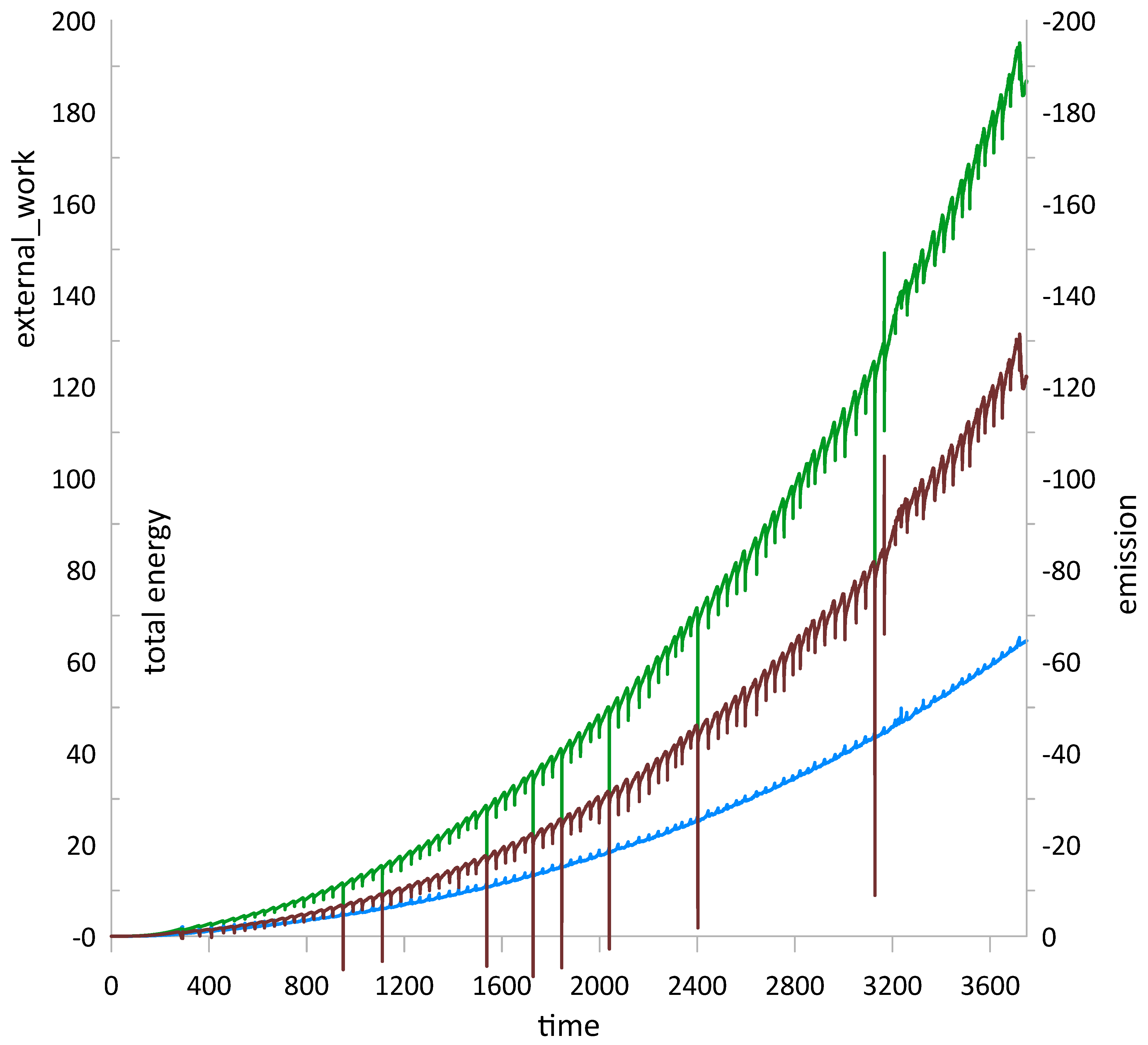
3.3. Free-Energy Balance

First, notice that the Langevin force, Equation (30), has a nonvanishing correlation with the driving force, Equation (19). Indeed:

$$\langle {\displaystyle \frac{\delta F}{\delta \omega }}\left({\mathit{x}}_1,t_1\right)\varpi \left({\mathit{x}}_2,t_2\right)\rangle =\gamma {\omega }_n{{\partial }_{\omega }f}^p\left({\omega }_n,{\phi }_y\right){{\partial }_{\omega }^{2}f}^p\left({\omega }_n,{\phi }_y\right)\approx 4\gamma {\left(\mu {\omega }_n\ln {\displaystyle \frac{{\omega }_{*}}{{\omega }_n}}\right)}^2$$

(33)

Then, the free-energy balance in the representative volume during the representative time of the fluctuations is:

$$\begin{array}{c}∆F={\int }_{\tau }\delta F={\int }_{\tau }{\int }_{\mathsf{\Omega }}d{x}^3\left\{{\displaystyle \frac{\delta F}{\delta \epsilon }}\delta \epsilon +{\displaystyle \frac{\delta F}{\delta \omega }}\delta \omega \right\}=\tau {\int }_{\mathsf{\Omega }}d{x}^3\left\{\langle \sigma {\displaystyle \frac{d\epsilon }{dt}}\rangle +\langle {\displaystyle \frac{\delta F}{\delta \omega }}{\displaystyle \frac{d\omega }{dt}}\rangle \right\}\\ =\tau \mathsf{\Omega }\left\{\left[{\displaystyle \frac{1}{\eta }}〈\sigma \mathsf{\Sigma }〉+\langle {\displaystyle \frac{\delta F}{\delta \omega }}\varpi \rangle \right]-\left[{\displaystyle \frac{1}{\eta }}〈{\sigma }^2〉+\gamma \langle {\left({\displaystyle \frac{\delta F}{\delta \omega }}\right)}^2\rangle \right]\right\}\end{array}$$

(34)

where the time integration is replaced with averaging using the ergodic properties of the process of dislocation nucleation and annihilation. The first bracket in this expression contains contributions due to the mechanical work of the external load and microscopic work of the dislocation sources, which lead to an increase in free energy. The second bracket contains strictly dissipative contributions due to viscosity and stress relaxation processes.

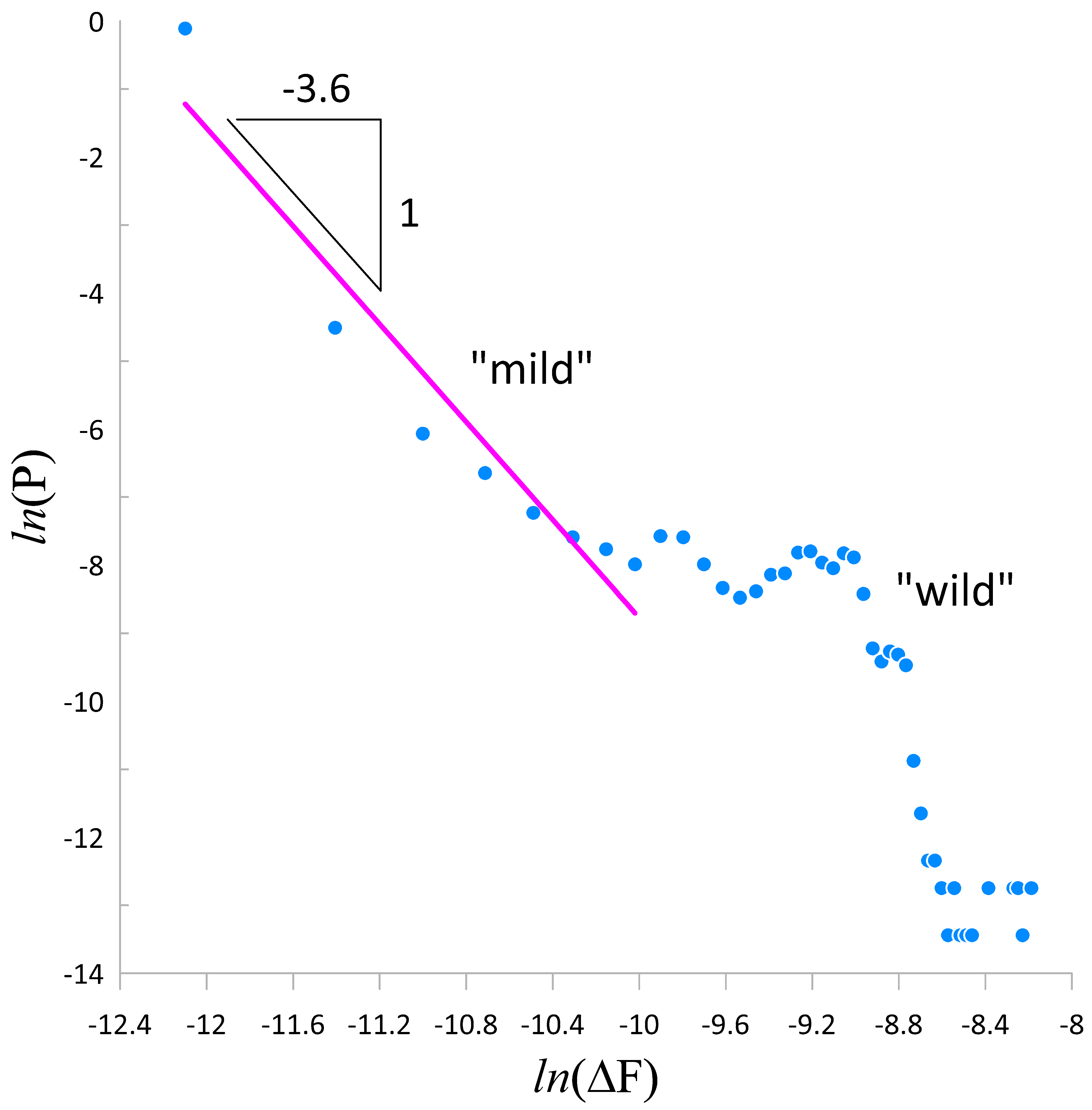
3.4. Dislocation Emission Event

As stated in Section 2.2, the evolution of a dislocation network constitutes plastic deformation, which is described in the theory as the increase in the damage parameter ω. The stress/strain reversal in the plastic state of a representative volume of a specimen is a turning point in the phase space of the material, where it returns to the quasi-elastic state with <ω> = ω_n, and two parameters of the deformation, namely back and residual strains (ε^b, ε^r), change their values. This is the dislocation emission event (DEE), which comprises the sudden breaking of the network’s evolution. It is triggered by local unloading, which may be caused by external conditions or is random, that is, due to local fluctuations. The unloading process immobilizes the mobile dislocations and makes them a part of the elastic continuum of the material. In the theory, they emerge in the form of updated back and residual strains (ε^b, ε^r), with the former describing forest hardening by statistically stored dislocations and the latter, plastic strain, due to geometrically necessary dislocations. The size of the representative volume of the DEE is the correlation radius, Equation (29a), and the duration of the event is the correlation time, Equation (29b). Together with the damage drop, the free energy of the representative volume also drops during the event. The energy drop may appear in the form of dissipation by the processes described by Equations (24) and (27). However, due to the slowness of these processes, it is most likely to appear in the form of an acoustic emission described by Equations (23) and (25). According to the theory, in quasistatic unloading (stress/strain reversal), stress must remain continuous, see Figure 1. However, a drop in stress may appear as a result of dynamic processes described by Equations (24), (25), and (27). Notice that the DEE describes the absorption of dislocations by the elastic continuum, not the healing of the material.

3.5. Initial and Boundary Conditions

Initially, the undeformed rod of length L₀ is in the elastic state:

$$t=0:\epsilon ={\epsilon }^b={\epsilon }^r=0;〈\omega \left(x,0\right)〉={\omega }_n$$

(35)

In the process of deformation, one end of the rod is held fixed at all times:

$$x=0:\epsilon ={\epsilon }^b={\epsilon }^r=0;〈\omega \left(0,t\right)〉={\omega }_n$$

(36a)

while the other end is loaded in the strain-control regime:

$$x=L_0:\epsilon =\dot{\epsilon }t;{\partial }_x\omega =0$$

(36b)

where $\dot{\epsilon }$ is the strain rate. As the loading proceeds, the length of the rod changes:

$$L=L_0+{\int }_0^{L_0}\epsilon dx.$$

(37)

3.6. Scaling and Dimensionless Properties

The free energy (8) motivates the following scaling of strain, damage, stress, and energy density:

$$\left[\epsilon \right]=\left[\omega \right]={\omega }_{*};\left[\sigma \right]=\mu {\omega }_{*};\left[f\right]=\mu {\omega }_{*}^2$$

(38)

while the dynamic Equation (27) and correlation properties of the noise (28) motivate the following scaling of space, time, and noise:

$$\left[x\right]=\sqrt{{\displaystyle \frac{{\kappa }_{\omega }}{\mu }}};\left[t\right]={\displaystyle \frac{1}{\gamma \mu }};\left[\varpi \right]=\gamma \mu {\omega }_{*}$$

(39)

Then, the scaled Equations (18), (24), (25), (27), (30), and (31b) take the form:

$${\partial }_t\omega ={\partial }_x^2\omega -{\partial }_{\omega }{f}^p\left(\omega ,\phi \right)+\varpi \left(x,t\right)$$

(40a)

$$\varpi \left(x,t\right)\approx 4{\omega }_n\ln {\displaystyle \frac{1}{{\omega }_n}}\xi \left(\Delta x,\Delta t\right)$$

(40b)

and

$${\partial }_t^2\epsilon =G{\partial }_x^2\mathsf{\Sigma }$$

(41a)

$$\mathsf{\Sigma }=\left(\epsilon -{\epsilon }^r\right)-k{\partial }_x^2\left(\epsilon -{\epsilon }^r\right)+{\omega }^2{\partial }_{\epsilon }\phi +u{\partial }_t\epsilon$$

(41b)

where the following dimensionless properties of the material arise:

$$G={\left({\displaystyle \frac{c\left[t\right]}{\left[x\right]}}\right)}^2={\displaystyle \frac{c^2}{{\gamma }^2\mu {\kappa }_{\omega }}}={\left(\varrho {\kappa }_{\omega }{\gamma }^2\right)}^{-1}$$

(42a)

is the ratio of the squares of the speeds of sound and dislocation domain wall,

$$k={\displaystyle \frac{{\kappa }_{\epsilon }}{{\kappa }_{\omega }}}$$

(42b)

is the ratio of the gradient coefficients,

$$u=\gamma \eta$$

(42c)

is the ratio of the dissipative coefficients, and

$$c=\sqrt{{\displaystyle \frac{\mu }{\varrho }}}$$

(42d)

is the speed of sound in the rod.

Table 1. Mechanical and dimensionless properties of a typical metal, e.g., copper.

Property	Designation	Unit	Experimental Quantity
Shear modulus	μ	Pa	5 × 1010
Mass density	$\varrho$	kg/m3	5 × 104
Speed of sound	c	m/s	103
0.2%-yield strength	${\widehat{\sigma }}_y$	Pa	108
Yielding	${\epsilon }_y$		2 × 10−3
Ductility	${\widehat{\epsilon }}_f$		0.5
Burgers vector	b	m	10−10
Dislocation density scale of plastic state	${\rho }_{*}$	1/m2	1014
Dislocation density scale of elastic state	${\rho }_n$	1/m2	109
Strain gradient coefficient	${\kappa }_{\epsilon }$	J/m	10−5
Dislocation gradient coefficient	${\kappa }_{\omega }$	J/m	10−5
Viscosity	η	Pa·s	104
Relaxation coefficient	γ	(Pa·s)−1	10−2
Damage scale	${\omega }_{*}=b\sqrt{{\rho }_{*}}$		10−3
Length scale	$\left[x\right]=\sqrt{{\kappa }_{\omega }/\mu }$	nm	14
Time scale	$\left[t\right]=1/\gamma \mu$	ns	2
Shock length scale	${\left[x\right]}_s=c/\gamma \mu$	μm	4
Creep time scale	${\left[t\right]}_c=\eta /\mu$	μs	0.2
Stress scale	$\left[\sigma \right]=\mu {\omega }_{*}$	Pa	5 × 107
Energy density scale	$\left[f\right]=\mu {\omega }_{*}^2$	J/m3	5 × 104
Noise scale	$\left[\varpi \right]=\gamma \mu {\omega }_{*}$	1/s	5 × 105
Ratio of speed scales	$G={\left(\varrho {\kappa }_{\omega }{\gamma }^2\right)}^{-1}$		2 × 104
Ratio of time scales	$u=\gamma \eta$		102
Ratio of gradient coefficients	$k={\kappa }_{\epsilon }/{\kappa }_{\omega }$		1

contains the mechanical properties and their dimensionless combinations for a typical metal-like copper. The values of the strain and damage gradient coefficients are taken as equal to 10⁻⁵ J/m. The values of the dislocation densities are estimated as ${\rho }_n\approx {10}^9 {\mathrm{m}}^{-2}$ and ${\rho }_{*}\approx {10}^{14} {\mathrm{m}}^{-2}$, which yields $r\approx 5\mathrm{nm}$ and $\tau \approx 0.25\mathrm{ns}$ for the correlation radius and time, $f_b^p\approx 2.5\times {10}^3 \mathrm{J}/{\mathrm{m}}^3$ for the Peierls barrier, and $\left[∆F\right]=\left[f\right]·r^3\approx 6.25\mathrm{zJ}$ for the energy scale of a DEE.

4. Numerical Implementation

The deformation of a specimen whose properties are characterized by the dimensionless parameters G, k, and u, Equation (42), is described by the dynamic Equations (40) and (41), with the dimensionless strain rate, $\dot{\epsilon }$; initial length, $L_0$; and duration of the process, $T_0$; as the control parameters. The local dislocation emission events (DEEs) were characterized by the decrease in the free energy in the representative volumes.

High values of G and u, see Table 1, make computations by Equation (41) technically challenging. To avoid this, we considered two limiting cases of the loading of a specimen: fast and slow. Mechanically, the former can be considered as shock compression while the latter as compressive creep. In the case of shock loading, the material viscosity may be disregarded, that is, Equation (41b) takes the form:

$$\mathsf{\Sigma }=\left(\epsilon -{\epsilon }^r\right)-k{\partial }_x^2\left(\epsilon -{\epsilon }^r\right)+{\omega }^2{\partial }_{\epsilon }\phi$$

(43)

In the case of creep loading, the inertial effects of the deformation may be disregarded, and Equation (23) shows that $\mathsf{\Sigma }=\mathrm{const}\left(x\right)$. Applying this result to the loaded end, $x=L_0$, we obtain $\mathsf{\Sigma }=\dot{\epsilon }\left(t+u\right)$, which yields the dynamic equation for the strain in the form:

$$u{\partial }_t\epsilon =k{\partial }_x^2\left(\epsilon -{\epsilon }^r\right)-\left(\epsilon -{\epsilon }^r\right)-{\omega }^2{\partial }_{\epsilon }\phi +\dot{\epsilon }\left(t+u\right)$$

(44)

Notice that Equations (40) and (44) do not allow us to model the terminal stage of creep because material failure is not included.

To speed up the computations, the dynamic Equations (40), (41), and (44) were rescaled with

$${\left[x\right]}_s=\left[x\right]\sqrt{G}={\displaystyle \frac{1}{\gamma \sqrt{\mu \varrho }}}$$

(45)

in the case of shock loading and

$${\left[t\right]}_c={\displaystyle \frac{\eta }{\mu }}$$

(46)

in the case of creep loading. The control parameters, strain rate, initial length, and duration of the process, together with the material properties, G and u, in creep and shock regimes of loading are shown in

Table 2. Control parameters: strain rate, initial length, and duration of the process, and material properties: G and u, in creep and shock regimes of loading.

	$\dot{\mathit{\epsilon }}$ (s−1)	${\mathit{L}}_0$ (μm)	${\mathit{T}}_0$ (μs)	G	u
Creep	5	1.4 × 102	5 × 103		0.001 ÷ 1
Shock	5 × 103	4 × 104	7.5	5 ÷ 20

.

Equations (40), (41), or (44) were discretized using the explicit numerical method with the correlation radius and time, Equation (29), as the discretization length Δx and time Δt. The Langevin noise in Equation (30) was represented by the random variable ξ uniformly distributed on the interval $\left[0,1\right]$. In the cases when computations were conducted using smaller time increments, the results were not averaged over the time period, Δt. For the probability density function calculations, the total range of energy drops was divided into 50 bins.

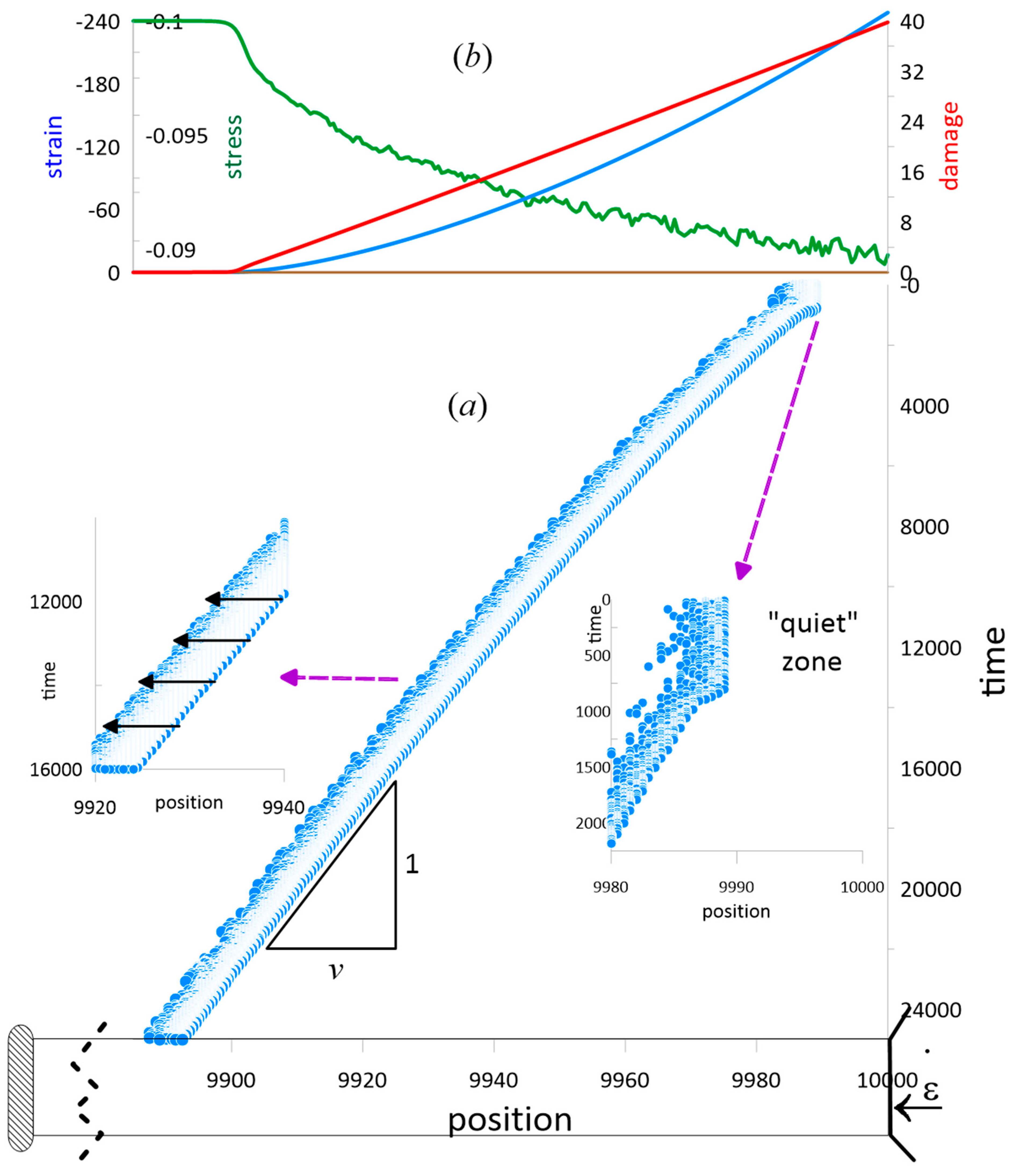
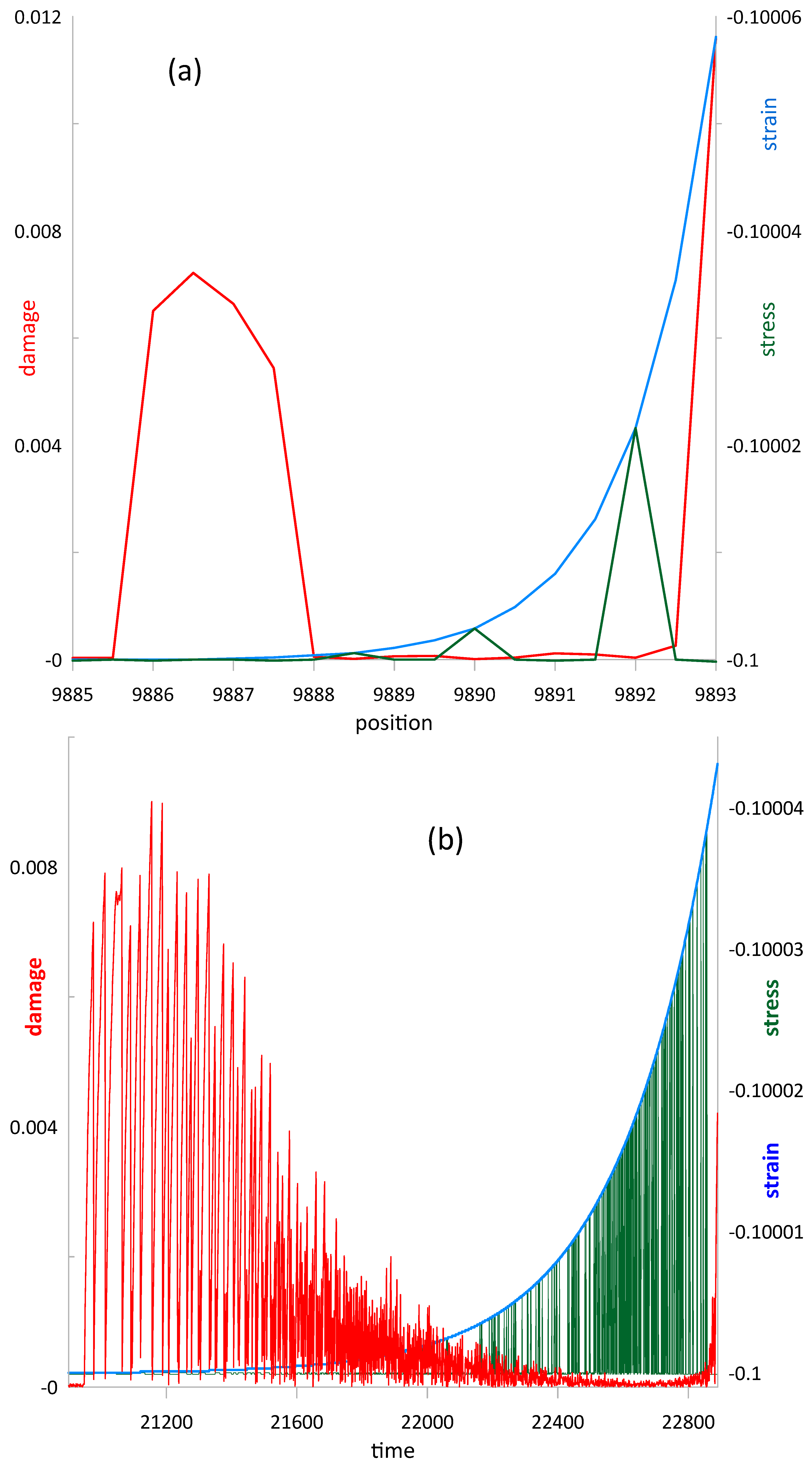
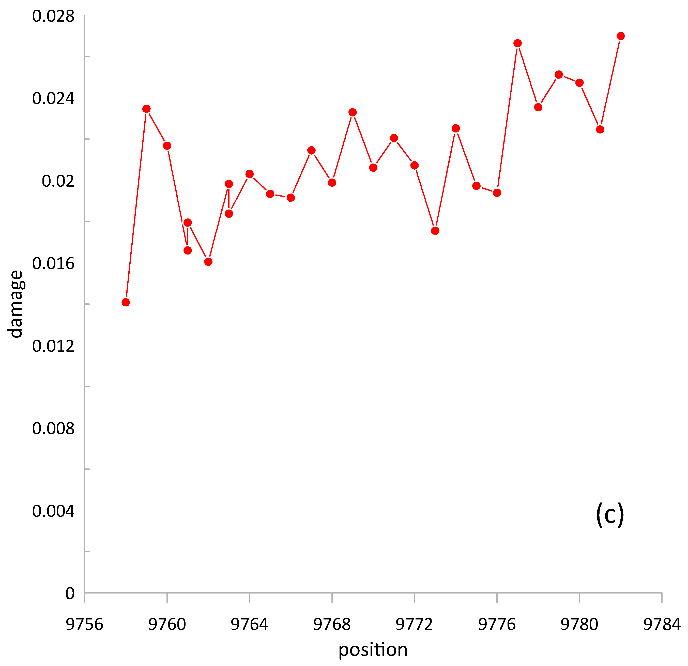
5. Compressive Creep

Figure 3 shows the time distribution of the DEEs in the rod and the compressive stress on its loaded end in the compressive creep regime of loading. After a short transient time, the DEEs settle in a stationary regime, which can be divided into ‘mild’ and ‘wild’ categories, where the latter clearly manifests the presence of two energy scales.

Figure 4 depicts the probability density function of the DEEs, which shows that the ‘mild’ part of the spectrum is scale-free, while the ‘wild; part clearly manifests two recognizable energy scales. The scale-free exponent is approximately two-times greater than the experimentally observed result.

Individual dislocation emission events self-organize into slip bands of practically a fixed length, which propagate through the specimen as a train wave, that is, at a practically constant speed leaving behind the highly strained, severely damaged, but not highly stressed, part of the specimen, see Figure 5. Near the loaded end of the specimen there is a ‘quiet zone’, which does not experience any events.

The spatial structure of a slip band, shown in Figure 6a, represents a dislocation pileup against the concentration of strain instead of the structural irregularities. Figure 6b shows the temporal variation in the strain, stress, and damage in a representative volume near the loaded end. Sharp damage drops appear because DEEs are turning points of deformation, see Figure 1. The stress drops have a dynamic nature.

The juxtaposition of Figure 6a,b clearly shows that the temporal distributions of damage and stress in DEEs are modulated forms of the spatial distributions of the same quantities. This reveals the traveling-wave nature of the process and allows one to deduce a formula for the propagating characteristics of deformation:

$$\epsilon =g\left(x-vt\right)$$

(47a)

$$\omega =f\left(t\right)g\left(x-vt\right)$$

(47b)

where $v$ is the slip band speed. In Figure 7, the speed, $v$, is shown as a function of the ratio of dissipative coefficients, u (Equation (42c)) for the fixed strain rate, $\dot{\epsilon }$, and compared with the speed of the dislocation domain wall motion, Equation (22b), which, using the scaling of Equations (38), (39), and (46), becomes: $v\approx 1.31u{z}^2$. A good match is a convincing argument that the process of slip band propagation is the motion of dislocation domains.

In the compressive creep ‘experiments’, the specimen did not harden, which is manifested by an almost constant time-averaged stress on the loaded end, see Figure 3, and practically zero back strain in the deformed part of the specimen, see Figure 5b. the lack of hardening is in accordance with the ideal plastic properties of the simulated material.

Finally, DEEs can be laid out in the phase space $\left(z,\omega \right)$ of Figure 2, which makes us conclude that the dislocation emission events take place on the yield surface of the specimen.

6. Shock Compression

Figure 8 depicts the time distribution of DEEs in the rod together with the compressive stress, back strain, and amount of damage on its loaded end in the shock compression regime of loading. Similar to the case of creep loading, sharp damage and stress drops are prominent. Compared to creep loading, see Sec. V, shock loading is characterized by the significantly greater energy of DEEs, c.f. Figure 3. In the case of impact loading, the events also break down into two categories—low emissions (‘mild’) and high emissions (‘wild’)—with the watershed value in the range of 0.005 ÷ 0.01. However, there also appears the upper level of emissions equal to the free-energy barrier separating the elastic and plastic states, see Equation (11b) and Figure 2.

The probability distribution function of DEE energies follows the log-log relationship with the exponent (−2.77), see Figure 9, which is still higher than the experimentally observed value of (−1.7). The upper-level cut-off is prominent.

Figure 10 shows the free-energy balance in the specimen, where its total energy plus the emissions is equal to the external work of loading.

Figure 11 presents the space–time map of DEEs in a shock-loaded specimen. It shows that the emission front propagates with speed close to the speed of sound and that, contrary to the case of creep loading, the events densely cover the deformed domain, leaving no quiet zones, see Figure 11a. A high-resolution observation of the first 600 time-units of the process, see Figure 11b, shows that the individual events self-organize into slip bands and avalanches. Periodic slips at the loaded end of the specimen cause stress drops while the avalanches propagate into the bulk of the specimen faster than sound. A closer analysis of Figure 11b shows that the speed of an avalanche depends on its size, with the smaller ones moving faster than the larger ones. The spatial structure of the avalanche marked by an oval in Figure 11b is shown in Figure 11c. Like the case of creep loading, see Figure 6a, it represents a dislocation pileup against the concentration of strain. The self-organization of DEEs into slip bands and avalanches is due to the plastic connectivity of the medium expressed by the damage gradient coefficient ${\kappa }_{\omega }$, while the motion of the avalanches at a supersonic speed is due to the dispersion of the medium expressed by the strain gradient coefficient ${\kappa }_{\epsilon }$ in Equation (17c).

Deformation of a shock-compressed specimen leads to significant hardening with time, see Figure 3 and Figure 8, which leaves the deformed domain slightly damaged and severely stressed beyond the yield point, see Figure 11a. Such hardening leaves permanent traces in the specimen, which becomes inhomogeneously hardened after the removal of the load. Impact hardening occurs due to the high speed of loading despite the perfectly plastic properties of the material. It is a dynamic effect of impact loading.

The high-resolution DEE map, Figure 11b, also manifests the temporal periodicity of the slip bands and avalanches. To reveal the nature of the time separation between the events, we show in Figure 12 the first three slip bands of the specimen, which present the following scenario of evolution of deformation in a representative volume leading up to a dislocation emission event. After crossing the yield surface, damage increases by the fluctuation mechanism against the thermodynamic ‘driving force’ until crossing the free-energy barrier and by the ‘driving force’ beyond the barrier, see Equation (27). The damage increase causes stress to decrease (by absolute value), see Equation (18), which leads to the next unloading, that is, the next DEE. One may lay out DEEs in the phase space $\left(z,\omega \right)$ and, like in the case of creep loading, find them on the yield surface, see Figure 2. Then, the longevity of periodicity may be analyzed based on the damage evolution in Equation (27). Indeed, adding the characteristic times of damage increase, decrease, and fluctuational growth (Equations (26) and (32)), we obtain: $P=T_p+T_e+T_n\approx 16.6\left[t\right]$, which is confirmed by Figure 12.

Finally, Figure 13 is a stress–damage–strain diagram for a representative point 100 units away from the loaded end, see Figure 11b. First, compare it to a time series of the same events in Figure 12 and notice that the strain representation smothers the instabilities of deformation. Second, compare it to Figure 1 and find the basic features of the cycle: yielding and DEE damage drops. However, contrary to its quasistatic counterpart, dynamic yielding has a fluctuational component.

7. Discussion

In this article, we simulate an inhomogeneous plastic deformation process in a relatively large specimen, 100 μm ÷ 100 mm, subjected to the strain-controlled loading of variable speed. To perform this, we use a thermodynamically consistent mean-field theory of plasticity [18,19,20], according to which the state of a deformed specimen is described by the free energy as a function of the total strain and damage parameter. One can introduce the principle of a thermodynamic alternative according to which a quasistatic thermodynamic process can be either reversible or hysteretic. Then, plastic deformation becomes an example of a hysteretic thermodynamic process, while phase transition becomes an example of a reversible one. If the plasticity of a specimen is mediated by the motion of dislocations, the damage parameter represents a measure of only mobile dislocations while the immobile dislocations—geometrically necessary and statistically stored—are a part of the elastic continuum characterized by the back and residual strains. For instance, forest (stored) dislocations determine the back strain, which describes forest hardening, while the residual strain is a measure of plastic deformation determined by the geometrically necessary dislocations.

Dynamically, the deformation of a specimen was described by the elastic wave equation, the equation of strain-rate sensitivity, and the damage-evolution Langevin-type equation with additive noise. The latter accounts for the dislocation fluctuations due to nucleation (release) and annihilation (arrest), with nucleation prevailing. In this theory, the dislocation emission event (DEE) is a turning point of plasticity in a representative volume, that is, the stress/strain reversals caused by local unloading. The latter may be caused by the overall unloading of the specimen or local fluctuations in damage. In other words, in this theory, a DEE is dislocation pinning while in traditional theories it is the depinning of the same event.

In this article, we consider uniaxial loading with the loading axis oriented along the single-slip direction in the specimen subjected to two limiting cases of loading, fast and slow, where the former can be considered as shock compression while the latter as compressive creep. Many of the simulated features of the processes were observed experimentally. DEEs were characterized by a sharp decrease in the free energy in the representative volumes. The external work of loading and total emissions from the entire specimen were also registered. The sporadic appearance of DEEs throughout the parts of the specimen strained beyond the point of yielding were observed. The events preceded by the fluctuation assisted yielding and were found to take place on the yield surface. DEEs consisted of local bursts of stress and release of energy, which stochastically appeared as small, ‘mild’ events or large, ‘wild’ events. The ‘mild’ DEEs are scale-free, have a Gaussian distribution, and do not have a strong influence over the ‘wild’ ones. The latter were not scale-free. We observed the self-organized spatial clustering of DEEs into slip bands and/or avalanches. In the strain-damage phase space, DEEs took place on the yield surface, practically independently of external loading conditions. However, simulations of the creep and shock loading revealed structural differences of the subsequent deformation. In creep compression, it may be characterized as an avalanche of slip bands, while in shock compression the slip bands and avalanches occur separately with the avalanche ‘free flight’ velocity greater than the speed of sound.

The 1D model did not include failure, aging, or material degrading in the form of changing properties, and temperature effect on deformation. These processes will be addressed in future work, where we also plan to develop a 2D/3D model to study size effect and multi-axial loading. We also plan to apply the developed method to the deformation of real, anisotropic, polycrystalline materials with a crystallographic texture.

8. Conclusions

We developed a theory and conducted simulations of the uniaxial loading of a single-slip specimen of a relatively large size: 100 μm ÷ 100 mm. The main outcomes of the theory/simulations are:

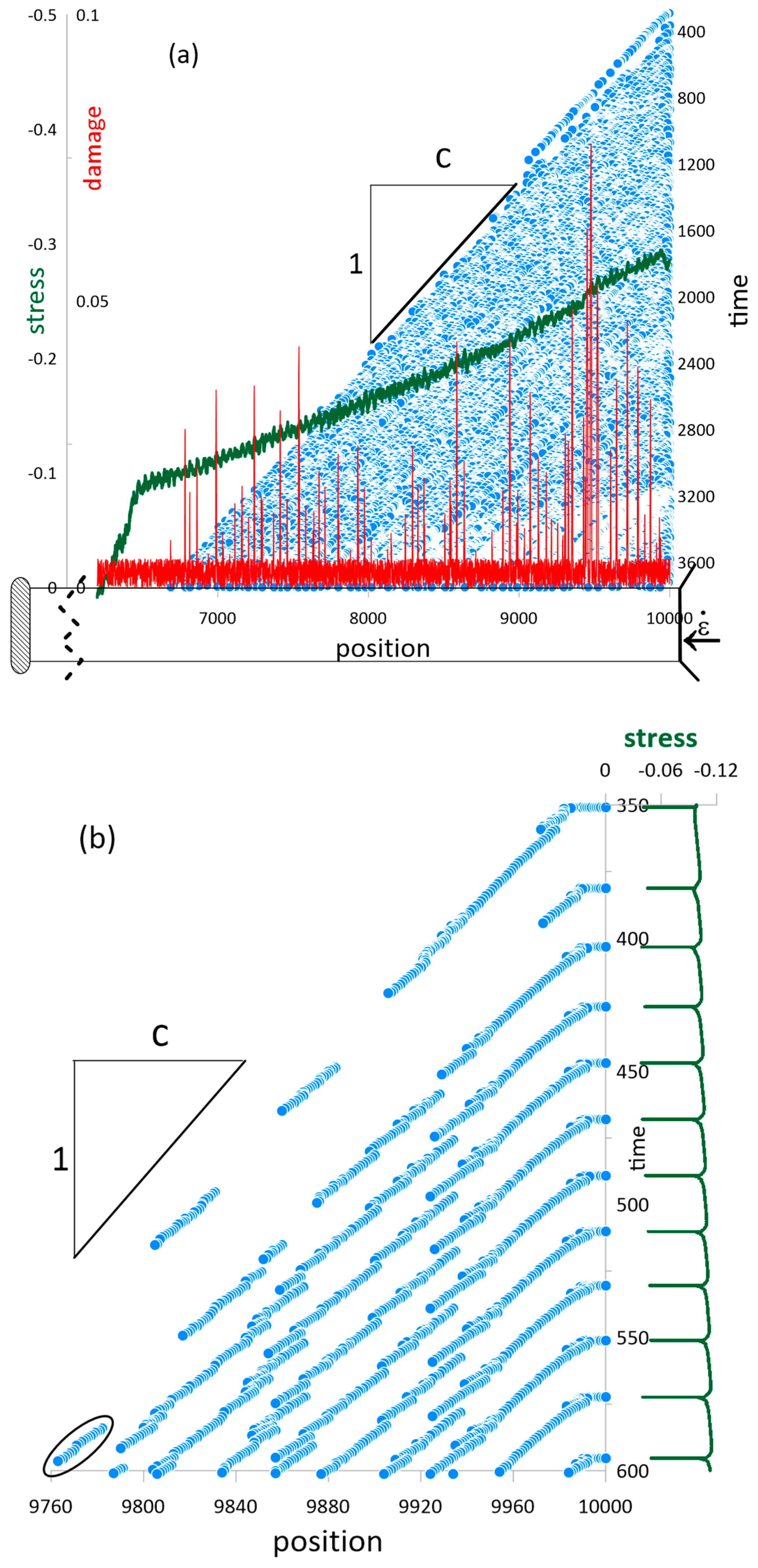
• Dislocation emission events are local unloadings of representative volumes.
• In physical space, DEEs self-organize into slip bans and avalanches.
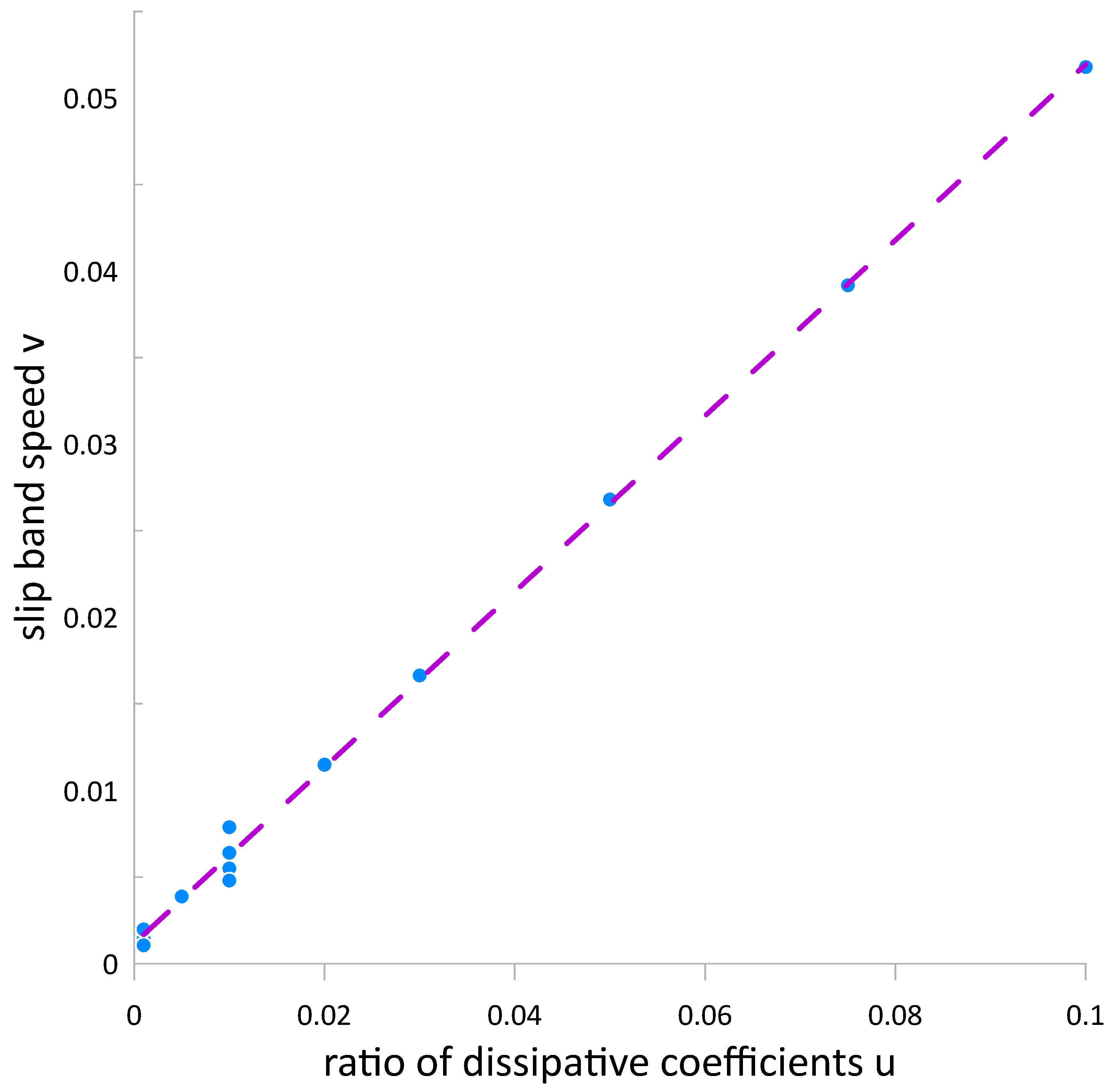
• Speed of slip band propagation is $v=\gamma \sqrt{\mu {\kappa }_{\omega }}\vartheta \left(\epsilon \right)$.
• Dislocation avalanches propagate at a speed higher than the speed of sound.
• In the deformation phase space, DEEs take place on the yield surface.

References

1. Zaiser, M. Scale invariance in plastic flow of crystalline solids. Adv. Phys. 2006, 55, 185–245. [Google Scholar] [CrossRef]
2. Papanikolaou, S.; Cui, Y.; Ghoniem, N. Avalanches and plastic flow in crystal plasticity: An overview. Model. Simul. Mater. Sci. Eng. 2018, 26, 013001. [Google Scholar] [CrossRef]
3. Dimiduk, D.M.; Woodward, C.; LeSar, R.; Uchic, M.D. Scale-free intermittent flow in crystal plasticity. Science 2006, 312, 1188–1190. [Google Scholar] [CrossRef] [PubMed]
4. Rizzardi, Q.; McElfresh, C.; Sparks, G.; Stauffer, D.D.; Marian, J.; Maaß, R. Mild-to-wild plastic transition is governed by athermal screw dislocation slip in bcc Nb. Nat. Commun. 2022, 13, 1010. [Google Scholar] [CrossRef] [PubMed]
5. Alcalá, J.; Očenášek, J.; Varillas, J.; El-Awady, J.A.; Wheeler, J.M.; Michler, J. Statistics of dislocation avalanches in FCC and BCC metals: Dislocation mechanisms and mean swept distances across microsample sizes and temperatures. Sci. Rep. 2020, 10, 19024. [Google Scholar] [CrossRef] [PubMed]
6. Weiss, J.; Grasso, J.-R.; Miguel, M.-C.; Vespignani, A.; Zapperi, S. Complexity in dislocation dynamics: Experiments. Mater. Sci. Eng. 2001, A309–310, 360–364. [Google Scholar] [CrossRef]
7. Weiss, J.; Marsan, D. Three-dimensional mapping of dislocation avalanches: Clustering and space/time coupling. Science 2003, 299, 89–92. [Google Scholar] [CrossRef] [PubMed]
8. Weiss, J.; Richeton, T.; Louchet, F.; Chmelík, F.; Dobroň, P.; Entemeyer, D.; Lebyodkin, M.; Lebedkina, T.; Fressengeas, C.; McDonald, R.J. Evidence for universal intermittent crystal plasticity from acoustic emission and high-resolution extensometry experiments. Phys. Rev. 2007, B76, 224110. [Google Scholar] [CrossRef]
9. Ispánovity, P.D.; Ugi, D.; Péterffy, G.; Knapek, M.; Kalácska, S.; Tuzes, D.; Dankházi, Z.; Máthis, K.; Chmelík, F.; Groma, I. Dislocation avalanches are like earthquakes on the micron scale. Nat. Commun. 2022, 13, 1975. [Google Scholar] [CrossRef] [PubMed]
10. Bulatov, V.V.; Cai, W. Computer Simulations of Dislocations, Oxford Series on Materials Modeling; Sutton, A.P., Rudd, R.E., Eds.; Oxford University Press: Oxford, UK, 2006. [Google Scholar]
11. Kubin, L. Dislocations, Mesoscale Simulations and Plastic Flow; Oxford Series on Materials Modeling; Sutton, A.P., Rudd, R.E., Eds.; Oxford University Press: Oxford, UK, 2013. [Google Scholar]
12. Miguel, M.-C.; Vespignani, A.; Zapperi, S.; Weiss, J.; Grasso, J.-R. Intermittent dislocation flow in viscoplastic deformation. Nature 2001, 410, 667–671. [Google Scholar] [CrossRef] [PubMed]
13. Berdichevsky, V.L. Beyond classical thermodynamics: Dislocation-mediated plasticity. J. Mech. Phys. Solids 2019, 129, 83–118. [Google Scholar] [CrossRef]
14. Csikor, F.F.; Motz, C.; Weygand, D.; Zaiser, M.; Zapperi, S. Dislocation Avalanches, Strain Bursts, and the Problem of Plastic Forming at the Micrometer Scale. Science 2007, 318, 251–254. [Google Scholar] [CrossRef] [PubMed]
15. Devincre, B.; Hoc, T.; Kubin, L. Dislocation Mean Free Paths and Strain Hardening of Crystals. Science 2008, 320, 1745–1748. [Google Scholar] [CrossRef] [PubMed]
16. Chan, P.Y.; Tsekenis, G.; Dantzig, J.; Dahmen, K.A.; Goldenfeld, N. Plasticity and dislocation dynamics in a phase field crystal model. Phys. Rev. Lett. 2010, 105, 015502. [Google Scholar] [CrossRef] [PubMed]
17. Koslowski, M.; LeSar, R. Thomson R Avalanches and scaling in plastic deformation. Phys. Rev. Lett. 2004, 93, 125502. [Google Scholar] [CrossRef] [PubMed]
18. Umantsev, A. Bifurcation Theory of Plasticity, Damage and Failure. Mater. Today Comm. 2021, 26, 102121, Corrigendum in Mater. Today Comm. 2023, 37, 107377. [Google Scholar] [CrossRef]
19. Umantsev, A. Thermodynamically Consistent Model of Dislocation-Mediated Plasticity. Phil. Mag. Part A Mater. Sci. 2024, 105, 2408383. [Google Scholar] [CrossRef]
20. Umantsev, A. Multiscale Theory of Dislocation Plasticity. J. Mater. Sci. Mater. Theory, 2025; to be submitted. [Google Scholar]
21. Mayergoyz, I.D. Mathematical Models of Hysteresis; Springer: Berlin, Germany, 1991. [Google Scholar]
22. Landau, L.D.; Lifshitz, E.M. Theory of Elasticity; Pergamon Press: Oxford, UK, 1970. [Google Scholar]
Figure 1. Quasistatic stress–damage–strain diagram of loading and unloading. Y—point of yielding; U—point of unloading; DEE—dislocation emission event; arrows—direction of deformation.
Metals 15 00626 g001
Figure 2. Equilibrium state diagram of an ideal plastic specimen with free-energy density, Equation (8), in the phase space (z, ω). Green line—elastic state; blue line—plastic state; brown line—barrier state; vertical dash dot—yielding; red dot—DEEs in creep compression; red line—DEEs in shock compression.
Metals 15 00626 g002
Figure 3. Time series of dislocation emission events (blue dots) and internal (thermodynamic) stress (green line) in the regime of creep loading.
Metals 15 00626 g003
Figure 4. Probability density function of dislocation emission events measured by the free-energy change in the compressive creep regime of loading. Blue dots—binned DEEs. Pink line—linear fit of the ‘mild’ part of the emission events.
Metals 15 00626 g004
Figure 5. (a) Space–time map of DEEs. v —slip band speed. Left insert: slip bands. Right insert: quiet zone. (b) Distribution of strain (blue), back strain (brown), stress (green), and damage (red) in the plastically deformed part of the specimen.
Metals 15 00626 g005
Figure 6. Distributions of strain (blue), stress (green), and damage (red) in the train wave of dislocation emission events. (a) Space distributions in a slip band at t = 25,000. (b) Time distributions in a representative volume at x = 9900.
Metals 15 00626 g006
Figure 7. Scaled speed (blue dots) of slip band propagation, v , as a function of the ratio of dissipative coefficients, u , for the constant strain rate, ε ˙ . Dash line—scaled expression by Equation (22b).
Metals 15 00626 g007
Figure 8. Time series of dislocation emission events (blue dots) and internal (thermodynamic) stress (green), damage (red), and back strain (brown) in shock loading.
Metals 15 00626 g008
Figure 9. Probability distribution function of dislocation emission events measured by the free-energy change in the shock compression regime of loading. Blue dots—binned DEEs. Pink line—linear fit of DEEs.
Metals 15 00626 g009
Figure 10. Energy balance in the specimen. Green line—external work of loading; brown line—total emissions by the specimen; blue line—total free energy of the specimen.
Metals 15 00626 g010
Figure 11. Space–time map of dislocation emission events in a shock-loaded specimen. (a) Blue dots—DEEs; green line—distribution of stress; red line—distribution of damage. (b) High resolution of the first 600 time-units of (a). Green line—stress on the loaded end of the specimen. (c) Damage structure of the avalanche marked by an oval in (b).
Metals 15 00626 g011aMetals 15 00626 g011b
Figure 12. Time series of stress (green), damage (red), and strain (blue) in the first three slip bands at the loaded end of the specimen.
Metals 15 00626 g012
Figure 13. Stress–damage–strain diagram for shock loading. Blue arrow—loading direction.
Metals 15 00626 g013