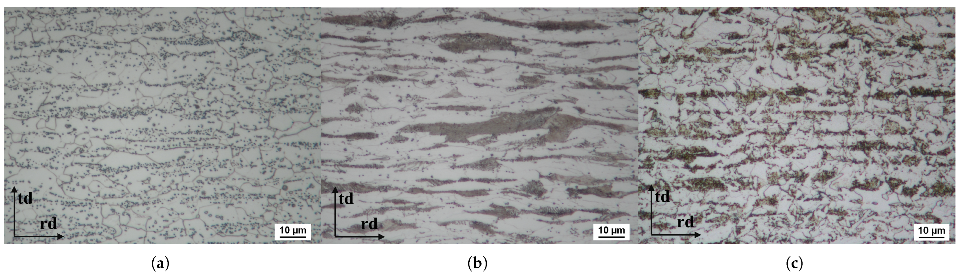
Article

Investigating the Tensile Properties of 22MnB5 After Austenitization and Quenching with Different Initial Microstructures

1
Division of Solid Mechanics, Luleå University of Technology, 971 87 Luleå, Sweden
2
Gestamp Hardtech AB, Technology and Innovation Office, Ektjärnsvägen 5, 973 45 Luleå, Sweden
*
Author to whom correspondence should be addressed.
Metals 2025, 15(6), 589; https://doi.org/10.3390/met15060589
Submission received: 22 April 2025 / Revised: 16 May 2025 / Accepted: 22 May 2025 / Published: 25 May 2025

Abstract

In the automotive industry, structural components are often produced via press hardening, enabling rapid production and the use of ultra-high-strength steels. In this process, steels are heated to an austenitic state and are then formed and quenched in rapid succession. The initial steel that enters the press-hardening production line varies, where the microstructure is a result of previous production steps. This work was performed to investigate the possible effects of the initial microstructure on the final mechanical properties for rapidly quenched samples. Although the initial microstructure is transformed during austenitization, the steel can still be affected by its prior history. Steels with three different initial microstructures were evaluated, with only minor variations in chemical composition and thicknesses. The Lankford coefficients and the failure strains were dependent on the orientation of the samples. However, for a given orientation, there were only minor variations between the different steels with respect to anisotropy, strength, and ductility. The anisotropy could be correlated with the microstructure through the calculation of Taylor factors based on measurements using electron backscatter diffraction. The minor influence from the initial steel microstructure on the final mechanical properties indicates robustness suitable for mass production.

1. Introduction

Using press hardening, it is possible to produce a wide range of components, with varying degrees of complexity, using low-carbon steel containing modest amounts of alloying elements. This method traditionally utilizes two distinct thermal events: austenitization and quenching. The production cycle begins with a steel blank that is heated until it reaches an austenitic state and is then formed and quenched using pressing tools. The technology has widespread use in the automotive industry for a multitude of reasons: the components can be produced to obtain a final ultimate stress that exceeds 2 GPa [1], and the steels are relatively inexpensive and recyclable. Another positive aspect is the design freedom achieved by combining the formability of austenite at elevated temperatures with ultra high strength in the final component. Bumper beams, B-pillars, and other structural parts where strength is essential are often produced using the press-hardening technique. A more thorough description of the process and its applications can be found in works by Karbasian and Tekkaya [2] and Wróbel et al. [3].
Depending on the sheet thickness used to produce a component, the steel can either be hot-rolled or cold-rolled. Further, the steel can have a surface coating applied at the steel mill or be subjected to additional heat treatments. The evolution of the microstructure begins with liquid metal, which is continuously cast and formed into sheet metal through rolling operations. During hot rolling of the class of steels used in this study, the microstructure is composed of austenite, which recrystallizes during the operation. Traces of the earlier production steps might be observed in the form of a banded microstructure [4]. During cold rolling, a previously hot rolled steel sheet is further reduced in thickness through additional rolling steps at a lower temperature, which creates a microstructure containing elongated grains. The steel exhibits increased yield and tensile stresses but at the expense of reduced ductility. The microstructure of both hot and cold rolled variants is mainly composed of ferrite and pearlite. The steel can undergo additional production steps, e.g., soft annealing, in order to reduce strength and increase ductility. This can be useful to reduce tool wear and the forces involved during forming or cutting operations. During the soft annealing of low carbon steels, the cementite lamellae in pearlite transforms into a spherical form, and the ferrite is recrystallized. Low-carbon steels are usually not soft-annealed in order to improve machinability, as the microstructure becomes too soft [5].
The specific grade studied within this work is 22MnB5, which is a commonly utilized press-hardening steel. It is available in several different as-delivered states with varying strength levels, and will, after press hardening, exhibit a tensile strength in the region of 1400–1600 MPa. The steel has a low carbon content and is alloyed with manganese and boron. The martensite start temperature is relatively high, around 400 °C, allowing autotempering. Therefore, the steel is not reliant on dedicated tempering processes to achieve the desired mechanical properties. The coating process commonly used in the automotive industry does, however, have an effect on the tensile properties due to a curing step at an elevated temperature [6], which is typically accounted for in research by heating the samples to 170 °C for 20 min.
Although the initial microstructure will be transformed during austenitization, it might affect the mechanical properties of the finished component. One possible effect is variations in austenite morphology, which in turn influence the final microstructure after quenching. The austenite transformation is dependent on numerous factors, e.g., the initial microstructure and the heating rate. Azizi-Alizamini et al. [7] studied the formation of austenite in hot and cold rolled steels, where the differences in the transformation behavior and austenite morphology between the two steels were found to be dependent on the heating rate. Golem et al. [8] and Zheng et al. [9] studied the effect of the austenitization parameters on the final mechanical properties using press-hardenable steels, finding a larger effect for notched tensile samples as compared to straight samples. The influence of the initial microstructure on the properties of 22MnB5 after press hardening have previously been evaluated by Järvinen et al. [6,10], finding an effect on the tensile properties by the initial microstructure. The differences in strength with respect to the initial microstructure were affected by a paint baking treatment, which involved heating the steels to 170 °C for 20 min.
During the production of components, further variations occur due to nesting optimization, where the blank is cut from the original steel in a specific orientation to minimize the amount of scrap produced. Anisotropy related to the rolling direction might thus arise and have to be taken into consideration for press-hardened components. One measure of anisotropy in sheet metals is the strain ratio r = ε w i d t h / ε t h i c k , originally proposed by Lankford et al. [11]. The initial application was to evaluate the deep drawing properties of a material, and has since been found to be a convenient parameter for material models. Examples include the works by Hill and Orowan [12], Barlat et al. [13], and Hu et al. [14], where strain ratios can be related to model parameters. The anisotropy of low-carbon boron steels at elevated temperatures have previously been studied by Turetta et al. [15], where two different effective measures based on the r-values were evaluated. The weighted average plastic strain ratio was found to be temperature-dependent and the degree of planar anisotropy was minor for all temperatures. These two effective measures can be found in ISO 10113:2020 [16] and will be defined in Section 2.3. However, the testing was performed during cooling at elevated temperatures, which differs from the work within this article. Eller [17] measured the r-values for 5 different press-hardened conditions at room temperature, finding variations for a majority of the conditions with respect to the rolling directions. The mechanical properties can also be affected by non-metallic inclusions, which are inherited from earlier production steps. An example is manganese sulfides, which are formed during continuous casting and further elongated during the rolling operations. The mechanical properties perpendicular to the rolling direction are negatively affected by manganese sulfide inclusions [18].
Variations in the microstructure of the steels will invariably exist; therefore, it is important that the effect of the initial microstructure is understood. It has previously been established that the strength of press-hardened 22MnB5 exhibits variations with respect to the initial microstructure [6,10]. This study furthers the previously conducted research by also evaluating the ductility and anisotropy for different orientations with respect to the rolling direction. Using steels with three different initial microstructures, tensile testing is performed with measurements using digital image correlation (DIC) and a physical extensometer. Strength, ductility, and anisotropic properties, defined via the r-values, are evaluated using both monotonic and cyclic loading schemes. Two similar boron steels are utilized, one cold-rolled and the other hot-rolled. Further, a subset of the cold-rolled steel is soft annealed in order to produce a third initial microstructure. The study is limited to rapidly quenched samples, with an ultimate tensile strength close to 1.5 GPa. Electron backscatter diffraction (EBSD) is used to evaluate the final microstructure as well as to reconstruct the parent austenite microstructure.

2. Materials and Methods

2.1. Materials

Three different steels were used in the experiments, the first produced through hot rolling (HR), as well as two steels where the final thickness was achieved through cold rolling. The cold-rolled steel was used both in an as-rolled state (CR) and in a spherodized state, which will be referred to as cold rolled and soft annealed (CR + SA). The chemical compositions of the steels are shown in Table 1. The spherodization was achieved by annealing the steel for 24 h at 700 °C, where ten samples with dimensions of 180 mm × 60 mm were wrapped in stainless foil and heated while argon gas was supplied to protect the steel. After 24 h, the furnace was turned off and the steel was left to cool slowly within the furnace for a duration of 18 h, after which the samples had reached 130 °C and were removed from the furnace. The microstructure of the hot-rolled, cold-rolled, and the soft-annealed steel can be seen in Figure 1. The microstructures were revealed using a 3% Nital etchant solution, and the images were captured using light optical microscopy.

2.2. Austenitization and Quenching

Tensile test specimens according to Figure 2 were cut from the three steels, oriented at angles of 0°, 45°, and 90° with respect to the rolling direction. The large radius of 7250 mm was added to the 60 mm long parallel length to ensure localization within the measuring length of the extensometer.
The samples were heated in a Nabertherm muffle furnace (Nabertherm GmbH, Lilienthal, Germany) set to 930 °C, while the sample temperature was measured using a K-type thermocouple. The samples were kept in the furnace for 200 s, counted from when the measured sample temperature reached 915 °C. After 200 s, the samples were quenched in oil to 50 °C, resulting in a cooling rate of 80 °C/s for the majority of the quenching. The thermal cycle for one of the samples can be seen in Figure 3. After quenching, the samples were heated to 170 °C for 20 min to account for paint-baking effects.

2.3. Tensile Testing

Tensile testing was performed using a Dartec M1000/RK (Dartec Ltd., Bournemouth, UK) servo-hydraulic universal testing machine, where the crosshead speed was set to 0.1 mm/s. The deformation was measured with an extensometer with an initial measuring length of 50 mm, as well as using an ARAMIS DIC system (Carl Zeiss GOM Metrology GmbH, Braunschweig, Germany). The hardware and software settings for the DIC measurements are summarized in Table 2. The area that was monitored consisted of the region within the span of the physical extensometer, with the parts closest to the edge excluded. A visualization of the measurement area can be seen in Figure 4, and also visible in the same figure are the strain variations at the point of maximum force.
Three tensile tests using monotonic loading were performed for each combination of the three steels (HR, CR, and CR + SA) and three different orientations (0°, 45°, and 90°), giving a total of 27 tests. For each combination of steel and orientation, one cyclic tensile test was also performed. The cyclic loading was performed as follows:
  • Application of a 1.4 mm crosshead displacement.
  • Unloading to a tensile load of 1.0 kN.
  • Pause for 1 s.
  • Capturing an image with the DIC system.
  • Return to step 1.
The cyclic loading scheme enabled the direct calculation of the plastic strain using the DIC-system close to an unloaded state. A comparison of the monotonic and cyclic loading schemes can be seen in in Figure 5.
The failure strain was measured both as the total elongation using the extensometer and the local strain at failure calculated by DIC. The local failure strain was defined as the largest von-Mises equivalent strain found in the localized area in the last frame before a visible fracture or crack appears.
The anisotropy was evaluated by calculating the Lankford coefficients for each specimen orientation. The measurement was originally defined by Lankford et al. [11] as
r = ε w ε t ,
where r is the strain ratio, and ε w and ε t are the strain components in the width and thickness directions, respectively. The definitions of these strains can be found in the standards ISO 10113:2020 [16] and ASTM E517-19 [19]. Both standards specify similar measurement methodologies using either extensometers, manual measurements of an unloaded sample, or a mix of the two methods for ISO 10113:2020 [16]. The elastic strain is to be deducted using Young’s modulus and Poisson’s ratio according to both standards if extensometer measurements are utilized. By using digital image correlation, the strain was calculated continuously over the entire measurement area instead of using extensometers. The strain components used to calculate the r-value were averaged over the entire measurement area; these area-averaged strain components will hereafter be denoted by the bar sign as ε ¯ . DIC has previously been used to study the r-value; Anderson and Raeisinia [20] calculated the r-value locally and later averaged this over the region of interest, in addition the authors also used virtual extensometers to measure the strain. Marth et al. [21] calculated the r-value locally and averaged the values based on the local effective plastic strain. Yu et al. [22] used DIC to calculate the average strain over the entire measurement area and used these average strains to calculate the r-value. The last approach was also used in this study. A further example is the Finite element model updating method, which was used by Denys et al. [23] in combination with DIC to determine model parameters directly, without explicitly calculating the r-values.
In this study, the r-value was calculated both as a function of strain increments, as well as a cumulative measure between 1% and 3% plastic strain. The incremental calculation was performed assuming plastic incompressibility as
r θ i = ε ¯ w p ε ¯ t p ε ¯ w p , i ε ¯ w p , i 1 ε ¯ t p , i ε ¯ t p , i 1 = ε ¯ w p , i ε ¯ w p , i 1 ε ¯ w p , i + ε ¯ l p , i + ε ¯ w p , i 1 + ε ¯ l p , i 1 ,
where r θ i is the strain ratio at an angle θ toward the rolling direction at the sampling point i, and ε ¯ w p , i , ε ¯ t p , i , and ε ¯ l p , i are the plastic strains in the width, thickness, and lengthwise directions. Using the strain calculations from the DIC measurements and the force, the following expressions were used to subtract the elastic strains:
ε ¯ w p , i ε ¯ w i + ν σ ¯ l i / E ,
ε ¯ l p , i ε ¯ l i σ ¯ l i / E ,
where ε ¯ w i and ε ¯ l i are the total strains in the width and lengthwise directions; σ ¯ l i is the average stress in the lengthwise direction; and E and ν are the Young’s modulus and Poisson’s ratio, which were assumed to be 200 GPa and 0.3, respectively. The average stress σ ¯ l i in the lengthwise direction can be calculated from the instantaneous force F i and true strain according to
σ ¯ l i = F i / A i = F i exp ε ¯ l i / A 0 ,
where A i and A 0 are the instantaneous and initial cross-sectional areas. This equation where the cross-sectional area is calculated from the true strain is based on an assumption of uniform strain and is therefore not valid after the onset of necking.
The incremental strain as defined in Equation (2) was calculated between each DIC sampling point, with the exception of the cyclic tests. For these, the incremental strain was only calculated between the unloaded states. Due to noise in the calculated strain increments, a moving average filter was used for the plastic strain components, where the four closest neighbors before and after each data point were included. The total number of data points for the monotonic loading varied between 94 and 115, depending on the specific test. This filtering was not needed for the samples that were tested with a cyclic load due to the larger strain increments. To quantify the difference between the different steels, three effective measures from ISO 10113:2020 [16] were calculated. First was the mean r-value between 1% and 3% plastic strain in the lengthwise direction, r θ / 1 3 , according to the regression method in the standard, where the r-value is defined as
r θ / 1 3 = b 1 + b ,
where b is the slope of a linear approximation describing the relationship between the plastic strain in the width and length directions. The data points closest to 1% and 3% plastic strain were used to fit the linear function. The weighted average plastic strain ratio was calculated as
r ¯ = r 0 / 1 3 + 2 r 45 / 1 3 + r 90 / 1 3 4 ,
which is also sometimes called the normal plastic anisotropy ratio; see, e.g., [24]. Finally, the degree of planar anisotropy was calculated as
Δ r = r 0 / 1 3 + r 90 / 1 3 2 r 45 / 1 3 2 .

2.4. EBSD-Analysis

EBSD analysis was performed to correlate the anisotropic plastic behavior seen in the tensile testing with the microstructure. The Lankford coefficients can be approximated from the EBSD-data through the calculation of the Taylor factors. A virtual strain increment is applied in the tensile direction, leading to contraction in the width and thickness direction to preserve the volume. The Lankford coefficient can then be approximated as the ratio between these two strains that minimize the Taylor factor; see Bunge [25]. The polycrystalline behavior was assumed to be the sum of a weighted Taylor factor for each grain, where the weight for each grain was the grain area. This algorithm is implemented in the MTEX software [26] as the function calcLankford. The complex microstructure of martensite does not exhibit grains in the classical sense; therefore, the grains were represented by regions with a misorientation of 3°. The r-value was varied in increments of 0.01, leading to a difference in the strain tensor used to calculate the Taylor factor. To calculate the Taylor factor, the slip systems have to be defined, which were assumed to be {1 1 0}〈1 1 1〉 and {1 1 2}〈1 1 1〉. The critical resolved shear stress (CRSS) was set to unity for both classes of slip systems. In the EBSD-data, the parent austenite grains were reconstructed through the variant graph approach, utilizing the orientation relationships between martensite and the prior austenite microstructure. This method is described in the work by Hielscher et al. [27] and is implemented in MTEX. Post-processing of the EBSD-data was performed using MTEX 6.0.0 and MatLab 2024b (Mathworks, Inc., Natick, MA, USA). A modification was introduced to the calcLankford function, where the definition of the thickness direction was changed to align with the tensile samples.
The samples were cut from undeformed areas of three tensile test specimens. The samples were mounted, ground, polished, and vibratory-polished. Scanning was performed using a Zeiss Gemini SEM (Carl Zeiss Microscopy GmbH, Jena, Germany) with an Oxford symmetry EBSD-detector (Oxford Instruments, Abingdon, UK). The normal of the scanned area was aligned with the rolling direction. The accelerating voltage was 15 kV, the step size was 0.18 μm, and the total size of the scanned area was 275 μm × 367 μm.

3. Results

3.1. Tensile Properties

The r-values calculated using Equations (6)–(8) can be seen in Table 3, and the continuously calculated r-values can be seen in Figure 6. The elongation measured via the physical extensometer, the local fracture strain retrieved from the DIC-system, and the tensile strength can be seen in Table 4 and Table 5. The engineering stress versus engineering strain curves are presented in Figure 7, where the strain was acquired from the physical extensometer.

3.2. EBSD-Analysis

The calculated Taylor factors as a function of r-values can be viewed in Figure 8, where the values have been normalized for visualization purposes. The r-values, the minimum Taylor factors, and average parent austenite grain size for each steel can be seen in Table 6. Inverse polar figure (IPF) maps of the martensitic microstructure and the reconstructed parent austenite grains can be seen in Figure 9. The regions in the aforementioned figure represents a cropped subsection of the scanned area with the dimensions of 100 μm × 100 μm. The thickness and width directions of the original steel coil are aligned with the vertical and horizontal axes of the images, respectively. The grain size distribution of the reconstructed parent austenite grains can be seen in Figure 10.

4. Discussion

Tensile testing of samples produced using steels with three different initial microstructures yielded similar stress–strain curves after austenitization and quenching, with the hot-rolled steel having slightly higher flow stress. Common for the three steels was the anisotropic behavior, both in the form of a reduced elongation in the direction transverse to the rolling direction and a variation in the r-values. In an industrial sense, the reduction in ductility might be of greater importance compared to a minor plastic anisotropy. The reason for this loss in ductility is probably due to elongated non-metallic inclusions. However, the variations between the different steels, for a given orientation (0°, 45° or 90°), were minor. The calculation of the incremental r-values suggested constant anisotropy with increasing plastic strain up to necking, aligning well with the regression method utilized to calculate the cumulative r-value according to ISO 10113:2020 [16]. The small differences between the different steels indicate a robustness of the production process, which might be advantageous during large volume production, where the initial microstructure can vary. Furthermore, the consistent behavior simplifies the material modeling needed when evaluating the properties of the final component, e.g., crashworthiness performance. The results are in line with the previously published work by Järvinen et al. [6,10], where the tensile properties were evaluated for the same steel grade, 22MnB5. However, the specific microstructures studied, the chemical compositions of the steels and the heat treatments employed differ slightly compared to this study. The differences in ultimate tensile strength between the steels with different initial microstructures were slightly smaller than those reported by Järvinen et al. [6] for samples that had undergone a paint-baking treatment. This study showed that these differences in strength are irrespective of the rolling direction, and that the elongation, anisotropy, and local failure strain also only display minor variations with respect to the initial microstructure.
The slight anisotropic properties reveal that the steels are influenced by the prior production processes and are not reset during austenitization. The differences were consistent for all three evaluated initial microstructures and are thus seemingly unaffected by both cold rolling and soft annealing of the initial steel. The estimated r-values calculated from the EBSD-data suggests that the behavior is due to a slightly textured microstructure. The absolute values of r-values measured during tensile testing and the calculations from EBSD-data reveal minor differences. However, the overall trend is the same with the 0° samples having the lowest r-values and the 45° having the highest r-values, with the exception of the soft-annealed sample aligned at 90° with respect to the rolling direction. A change in the available slip systems used for the calculations only has a minor effect on the r-value estimation. The chosen method to measure the austenitization time, starting at 915 °C, generated similar parent austenite grain sizes for the different steels. The average value of the grain size was greatly affected by the presence of many small grains in the reconstructed austenite.
The cyclic loading, which was performed using spare samples, was intended to compare the measurements of loaded and unloaded samples. As the r-value is based on plastic strains, it is possible to either measure the plastic strains directly in an unloaded state or subtract the elastic strains from measurements of a loaded sample. Both approaches are valid according to ISO 10113:2020 [16] and ASTM E517-19 [19]. Except for one steel and orientation (HR 0°), the r-values calculated from the unloaded strain field using cyclic loading was higher. This variation should be noted as both methodologies are valid according to previously mentioned standards. In one instant (HR 45°), the failure strain retrieved from the DIC-system indicated a larger value for the cyclic loading compared to monotonic loading. Due to the single specimen used for the cyclic testing, it is hard to draw any conclusion due to the scatter in experimental work. This specific sample localized very close to the end of the parallel length, where the sample was slightly wider, which might have a minor effect on the local strain.
It must also be noted that even though the research was aimed at further understanding the press-hardening process, the samples were quenched using submersion in oil and not using a pressing tool. The cooling rate, which was around 80 °C/s, should ensure a fully martensitic microstructure similar to what is achieved in industry [28].

5. Conclusions

The three different steels that were part of this study were hardened through austenitization and rapid quenching. Given the results of tensile testing of these steels, the authors have drawn the following conclusions:
  • The initial microstructure had a limited effect on the tensile properties for samples with a specific orientation with respect to the rolling direction.
  • Variations of the Lankford coefficients depending on the orientation of the tensile samples were observed.
  • The ductility transverse to the rolling direction was equally reduced for the steels with three different initial microstructures.
  • The austenitization and quenching of the evaluated steels produced very consistent mechanical properties.
  • The anisotropic behavior measured during tensile testing aligned well with the r-values estimated using EBSD-data. Although the absolute values vary between the two methods, the trends are similar.
All conclusions based on the results in this work are limited to rapidly quenched samples. If the samples had been cooled at a lower rate, the phase composition could differ between samples, leading to variations in mechanical properties. Further studies are to be performed using varying cooling rates, thus extending the understanding of the influence of the initial microstructure to a more general case. Also, in order to model the entire press-hardening production, one must consider how the surface of the initial steel reflects heat, as heating through radiation is important during austenitization. The measured heating rate during the experiments did not reveal any major differences between the different steels. However, the samples were austenitized in an atmosphere of air. A more inert atmosphere might affect the rate of oxidation, and thus the reflectivity, emissivity, transmissivity, and absorptivity of the samples. The furnace atmosphere can also influence the decarburization of the surface layer for uncoated steels, which could affect the final mechanical properties, especially the bending properties. As press-hardening is often used for components undergoing large deformations during collisions, a failure model is needed. The tensile testing performed within this work, where the elongation and local fracture strain were measured, would have to be complemented with other sample geometries to capture a wider range of stress states.

Author Contributions

Conceptualization, E.L.; formal analysis, E.L.; investigation, E.L.; project administration, P.Å.; supervision, J.K. and P.Å.; visualization, E.L.; writing—original draft, E.L.; writing—review & editing, J.K. and P.Å. All authors have read and agreed to the published version of the manuscript.

Funding

The research presented in this article was part of the PROCHAIN project, with funding provided by Gestamp Hardtech AB through the Centre for High performance Steels, CHS, at Luleå University of Technology.

Data Availability Statement

The raw data supporting the conclusions of this article will be made available by the authors on request.

Acknowledgments

The authors would like to thank Gestamp Hardtech AB for the ability to utilize their laboratory facilities and their contribution of technical expertise, and SSAB for the supply of material and for technical support. Finally, the authors would like to extend their gratitude to Jan Granström, Khalifa Maissara, Lars Frisk, and Erik Nilsson at Luleå University of Technology for valuable insights and help with the experimental work. The EBSD-scanning was performed by Swerim AB.

Conflicts of Interest

Authors Erik Lundholm and Paul Åkerström were employed by the company Gestamp Hardtech AB. The remaining author declares that the research was conducted in the absence of any commercial or financial relationships that could be construed as a potential conflict of interest.

Abbreviations

The following abbreviations are used in this manuscript:
DICDigital image correlation.
EBSDElectron backscatter diffraction.
HRHot rolled.
CRCold rolled.
CR + SACold rolled and soft annealed.
CRSSCritical resolved shear stress.
IPFInverse polar figure.

References

  1. Taylor, T.; McCulloch, J. Effect of Part/Die Boundary Conditions on Microstructural Evolution during Hot Stamping 2000 MPa Class Boron Steel. Steel Res. Int. 2018, 89, 1700495. [Google Scholar] [CrossRef]
  2. Karbasian, H.; Tekkaya, A.E. A review on hot stamping. J. Mater. Process. Technol. 2010, 210, 2103–2118. [Google Scholar] [CrossRef]
  3. Wróbel, I.; Skowronek, A.; Grajcar, A. A Review on Hot Stamping of Advanced High-Strength Steels: Technological-Metallurgical Aspects and Numerical Simulation. Symmetry 2022, 14, 969. [Google Scholar] [CrossRef]
  4. Krauss, G. Steels: Processing, Structure, and Performance, 2nd ed.; ASM International: Almere, The Netherlands, 2015; pp. 184–187. [Google Scholar]
  5. Holm, T.; Olsson, P.; Troell, E. (Eds.) Stål Och Värmebehandling: En Handbok; Swerea IVF: Mölndal, Sweden, 2010; pp. 333–336. [Google Scholar]
  6. Järvinen, H.; Honkanen, M.; Järvenpää, M.; Peura, P. Effect of paint baking treatment on the properties of press hardened boron steels. J. Mater. Process. Technol. 2018, 252, 90–104. [Google Scholar] [CrossRef]
  7. Azizi-Alizamini, H.; Militzer, M.; Poole, W.J. Austenite Formation in Plain Low-Carbon Steels. Metall. Mater. Trans. A 2011, 42, 1544–1557. [Google Scholar] [CrossRef]
  8. Golem, L.; Cho, L.; Speer, J.G.; Findley, K.O. Influence of austenitizing parameters on microstructure and mechanical properties of Al-Si coated press hardened steel. Mater. Des. 2019, 172, 107707. [Google Scholar] [CrossRef]
  9. Zheng, X.; Ghassemi-Armaki, H.; Hartwig, K.T.; Srivastava, A. Correlating Prior Austenite Grain Microstructure, Microscale Deformation and Fracture of Ultra-High Strength Martensitic Steels. Metals 2021, 11, 1013. [Google Scholar] [CrossRef]
  10. Järvinen, H.; Isakov, M.; Nyyssönen, T.; Järvenpää, M.; Peura, P. The effect of initial microstructure on the final properties of press hardened 22MnB5 steels. Mater. Sci. Eng. A 2016, 676, 109–120. [Google Scholar] [CrossRef]
  11. Lankford, W.T.; Snyder, S.C.; Bauscher, J.A. New criteria for predicting the press performance of deep drawing sheets. Trans. Am. Soc. Met. 1950, 42, 1197–1232. [Google Scholar]
  12. Hill, R.; Orowan, E. A theory of the yielding and plastic flow of anisotropic metals. Proc. R. Soc. Lond. Ser. A Math. Phys. Sci. 1948, 193, 281–297. [Google Scholar] [CrossRef]
  13. Barlat, F.; Brem, J.C.; Yoon, J.W.; Chung, K.; Dick, R.E.; Lege, D.J.; Pourboghrat, F.; Choi, S.H.; Chu, E. Plane stress yield function for aluminum alloy sheets—Part 1: Theory. Int. J. Plast. 2003, 19, 1297–1319. [Google Scholar] [CrossRef]
  14. Hu, Q.; Chen, J.; Yoon, J.W. A new asymmetric yield criterion based on Yld 2000-2d under both associated and non-associated flow rules: Modeling and validation. Mech. Mater. 2022, 167, 104245. [Google Scholar] [CrossRef]
  15. Turetta, A.; Bruschi, S.; Ghiotti, A. Anisotropic and Mechanical Behavior of 22MnB5 in Hot Stamping Operations. AIP Conf. Proc. 2007, 907, 217–222. [Google Scholar] [CrossRef]
  16. ISO 10113:2020; Metallic Materials—Sheet and Strip—Determination of Plastic Strain Ratio. International Organization for Standardization: Geneva, Switzerland, 2020.
  17. Eller, T. Modeling of Tailor Hardened Boron Steel for Crash Simulation. Ph.D. Thesis, University of Twente, Enschede, The Netherlands, 2016. [Google Scholar] [CrossRef]
  18. Maciejewski, J. The Effects of Sulfide Inclusions on Mechanical Properties and Failures of Steel Components. J. Fail. Anal. Prev. 2015, 15, 169–178. [Google Scholar] [CrossRef]
  19. ASTM E517-19; Standard Test Method for Plastic Strain Ratio r for Sheet Metal. ASTM International: West Conshohocken, PA, USA, 2019.
  20. Anderson, D.; Raeisinia, B. Micro and Macro Analysis of Anisotropy of an AA3104 Aluminum Alloy. IOP Conf. Ser. Mater. Sci. Eng. 2018, 418, 012088. [Google Scholar] [CrossRef]
  21. Marth, S.; Djebien, S.; Kajberg, J.; Häggblad, H.Å. Stepwise modelling method for post necking characterisation of anisotropic sheet metal. Model. Simul. Mater. Sci. Eng. 2021, 29, 085001. [Google Scholar] [CrossRef]
  22. Yu, K.; Hou, L.; Guo, M.; Li, D.; Huang, D.; Zhuang, L.; Zhang, J.; Wu, P. A method for determining r-value of aluminum sheets with the Portevin-Le Chatelier effect. Mater. Sci. Eng. A 2021, 814, 141246. [Google Scholar] [CrossRef]
  23. Denys, K.; Coppieters, S.; Seefeldt, M.; Debruyne, D. Multi-DIC setup for the identification of a 3D anisotropic yield surface of thick high strength steel using a double perforated specimen. Mech. Mater. 2016, 100, 96–108. [Google Scholar] [CrossRef]
  24. Marciniak, Z.; Duncan, J.L.; Hu, J. Mechanics of Sheet Metal Forming, 2nd ed.; Butterworth-Heinemann: Oxford, UK, 2002; p. 9. [Google Scholar]
  25. Bunge, H.J. 13—Physical Properties of Polycrystalline Materials. In Texture Analysis in Materials Science; Bunge, H.J., Ed.; Butterworth-Heinemann: Oxford, UK, 1982; pp. 330–338. [Google Scholar] [CrossRef]
  26. MTEX. Available online: https://mtex-toolbox.github.io/ (accessed on 9 December 2024).
  27. Hielscher, R.; Nyyssönen, T.; Niessen, F.; Gazder, A.A. The variant graph approach to improved parent grain reconstruction. Materialia 2022, 22, 101399. [Google Scholar] [CrossRef]
  28. Bardelcik, A.; Salisbury, C.P.; Winkler, S.; Wells, M.A.; Worswick, M.J. Effect of cooling rate on the high strain rate properties of boron steel. Int. J. Impact Eng. 2010, 37, 694–702. [Google Scholar] [CrossRef]
Figure 1. The initial microstructure of the three different steels, showing (a) the cold-rolled and soft-annealed steel and (b) the cold-rolled steel and (c) the hot-rolled steel. The vertical axis (td) denotes the thickness direction, and the horizontal axis (rd) denotes the rolling direction.
Metals 15 00589 g001
Figure 2. Geometry of the tensile test specimens used, where all measurements are defined in mm.
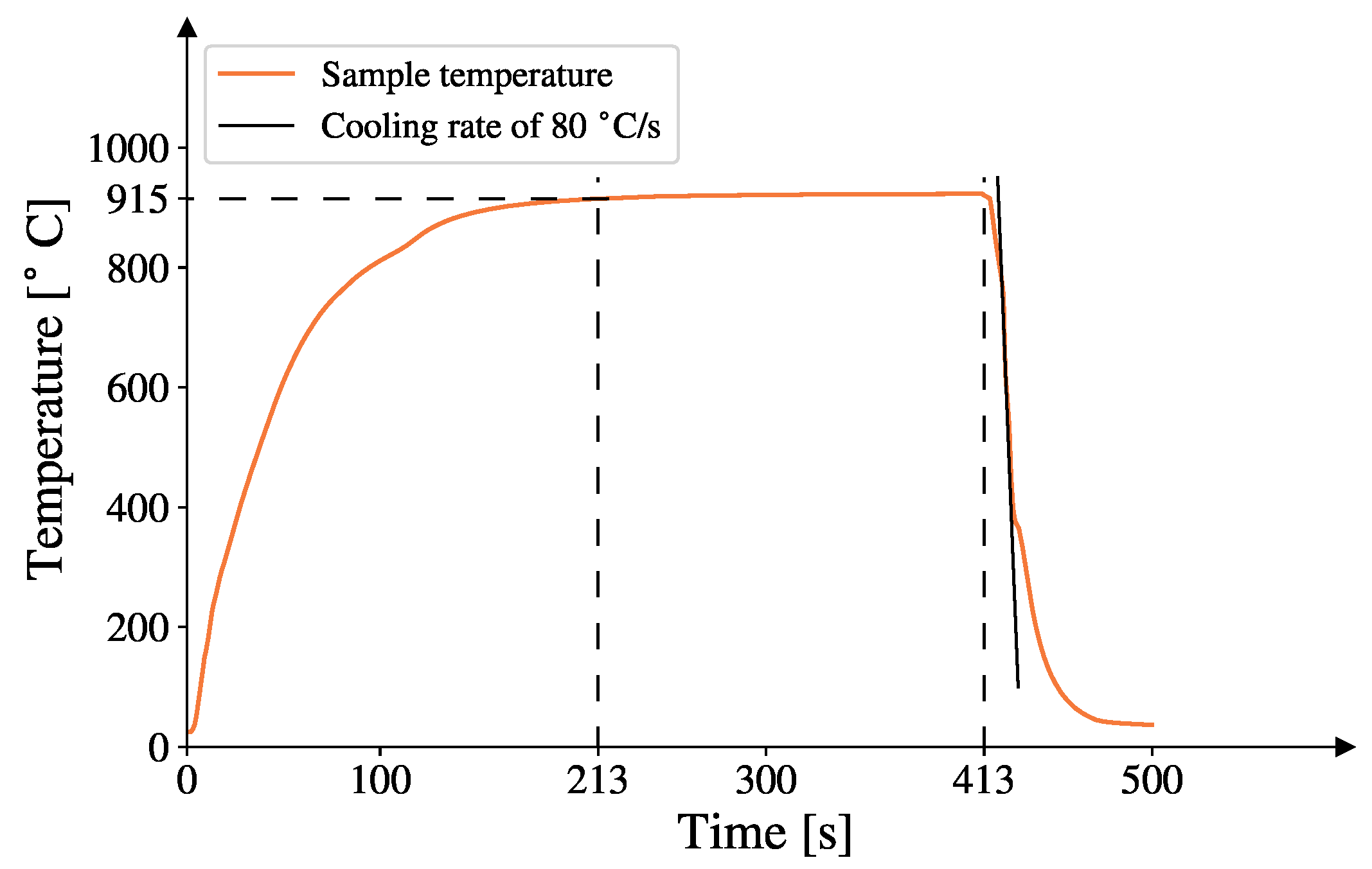
Metals 15 00589 g002
Figure 3. Representative thermal cycle of the austenitization and quenching, where the dashed lines show the start of the austenitization period (at 213 s) when the samples reached 915 °C and the stop of the austenitization period (at 413 s). Also included is a tangent displaying the cooling rate.
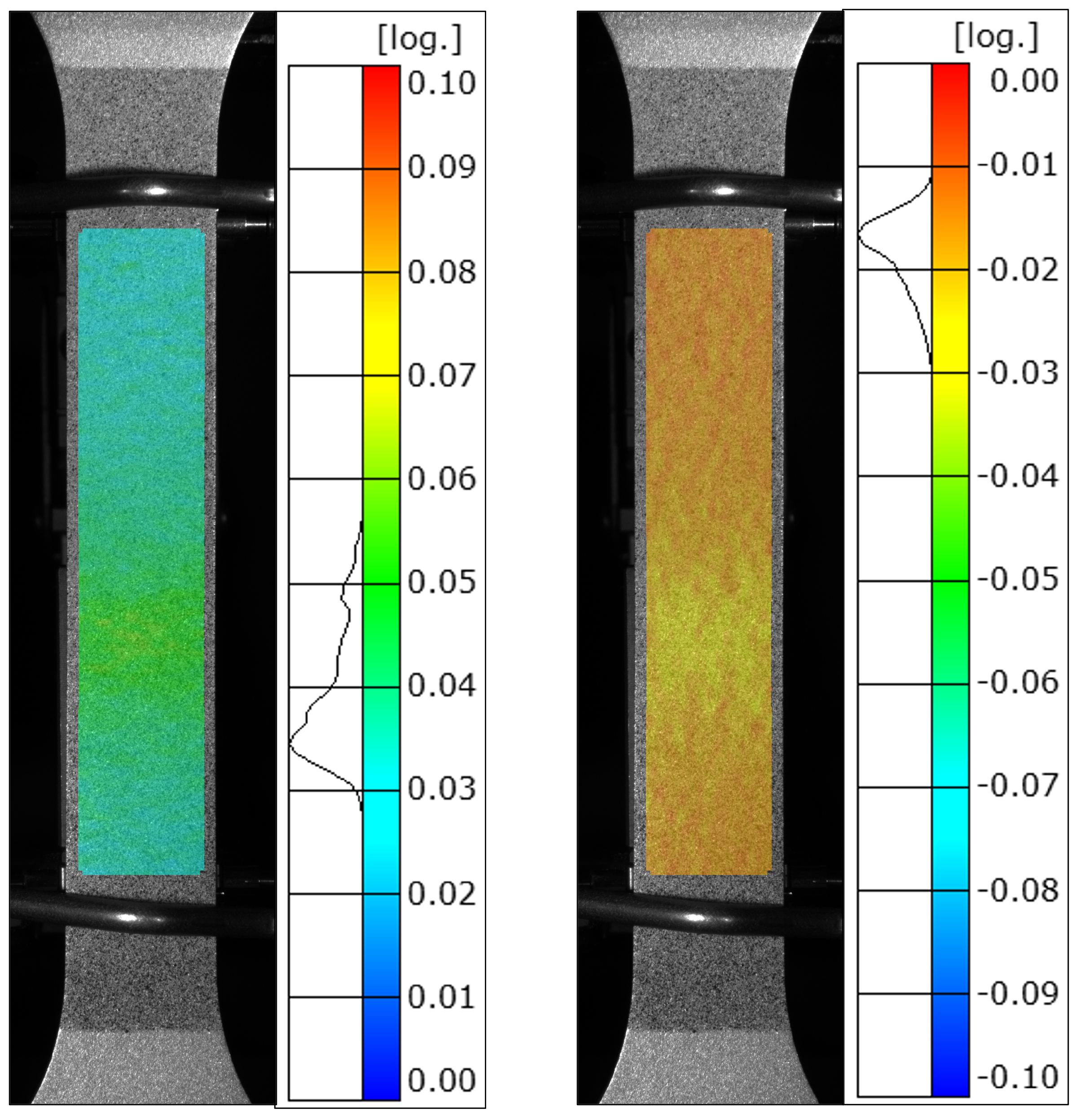
Metals 15 00589 g003
Figure 4. Visualization of the measurement area used for the strain calculations. Also visible are the strain distributions in the lengthwise direction (left) and width direction (right) at the point of maximum force during tensile testing.
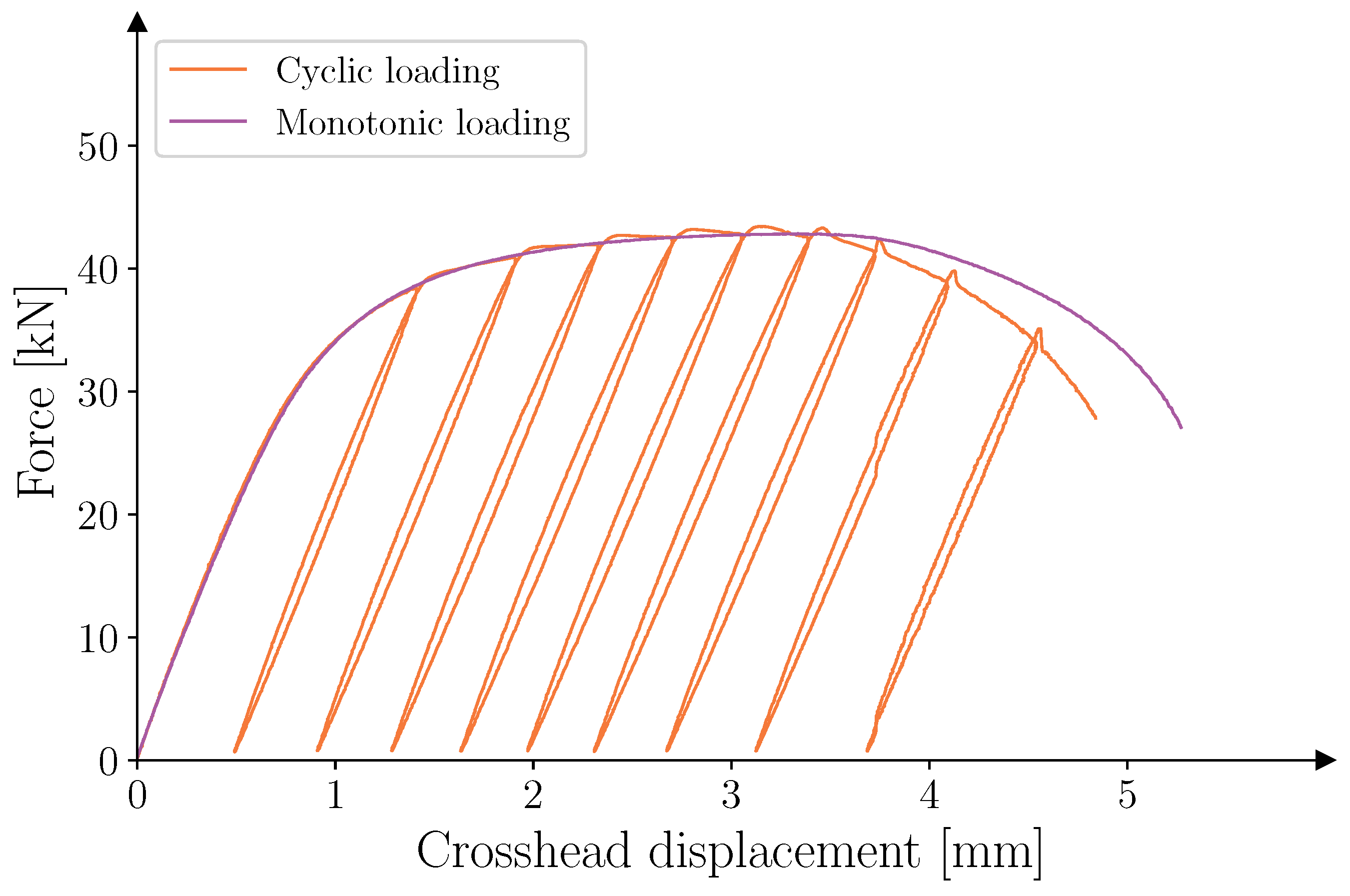
Metals 15 00589 g004
Figure 5. Comparison of the monotonic and cyclic loading schemes used in tensile testing.
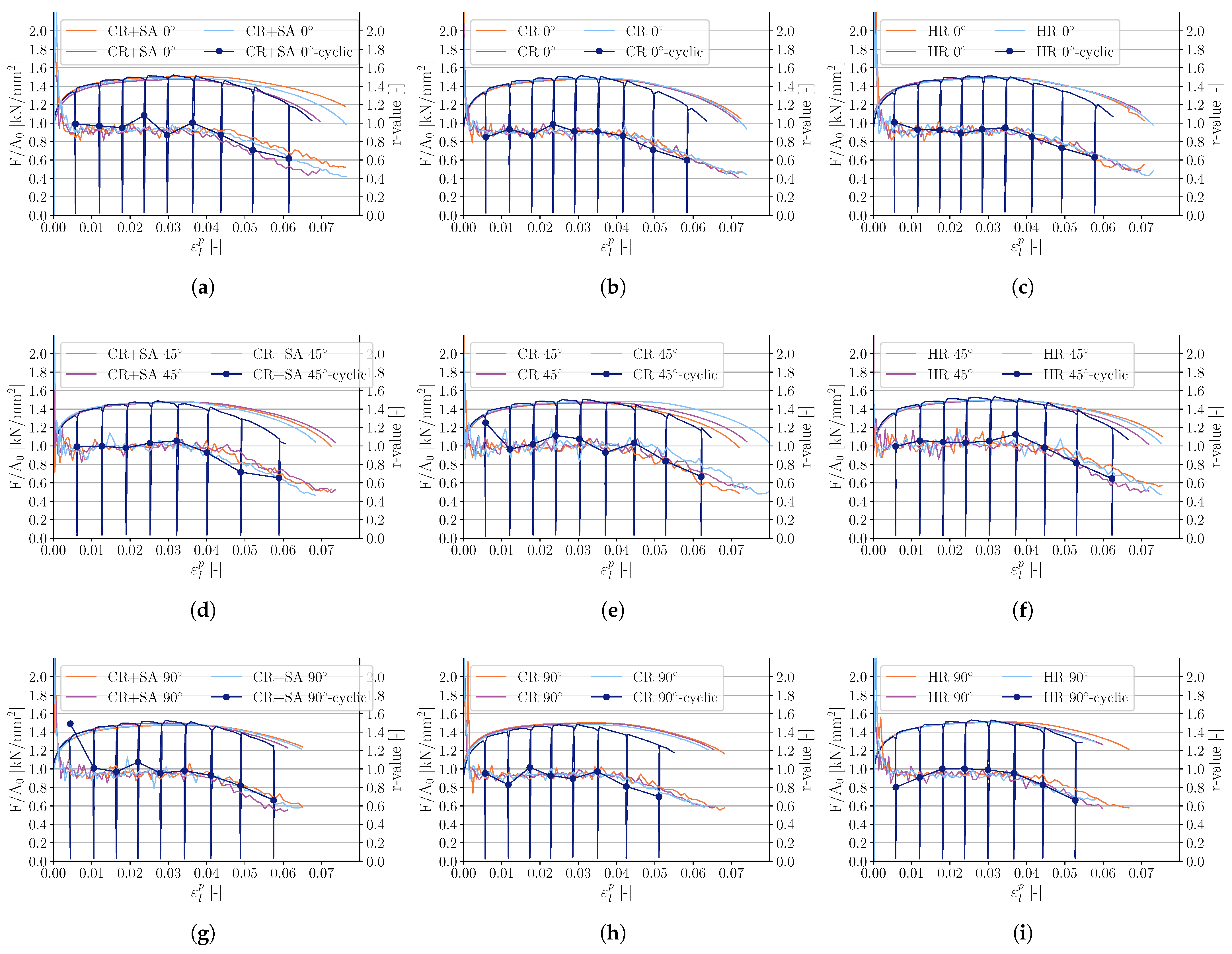
Metals 15 00589 g005
Figure 6. r-values and engineering stress as a function of plastic strain for the (a) cold-rolled and soft-annealed steel oriented at 0°, (b) cold-rolled steel oriented at 0°, (c) hot-rolled steel oriented at 0°, (d) cold-rolled and soft-annealed steel oriented at 45°, (e) cold-rolled steel oriented at 45°, (f) hot-rolled steel oriented at 45°, (g) cold-rolled and soft-annealed steel oriented at 90°, (h) cold-rolled steel oriented at 90°, and (i) hot-rolled steel oriented at 90°.
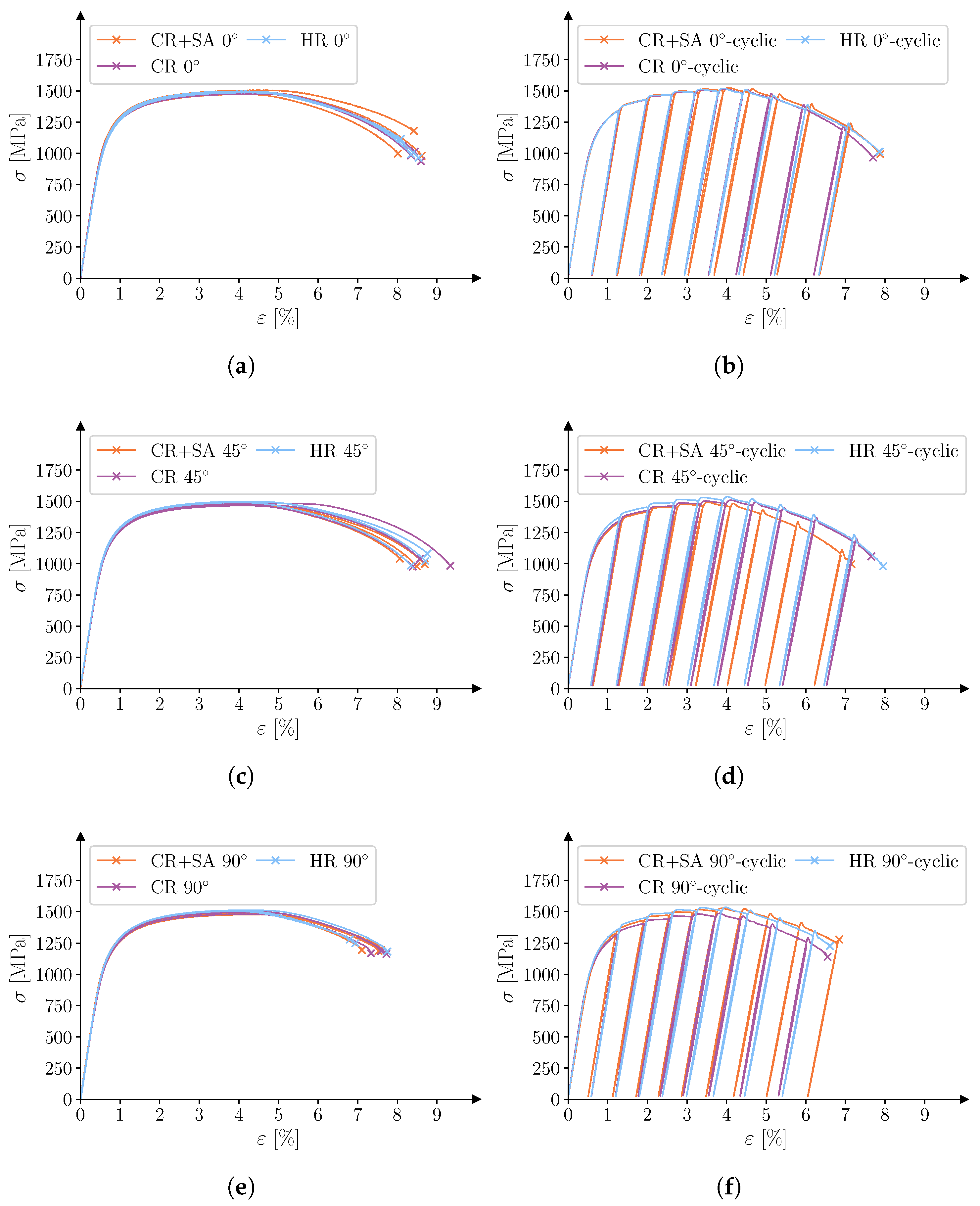
Metals 15 00589 g006
Figure 7. Engineering stress and engineering strain for (a) monotonic loading oriented at 0° with respect to the rolling direction, (b) cyclic loading oriented at 0° with respect to the rolling direction, (c) monotonic loading oriented at 45° with respect to the rolling direction, (d) cyclic loading oriented at 45° with respect to the rolling direction, (e) monotonic loading oriented at 90° with respect to the rolling direction, and (f) cyclic loading oriented at 90° with respect to the rolling direction.
Metals 15 00589 g007
Figure 8. Normalized Taylor factors as a function of the r-value for (a) the cold-rolled and soft-annealed steel, (b) the cold-rolled steel, and (c) the hot-rolled steel.
Metals 15 00589 g008
Figure 9. IPF maps of the final martensitic microstructure (ac) and the reconstructed parent austenite grains (df). The vertical and horizontal axes of the images are aligned with the thickness and width directions of the original steel coil, respectively.
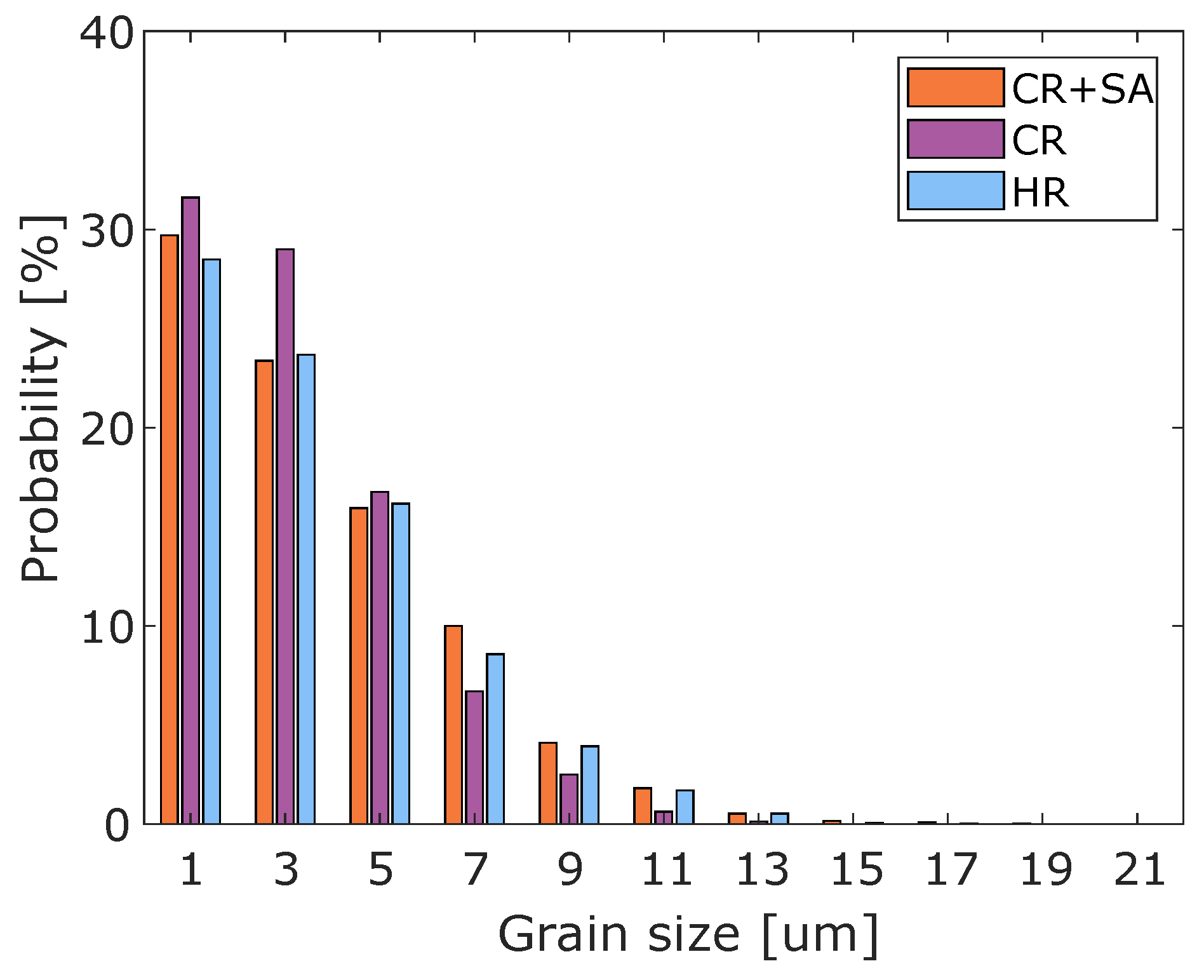
Metals 15 00589 g009
Figure 10. Grain size distribution of the reconstructed parent austenite microstructure.
Metals 15 00589 g010
Table 1. Mass percentage of the alloy elements in the evaluated steels measured using optical emission spectroscopy. The primary element is Fe.
Initial ConditionCSiMnPSCrB
CR/CR + SA0.2150.2631.1700.0140.0020.1910.004
HR0.2290.2671.2300.0110.0020.2160.004
Table 2. Software settings and hardware used for measurements and strain calculations.
DIC Measurement and Processing Setup
CameraGOM Aramis 5M
LensNikkor AF 24 mm f/2.8 D (Nikon Corporation, Tokyo, Japan)
Image scale [mm/px]0.04
Image acquisition rate [Hz]2 (monotonic loading) 1 (cyclic loading)
Patterning techniqueSpray paint
SoftwareGOM Aramis V6.3
Subset size [px]21 × 21
Subset step [px]8
Subset shapeQuadratic
Points used in strain calculation [-]3 × 3
Strain definitionTotal strain, Logarithmic
Table 3. r-values for each combination of steel and orientation. For the samples that were monotonically loaded, the average results are presented, as well as the minimum and maximum values within the parentheses.
Initial Conditionr0/1–3 [-]r45/1–3 [-]r90/1–3 [-] r ¯ [-]Δr [-]
CR + SA0.92 (0.92–0.93)0.99 (0.99–1.01)0.95 (0.94–0.96)0.96−0.06
CR0.91 (0.90–0.91)1.00 (0.98–1.01)0.93 (0.93–0.94)0.96−0.08
HR0.92 (0.92–0.92)1.02 (1.02–1.03)0.94 (0.93–0.94)0.98−0.09
CR + SA, cyclic test0.971.021.001.00−0.04
CR, cyclic test0.931.070.941.00−0.14
HR, cyclic test0.911.041.001.00−0.09
Table 4. Failure strain for the three different steels, where ε θ A 50 is the total elongation and ε θ v m is the local von-Mises strain retrieved from the DIC system. For the samples that were monotonically loaded, the results are the average of the three samples. The minimum and maximum values are included within the parentheses.
Initial Condition ε 0 A 50 [%] ε 0 v m [%] ε 45 A 50 [%] ε 45 v m [%] ε 90 A 50 [%] ε 90 v m [%]
CR + SA8.35 (8.01–8.61)77.1 (65.5–89.0)8.41 (8.06–8.69)81.5 (78.6–85.4)7.41 (7.11–7.59)49.8 (47.5–51.5)
CR8.46 (8.35–8.60)79.9 (75.6–83.7)8.77 (8.39–9.34)85.3 (83.0–89.8)7.55 (7.34–7.72)54.1 (51.9–58.0)
HR8.32 (8.09–8.54)78.4 (68.9–86.8)8.60 (8.34–8.76)77.1 (73.1–80.2)7.16 (6.80–7.75)48.1 (43.6–54.1)
CR + SA, cyclic7.8881.87.1579.26.8449.8
CR, cyclic7.7076.97.6677.36.5553.8
HR, cyclic7.8674.57.9581.26.6145.1
Table 5. The average tensile strength for the samples that were monotonically loaded, with the minimum and maximum values presented within the parentheses.
Initial Condition R m , 0 [MPa] R m , 45 [MPa] R m , 90 [MPa]
CR + SA1489 (1475–1506)1478 (1473–1480)1487 (1478–1500)
CR1484 (1477–1490)1473 (1466–1483)1494 (1482–1503)
HR1494 (1487–1498)1495 (1491–1500)1509 (1503–1512)
Table 6. The r-values r θ , the minimum Taylor factors M θ , m i n , and the average parent austenite grain size D a v g . The r-values measured during tensile testing with monotonic loading are included as a comparison within the parentheses.
Initial Condition r 0 [-] M 0 , m i n [-] r 45 [-] M 45 , m i n [-] r 90 [-] M 90 , m i n [-] D a v g [µm]
CR + SA0.96 (0.92)2.8241.01 (0.99)2.7981.05 (0.95)2.8034.1
CR0.95 (0.91)2.8271.03 (1.00)2.7931.00 (0.93)2.8163.7
HR0.97 (0.92)2.8001.02 (1.02)2.7961.01 (0.94)2.8033.9
Disclaimer/Publisher’s Note: The statements, opinions and data contained in all publications are solely those of the individual author(s) and contributor(s) and not of MDPI and/or the editor(s). MDPI and/or the editor(s) disclaim responsibility for any injury to people or property resulting from any ideas, methods, instructions or products referred to in the content.

