
Material Characterisation, Modelling, and Validation of a UHSS Warm-Forming Process for a Heavy-Duty Vehicle Chassis Component


Abstract
1. Introduction
2. Materials and Methods
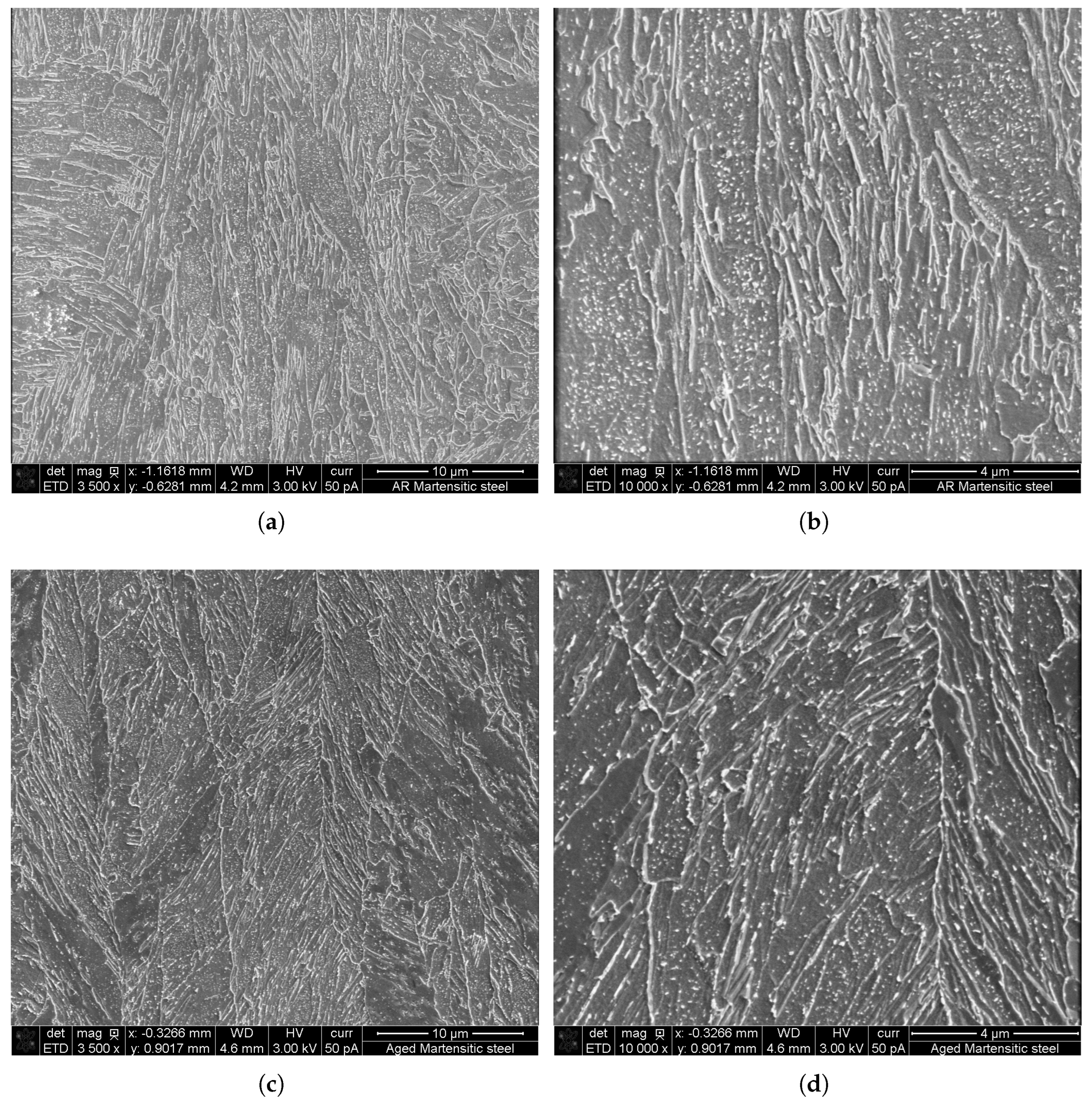
2.1. Ultra-High Strength Steel for Warm Forming
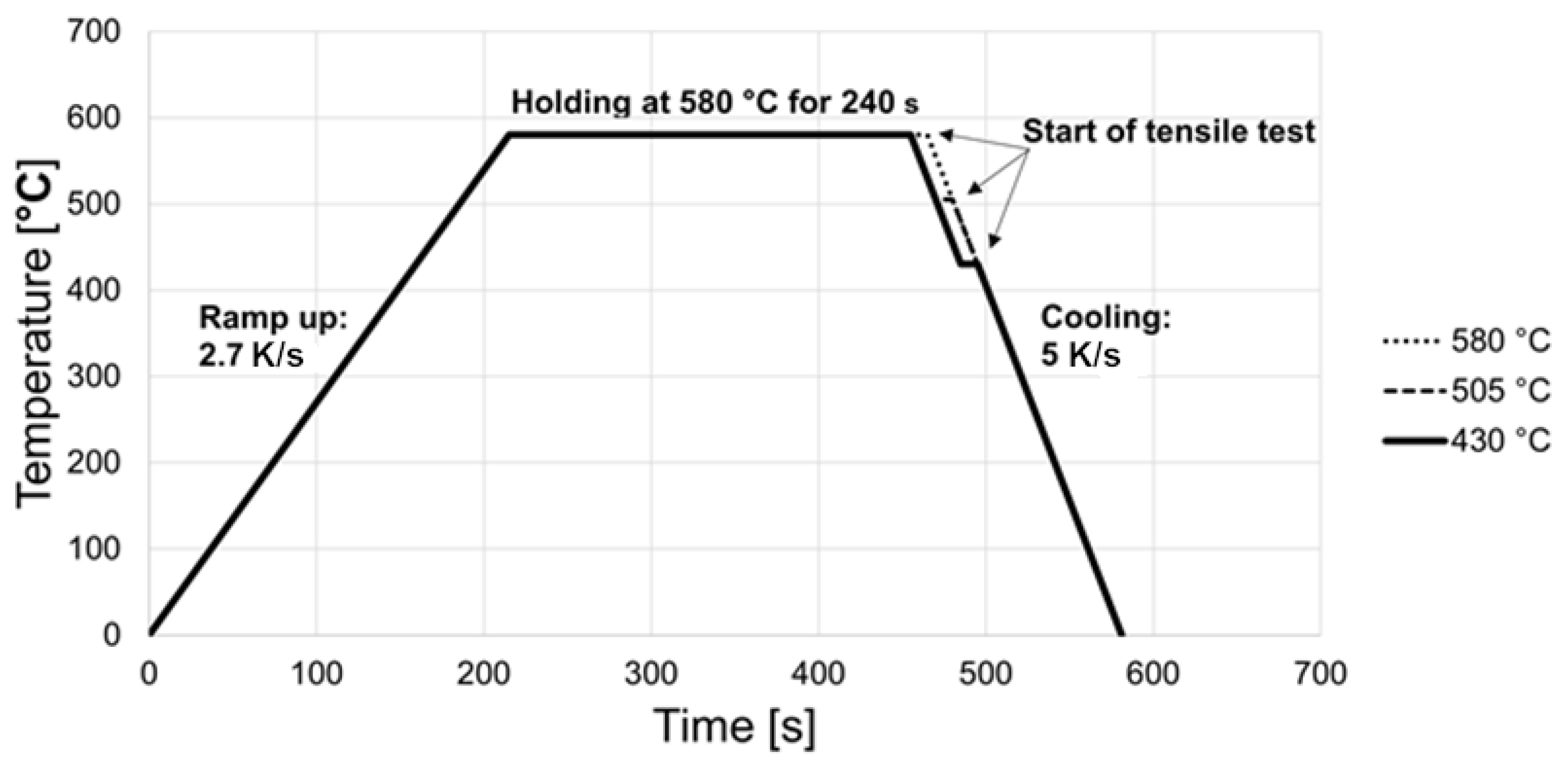
Thermal History
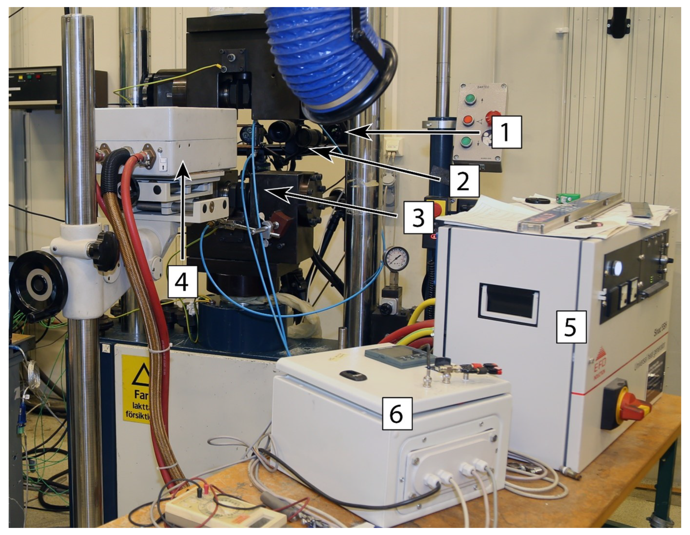
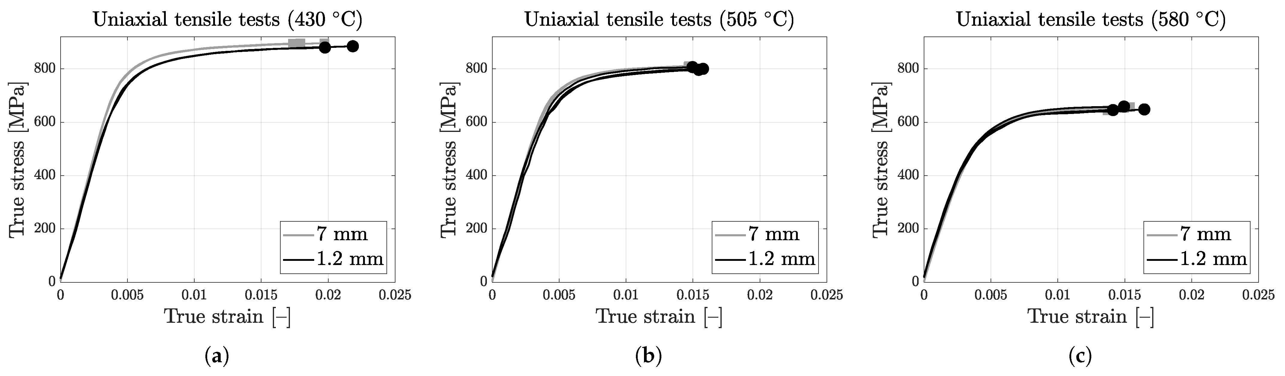
2.2. Experiments
- Thickness reduction investigation;
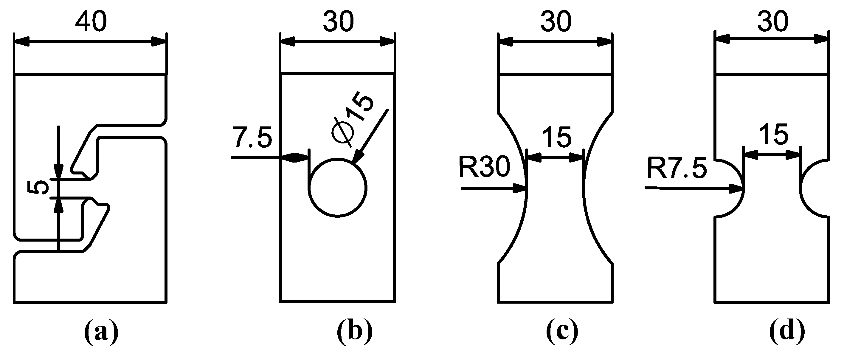
- Plasticity/fracture property investigation;
- Young’s modulus investigation.
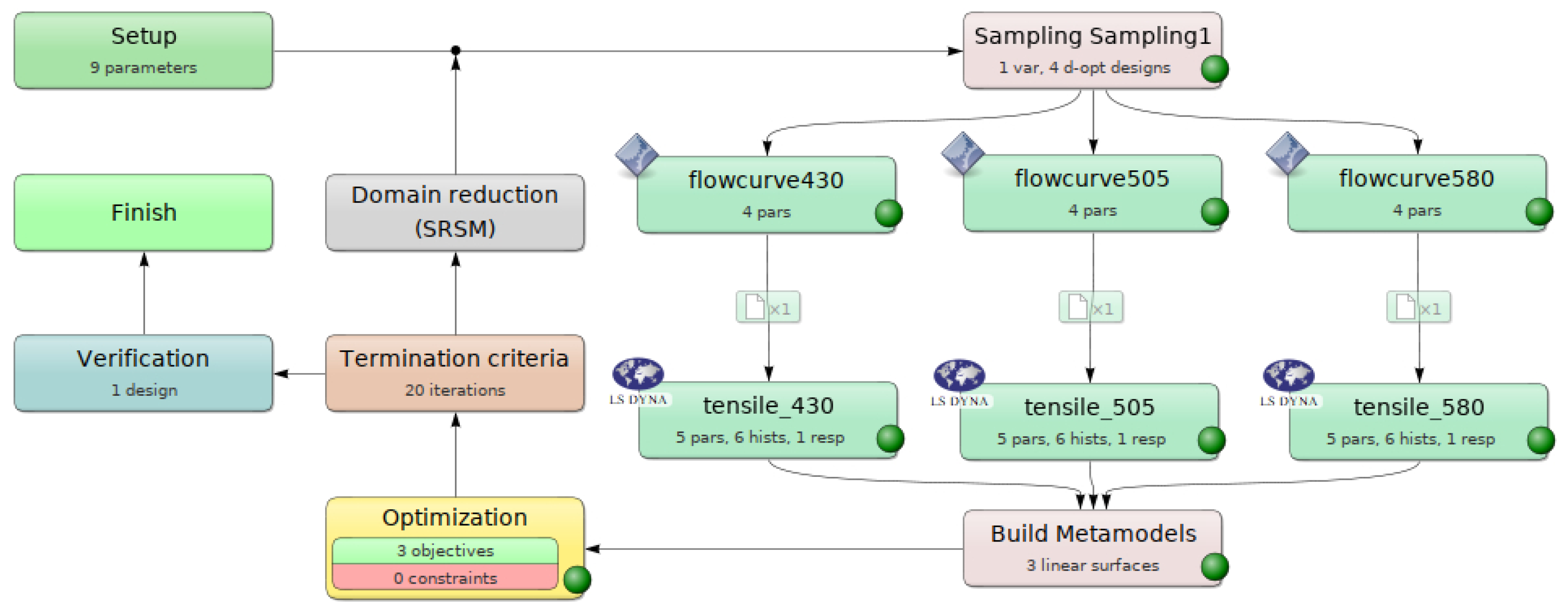
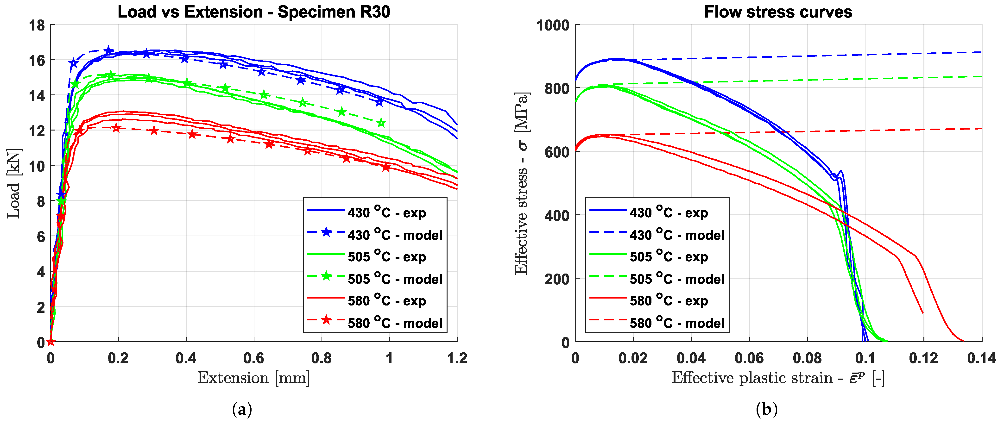
2.3. Calibration of Temperature Dependent Work-Hardening Model
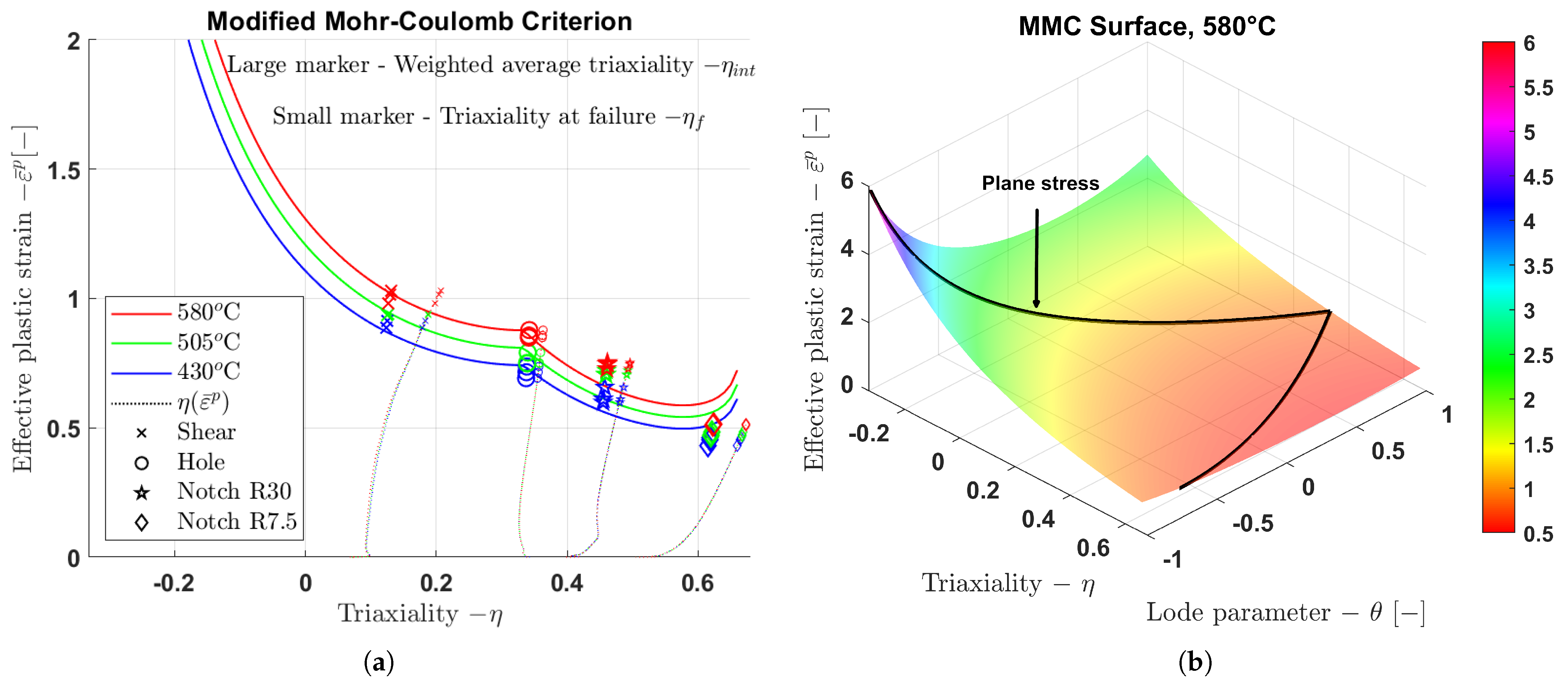
2.4. Calibration of Fracture Criterion
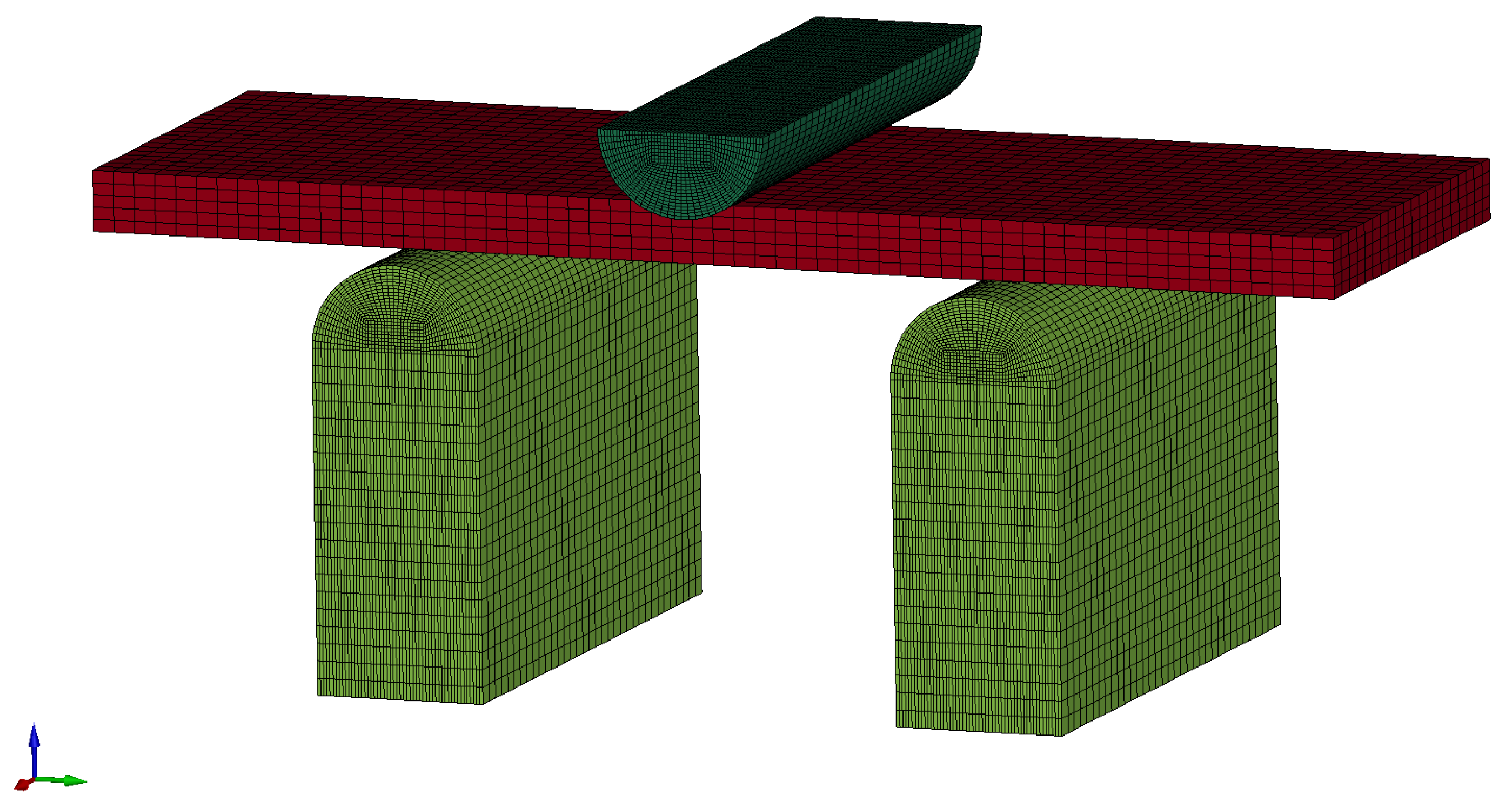
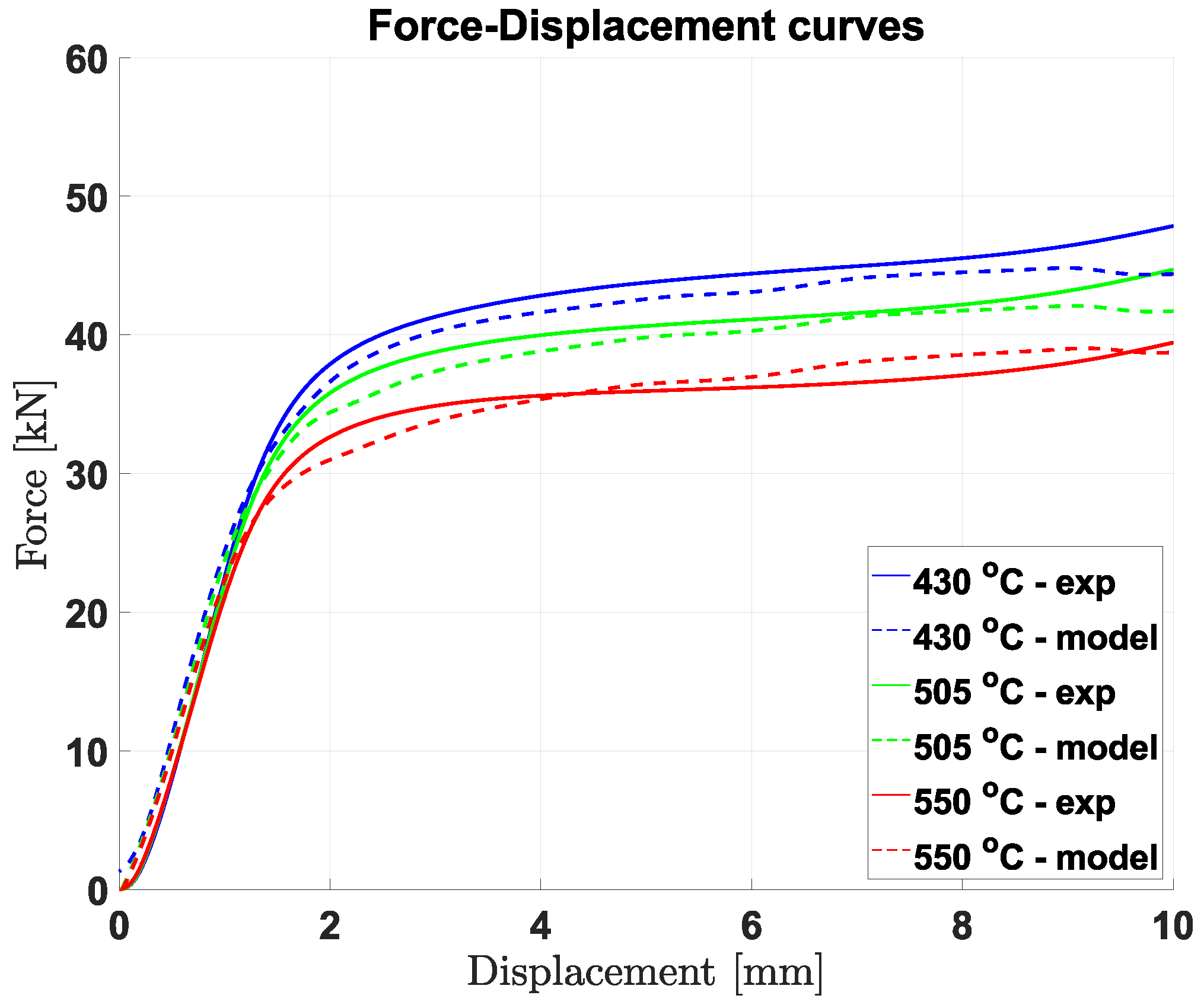
2.5. Validation by Three-Point Bending
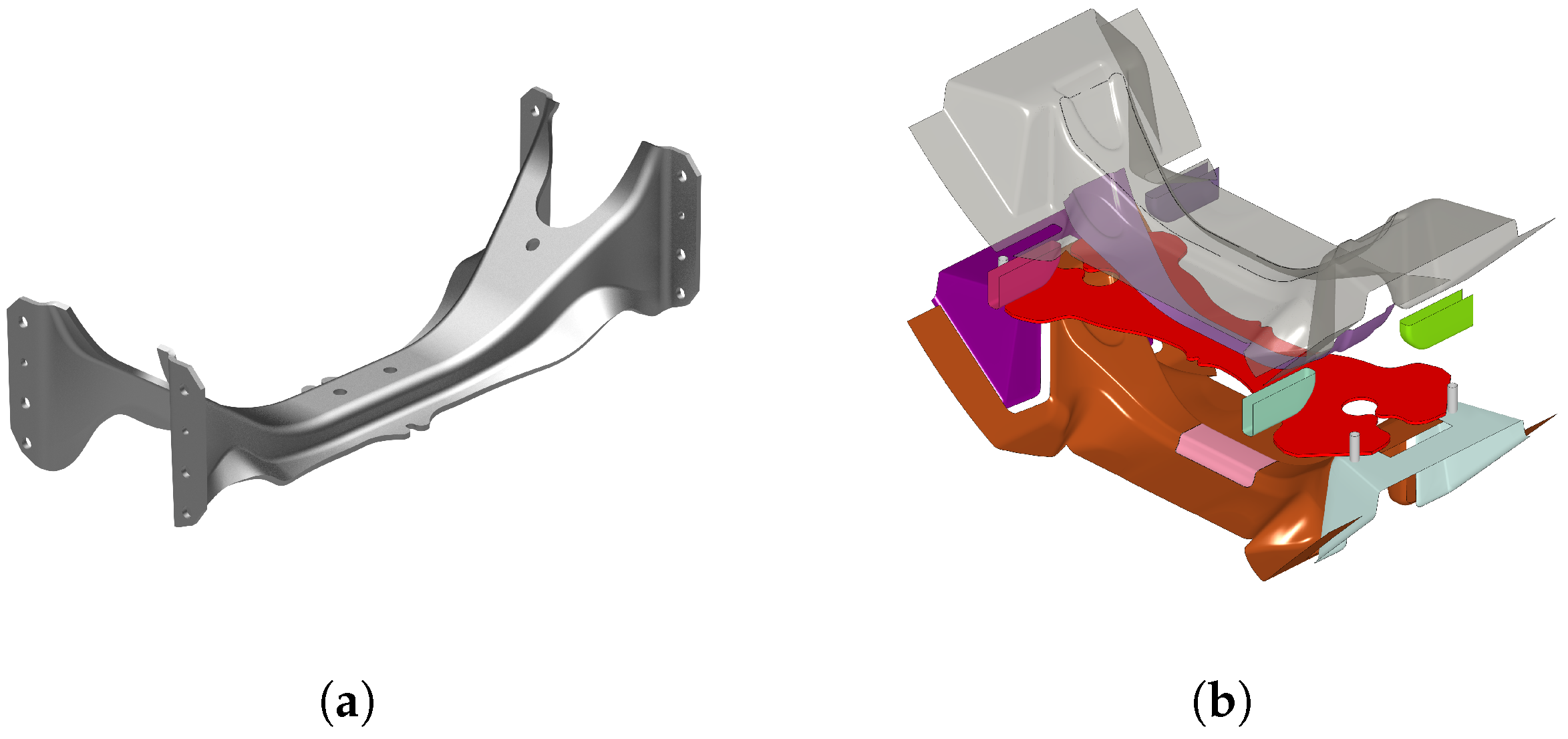
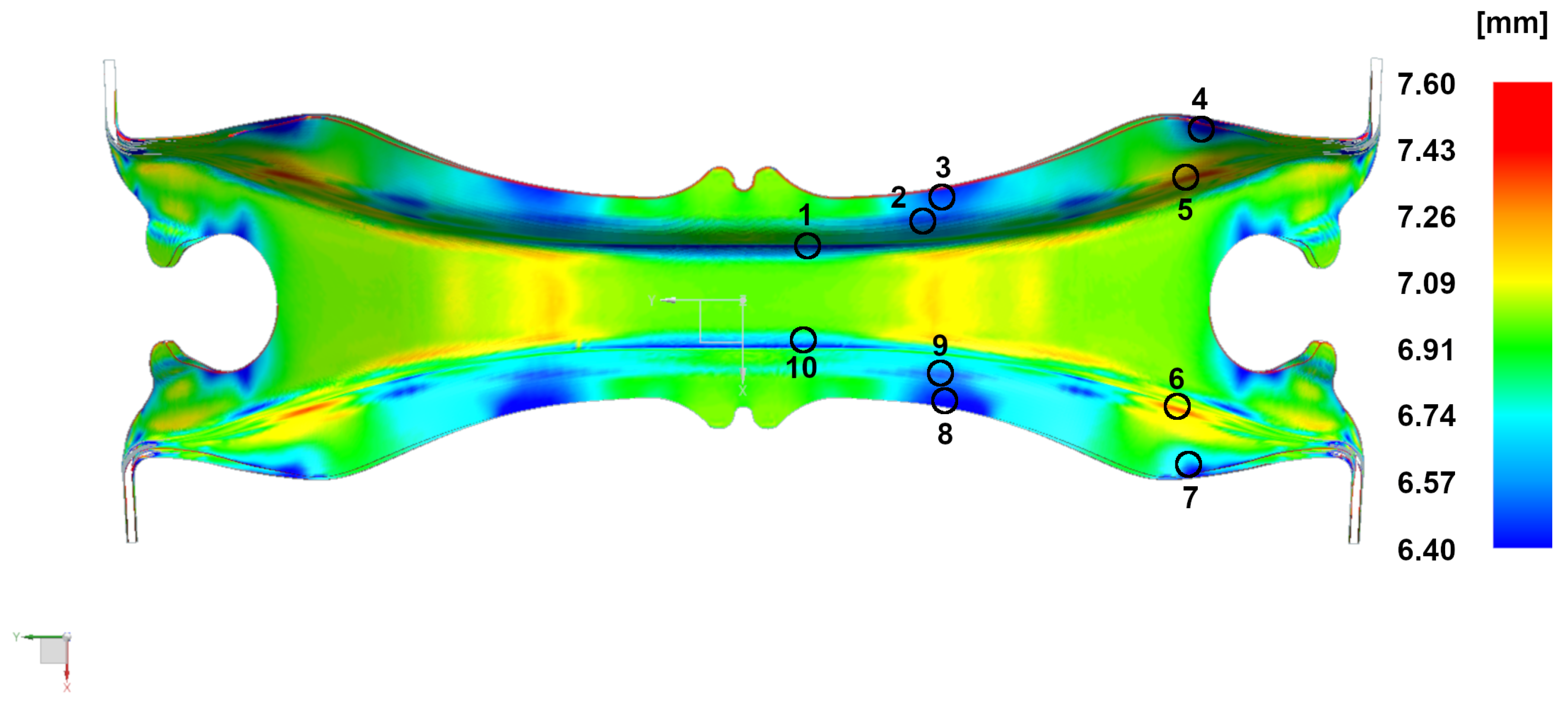
2.6. Validation by Forming of an HDV Chassis Crossmember
3. Results
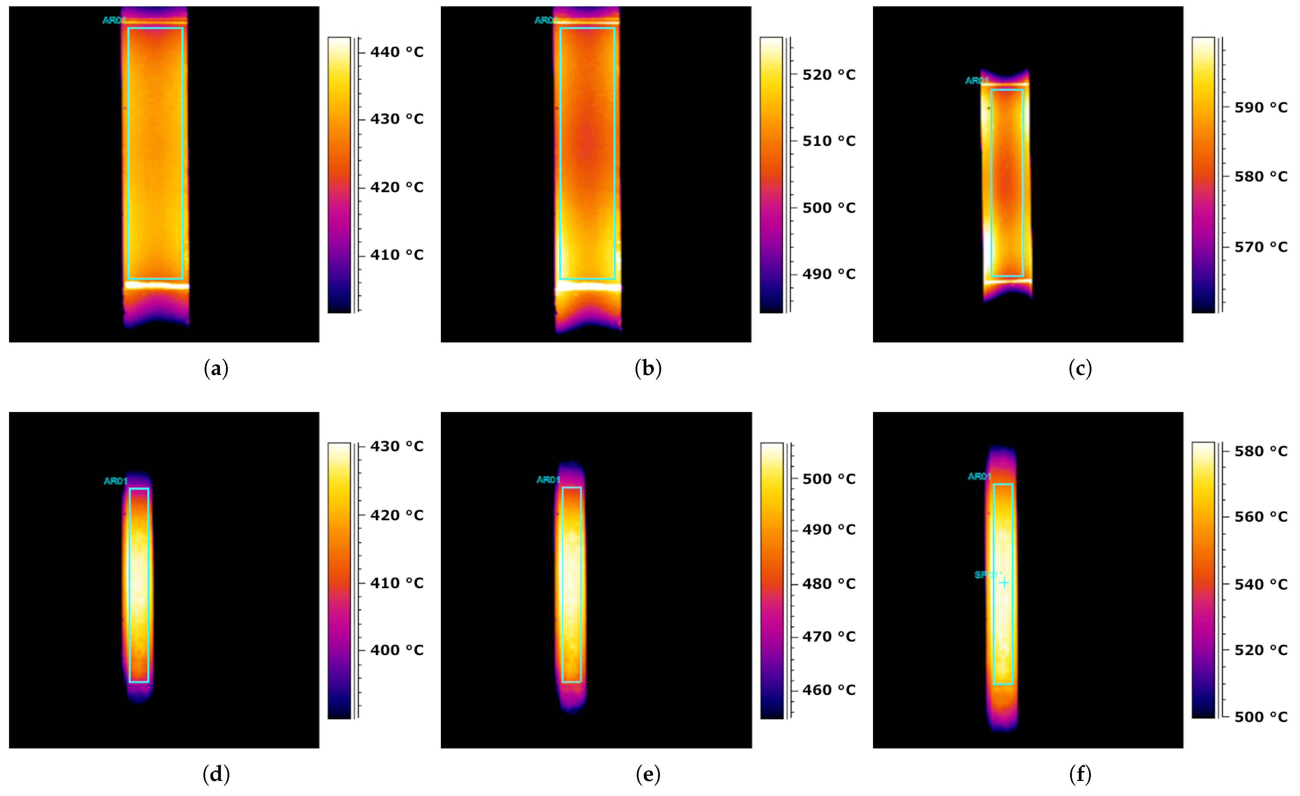
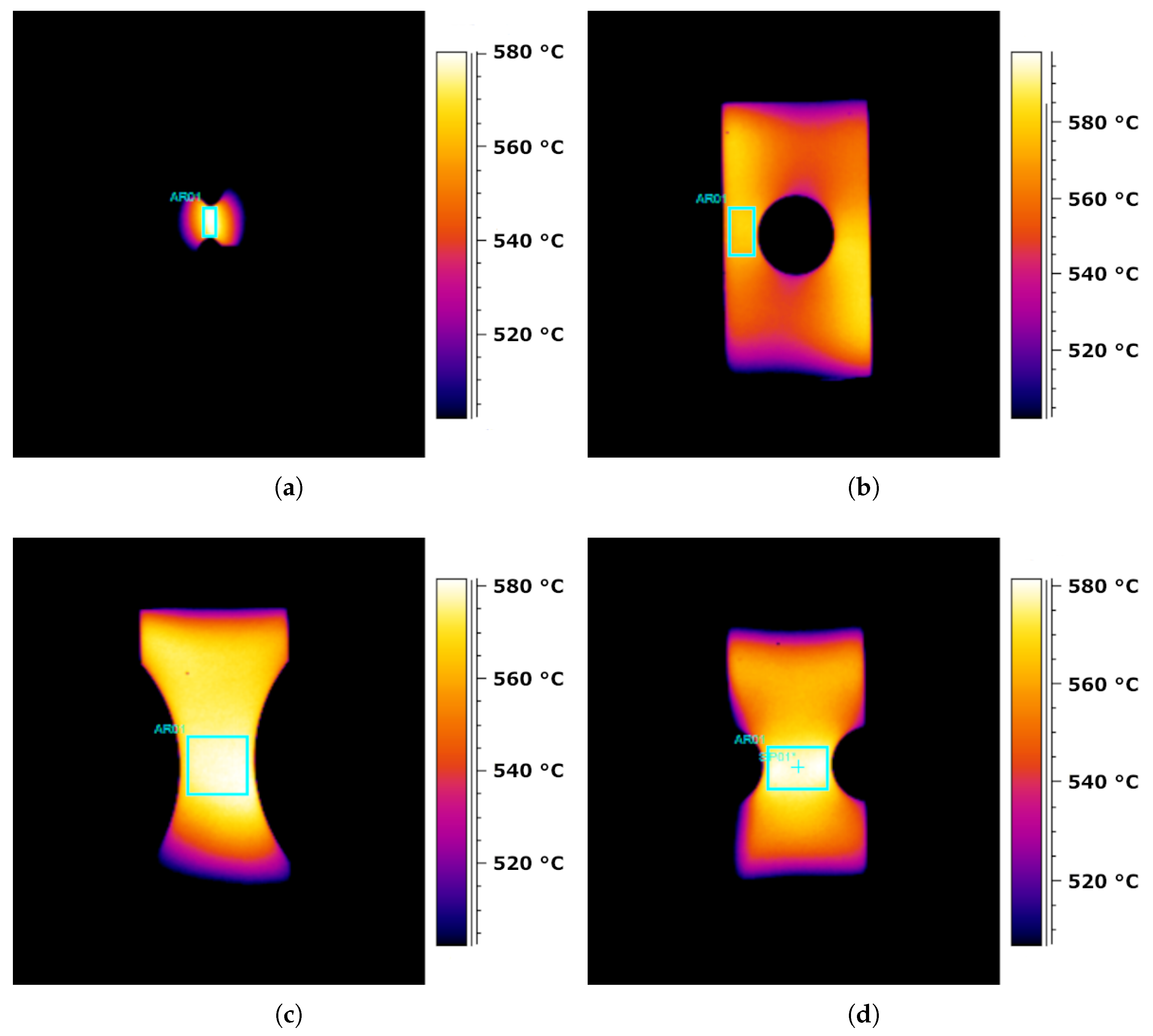
3.1. Heat Distribution
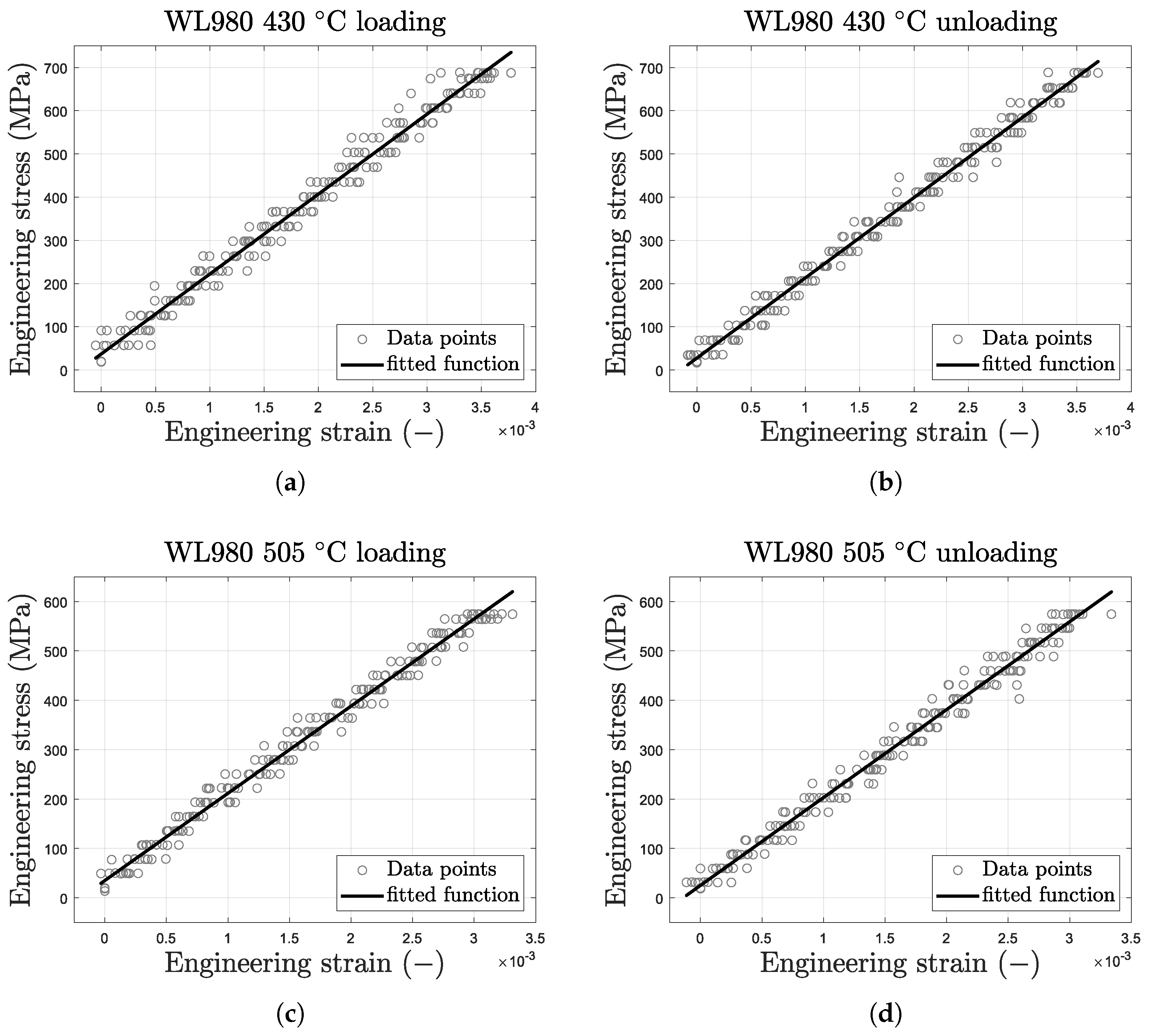
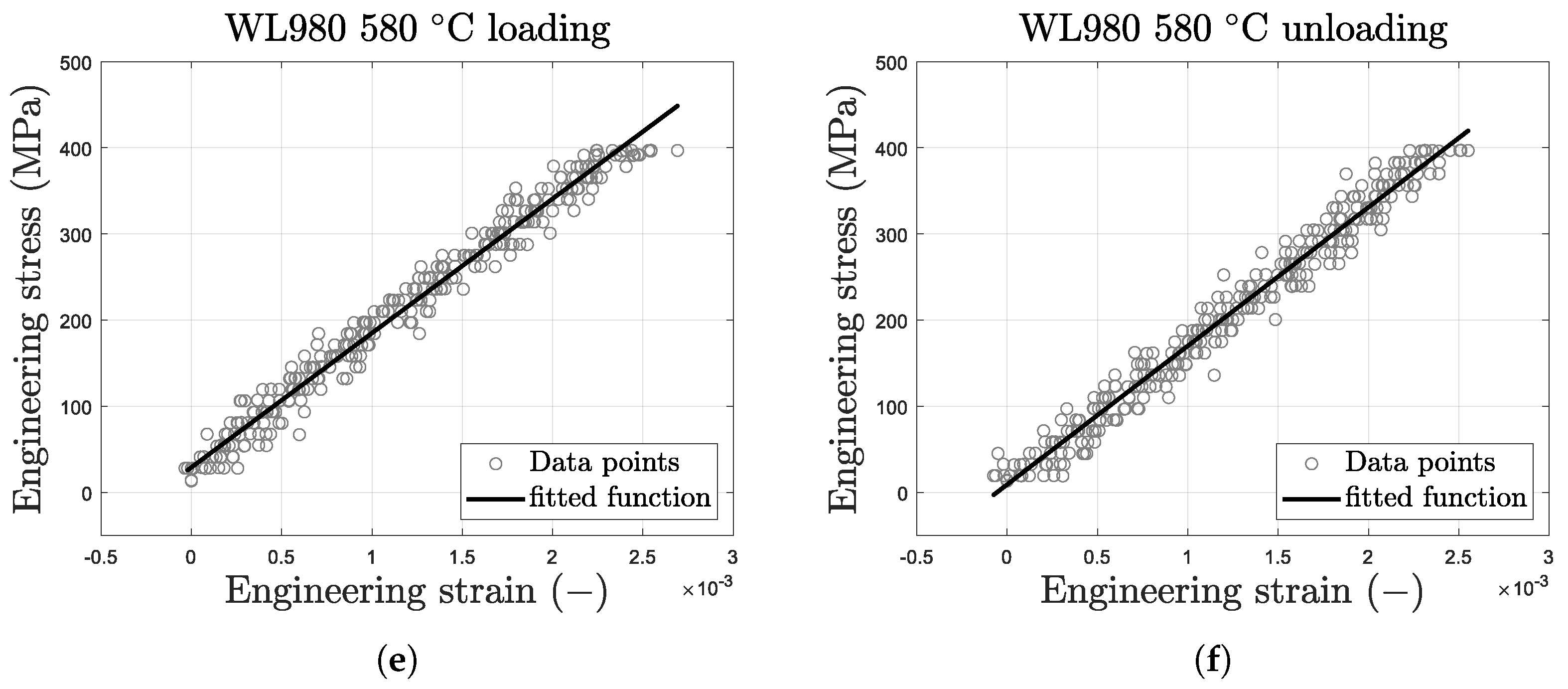
3.2. Young’s Modulus
3.3. Calibration of Temperature-Dependent Work-Hardening Model
3.4. Calibration of Fracture Criterion
3.5. Three-Point Bending Validation
3.6. Thinning Comparison: Model vs. Prototype Crossmember
4. Discussion and Conclusions
Author Contributions
Funding
Data Availability Statement
Acknowledgments
Conflicts of Interest
Abbreviations
| AHSS | Advanced high-strength steel |
| BiW | Body-in-white |
| CAE | Computer-aided engineering |
| DIC | Digital image correlation |
| EDM | Electrical discharge machining |
| EV | Electric vehicle |
| GHG | Greenhouse gas |
| GISSMO | Generalised Incremental Stress-State-Dependent Damage Model |
| HDV | Heavy-duty vehicle |
| hists | Histories |
| HJP | Hollomon–Jaffe parameter |
| HP | Tempering parameter |
| HSS | High-strength steel |
| MMC | Modified Mohr–Coulomb |
| pars | Parameters |
| PHS | Press-hardened steel |
| resp | Responses |
| SEM | Scanning electron microscopy |
| SLR | Simple linear regression |
| UHSS | Ultra high-strength steel |
| UTS | Ultimate tensile strength |
| var | Variable |
References
- European Commission. WHITE PAPER, Roadmap to a Single European Transport Area—Towards a Competitive and Resource Efficient Transport System; Technical Report; European Commission: Brussels, Belgium, 2011. [Google Scholar]
- Hill, N.; Finnegan, S.; Norris, J.; Brannigan, C.; Wynn, D.; Baker, H.; Skinner, I. Reduction and Testing of Greenhouse Gas (GHG) Emissions from Heavy Duty Vehicles—Lot 1: Strategy; Technical Report; European Commission: Brussels, Belgium, 2011. [Google Scholar]
- Mulholland, E.; Teter, J.; Cazzola, P.; McDonald, Z.; Gallachóir, B.P.Ó. The long haul towards decarbonising road freight—A global assessment to 2050. Appl. Energy 2018, 216, 678–693. [Google Scholar] [CrossRef]
- Heywood, J.; MacKenzie, D.; Akerlind, I.B.; Bastani, P.; Berry, I.; Bhatt, K.; Chao, A.; Chow, E.; Karplus, V.; Keith, D.; et al. On the Road Toward 2050: Potential for Substantial Reductions in Light-Duty Vehicle Energy Use and Greenhouse Gas Emissions; Massachusetts Institute of Technology: Cambridge, MA, USA, 2015; p. 286. [Google Scholar]
- Tisza, M.; Lukács, Z. High strength aluminum alloys in car manufacturing. In Proceedings of the IOP Conference Series: Materials Science and Engineering, Waterloo, ON, Canada, 3–7 June 2018; IOP Publishing: Bristol, UK, 2018; Volume 418. [Google Scholar] [CrossRef]
- Tokita, Y.; Nakagaito, T.; Tamai, Y.; Urabe, T. Stretch formability of high strength steel sheets in warm forming. J. Mater. Process. Technol. 2017, 246, 77–84. [Google Scholar] [CrossRef]
- Karbasian, H.; Tekkaya, A.E. A review on hot stamping. J. Mater. Process. Technol. 2010, 210, 2103–2118. [Google Scholar] [CrossRef]
- Marquis, G.; Barsoum, Z. Fatigue strength improvement of steel structures by high-frequency mechanical impact: Proposed procedures and quality assurance guidelines. Weld. World 2014, 58, 19–28. [Google Scholar] [CrossRef]
- Parareda, S.; Casellas, D.; Frómeta, D.; Grifé, L.; Lara, A.; Pujante, J.; Hackl, R.; Sonnleitner, M.; Sieurin, H. Warm Forming of Hot Rolled High Strength Steels-with Enhanced Fatigue Resistance as a Lightweight Solution for Heavy Duty Vehicles. In Proceedings of the 8th International Conference Hot Sheet Metal Forming of High-Performance Steel (CHS2 2022), Barcelona, Spain, 30 May–2 June 2022. [Google Scholar]
- Prakash, V.; Ravi Kumar, D. Numerical analysis of non-isothermal warm deep drawing of an Al-Mg alloy using different yield criteria and experimental validation. Proc. Inst. Mech. Eng. Part E J. Process Mech. Eng. 2024, 238, 585–594. [Google Scholar] [CrossRef]
- Shrivastava, A.; Digavalli, R.K. Effect of Process Variables on Interface Friction Characteristics in Strip Drawing of AA 5182 Alloy and Its Formability in Warm Deep Drawing. J. Manuf. Mater. Process. 2023, 7, 175. [Google Scholar] [CrossRef]
- Saito, N.; Fukahori, M.; Hisano, D.; Hamasaki, H.; Yoshida, F. Effects of temperature, forming speed and stress relaxation on springback in warm forming of high strength steel sheet. Procedia Eng. 2017, 207, 2394–2398. [Google Scholar] [CrossRef]
- Sun, Y.; Wang, K.; Politis, D.J.; Chen, G.; Wang, L. An experimental investigation on the ductility and post-form strength of a martensitic steel in a novel warm stamping process. J. Mater. Process. Technol. 2020, 275, 116387. [Google Scholar] [CrossRef]
- Pandre, S.; Morchhale, A.; Kotkunde, N.; Singh, S.K.; Ravindran, S. Prediction of forming limits and microstructural evolution during warm stretch forming of DP590 steel. Arch. Civ. Mech. Eng. 2021, 21, 108. [Google Scholar] [CrossRef]
- Bao, Y.; Wierzbicki, T. On fracture locus in the equivalent strain and stress triaxiality space. Int. J. Mech. Sci. 2004, 46, 81–98. [Google Scholar] [CrossRef]
- Jonsson, S.; Kajberg, J. Evaluation of Crashworthiness Using High-Speed Imaging, 3D Digital Image Correlation, and Finite Element Analysis. Metals 2023, 13, 1834. [Google Scholar] [CrossRef]
- Sjöberg, T.; Kajberg, J.; Oldenburg, M. Fracture behaviour of Alloy 718 at high strain rates, elevated temperatures, and various stress triaxialities. Eng. Fract. Mech. 2017, 178, 231–242. [Google Scholar] [CrossRef]
- Schill, M.; Zhu, X. Simulation of Sheet Metal Forming Using Solid Elements Using ANSYS LS-DYNA ©. In Proceedings of the 2024 International LS-DYNA Conference, Metro Detroit, MI, USA, 22–23 October 2024. [Google Scholar]
- Grange, R.A.; Hribal, C.R.; Porter, L.F. Hardness of Tempered Martensite in Carbon and Low-Alloy Steels. Metall. Trans. A 1977, 8, 1775–1785. [Google Scholar] [CrossRef]
- Hollomon, J.H.; Jaffe, L.D. Time-temperature Relations in Tempering Steel—Technical Publication No. 1831. Met. Technol. 1945, 11, 1–26. [Google Scholar]
- Tsuchiyama, T. Physical Meaning of Tempering Parameter and Its Application for Continuous Heating or Cooling Heat Treatment Process. J. Jpn. Soc. Heat Treat. 2002, 42, 163–168. [Google Scholar]
- Revilla, C.; López, B.; Rodriguez-Ibabe, J.M. Carbide size refinement by controlling the heating rate during induction tempering in a low alloy steel. Mater. Des. 2014, 62, 296–304. [Google Scholar] [CrossRef]
- ISO 6892-1:2019; Metallic Materials—Tensile Testing—Part 1: Method of Test at Room Temperature. International Organization for Standardization: Geneva, Switzerland, 2019.
- Zou, K.H.; Tuncali, K.; Silverman, S.G. Correlation and simple linear regression. Radiology 2003, 227, 617–628. [Google Scholar] [CrossRef]
- Ilg, C.; Haufe, A.; Koch, D.; Stander, N.; Witowski, K.; Svedin, Å.; Liewald, M. Application of a Full-Field Calibration Concept for Parameter Identification of HS-Steel with LS-OPT®. In Proceedings of the 15th International LS-DYNA® Users Conference, Dearborn, MI, USA, 10–12 June 2018. [Google Scholar]
- Gorji, M.B.; Furmanski, J.; Mohr, D. From macro- to micro-experiments: Specimen-size independent identification of plasticity and fracture properties. Int. J. Mech. Sci. 2021, 199, 106389. [Google Scholar] [CrossRef]
- El-Magd, E.; Treppman, C.; Korthäuer, M. Description of flow curves over wide ranges of strain rate and temperature. Int. J. Mater. Res. 2006, 97, 1453–1459. [Google Scholar] [CrossRef]
- Mecking, H.; Kocks, U. Kinetics of flow and strain-hardening. Acta Metall. 1981, 29, 1865–1875. [Google Scholar] [CrossRef]
- Johnson, G.R.; Cook, W.H. Fracture characteristics of three metals subjected to various strains, strain rates, temperatures and pressures. Eng. Fract. Mech. 1985, 21, 31–48. [Google Scholar] [CrossRef]
- Stander, N.; Basudhar, A.; Roux, W.; Liebold, K.; Trent Eggleston, D.M.; Goel, T.; Craig, K. LS-OPT® User’s Manual A Design Optimization And Probabilistic Analysis Tool for the Engineering Analyst; Livermore Software Technology: Livermore, CA, USA, 2020. [Google Scholar]
- Bai, Y.; Wierzbicki, T. Application of extended Mohr-Coulomb criterion to ductile fracture. Int. J. Fract. 2010, 161, 1–20. [Google Scholar] [CrossRef]
- Livermore Software Technology Corporation (LSTC). LS-DYNA Keyword User’s Manual Volume II: Material Models; Livermore Software Technology Corporation: Livermore, CA, USA, 2021. [Google Scholar]
- Livermore Software Technology Corporation (LSTC). LS-DYNA Keyword User’s Manual Volume I; Livermore Software Technology Corporation: Livermore, CA, USA, 2021. [Google Scholar]
- Chen, J.; Young, B.; Asce, M.; Uy, B. Behavior of High Strength Structural Steel at Elevated Temperatures. J. Struct. Eng. 2006, 132, 1948–1954. [Google Scholar] [CrossRef]

| C | Si | Mn | Al | Cr | Ni + Mo | V + Nb | Ti | B |
|---|---|---|---|---|---|---|---|---|
| 0.09 | 0.10 | 1.6 | 0.05 | 0.9 | 0.7 | 0.1 | 0.02 | 0.0025 |
| Temperature (°C) | 7 mm—Average Yield Stress (MPa) | 7 mm—Average Peak Stress (MPa) | 1.2 mm—Average Peak Stress (MPa) | Percentage Change (%) |
|---|---|---|---|---|
| 430 | 824 ± 3 | 895 ± 1 | 882 ± 4 | −1.45 |
| 505 | 755 ± 1 | 809 ± 3 | 801 ± 5 | −0.97 |
| 580 | 607 ± 5 | 652 ± 6 | 651 ± 7 | −0.16 |
| Thickness (mm) | Target Temperature (°C) | Average Temperature (°C) | Temperature Span (°C) | Standard Deviation |
|---|---|---|---|---|
| 1.2 | 430 | 431 | 19 | 2.8 |
| 1.2 | 505 | 511 | 23 | 4.4 |
| 1.2 | 580 | 587 | 24 | 3.9 |
| 7 | 430 | 422 | 30 | 7.3 |
| 7 | 505 | 498 | 31 | 7.1 |
| 7 | 580 | 574 | 35 | 7.4 |
| Specimen Type | Target Temperature (°C) | Average Temperature (°C) | Temperature Span (°C) | Standard Deviation |
|---|---|---|---|---|
| Shear (a) | 580 | 579 | 11 | 1.7 |
| Hole (b) | 580 | 578 | 11 | 1.8 |
| R30 (c) | 580 | 579 | 12 | 2.4 |
| R7.5 (d) | 580 | 577 | 12 | 3.0 |
| Temperature (°C) | Loading | Unloading | Average Young’s Modulus (GPa) | ||
|---|---|---|---|---|---|
| Young’s Modulus (GPa) | Goodness of Fit, | Young’s Modulus (GPa) | Goodness of Fit, | ||
| 430 | 185 | 0.984 | 186 | 0.989 | 185 |
| 505 | 177 | 0.988 | 178 | 0.985 | 177 |
| 580 | 156 | 0.978 | 161 | 0.975 | 159 |
| C1 [MPa] | C2 [MPa] | C3 [MPa] | C4 | D | m |
|---|---|---|---|---|---|
| 824 | 205 | 59 | 363 | 6.82 | 1.65 |
| n | d | ||
|---|---|---|---|
| 0.352 | 1.58 | 0.358 | 1.30 |
| Point | 1 | 2 | 3 | 4 | 5 | 6 | 7 | 8 | 9 | 10 |
|---|---|---|---|---|---|---|---|---|---|---|
| 3D Scanning [mm] | 5.88 | 6.56 | 6.55 | 6.34 | 7.40 | 7.33 | 6.53 | 6.44 | 6.51 | 5.94 |
| Model [mm] | 6.41 | 6.52 | 6.50 | 6.36 | 7.37 | 7.32 | 6.50 | 6.41 | 6.50 | 6.37 |
| Percentage difference [%] | 8.63 | 0.61 | 0.77 | 0.32 | 0.41 | 0.14 | 0.46 | 0.47 | 0.15 | 6.99 |
Disclaimer/Publisher’s Note: The statements, opinions and data contained in all publications are solely those of the individual author(s) and contributor(s) and not of MDPI and/or the editor(s). MDPI and/or the editor(s) disclaim responsibility for any injury to people or property resulting from any ideas, methods, instructions or products referred to in the content. |
© 2025 by the authors. Licensee MDPI, Basel, Switzerland. This article is an open access article distributed under the terms and conditions of the Creative Commons Attribution (CC BY) license (https://creativecommons.org/licenses/by/4.0/).
Share and Cite
Larsson, F.; Hammarberg, S.; Jonsson, S.; Kajberg, J. Material Characterisation, Modelling, and Validation of a UHSS Warm-Forming Process for a Heavy-Duty Vehicle Chassis Component. Metals 2025, 15, 424. https://doi.org/10.3390/met15040424
Larsson F, Hammarberg S, Jonsson S, Kajberg J. Material Characterisation, Modelling, and Validation of a UHSS Warm-Forming Process for a Heavy-Duty Vehicle Chassis Component. Metals. 2025; 15(4):424. https://doi.org/10.3390/met15040424
Chicago/Turabian StyleLarsson, Fredrik, Samuel Hammarberg, Simon Jonsson, and Jörgen Kajberg. 2025. "Material Characterisation, Modelling, and Validation of a UHSS Warm-Forming Process for a Heavy-Duty Vehicle Chassis Component" Metals 15, no. 4: 424. https://doi.org/10.3390/met15040424
APA StyleLarsson, F., Hammarberg, S., Jonsson, S., & Kajberg, J. (2025). Material Characterisation, Modelling, and Validation of a UHSS Warm-Forming Process for a Heavy-Duty Vehicle Chassis Component. Metals, 15(4), 424. https://doi.org/10.3390/met15040424