Carbon Steel A36 Planar Coupons Exposed to a Turbulent Flow Inside a 90° Pipe Elbow in a Testing Rack: Hydrodynamic Simulation and Corrosion Studies

Abstract

This work aims to characterize flow-accelerated corrosion of carbon steel A36 coupons exposed to simulated treated reverse-osmosis seawater under ambient conditions and a Reynolds number range of 6000 to 25,000 using a standard corrosion testing method. The flow behavior in the corrosion compartment and the turbulent parameters were determined by computational fluid dynamics simulation. Using selected flow parameters, complemented with experimental corrosion rate measurements, the oxygen mass transfer coefficients (m_c) and the rate constant for the cathodic reaction (k_c) at the coupon surface were determined. As expected, m_c depends only on the fluid conditions, while k_c is highly influenced by interface resistance, leading to significantly different runs with and without a corrosion inhibitor. The dissimilar fluid flow distribution on intrados and extrados generates irregular corrosion patterns, depending on the angular position of the coupon inside the corrosion compartment. Morphological studies using scanning electron microscopy and atomic force microscopy support simulation results.

1. Introduction

Using standard corrosion testing methods is of primary importance in industrial engineering because it helps assess and predict the durability of materials and components in various environments. There are many standard methods for testing steel to determine the corrosivity of water under flow accelerated corrosion (FAC) conditions inside pipes. One such method, referred to as ASTM D 2688-05, typically employs flat, rectangular-shaped metal coupons, which are mounted on pipe plugs and exposed to the water flowing through metal piping in municipal, building, and industrial water systems using a side-stream corrosion specimen rack [1].

FAC is essentially a slow metal degradation process caused by fluid flow removing the protective oxide layers from piping components. It involves a combination of electrochemical reactions, erosion of the oxide layer on carbon steel pipe walls, and mass transfer to the flow, all of which are accelerated by the hydrodynamics of the fluid flow within the piping system. Factors such as the geometrical configuration and orientation of the piping component, fluid temperature, and piping material can significantly affect FAC [2,3,4,5].

Elemuren et al. [6] examined the influence of flow velocities on erosion–corrosion in a 90° carbon steel elbow in potash brine at 30 °C. The metal specimens were bends installed in a closed-loop polyvinylchloride (PVC) tubing system, circulating fluid at velocities between 2.5 and 4 m s⁻¹. Experimental monitoring consisted of weight loss measurements of the bends together with morphological characterization. The main conclusion was that at low velocities, degradation was dominated by corrosion attack, as evidenced by the presence of corrosion pits on the elbow surface. In contrast, erosive wear was the dominant damage mechanism at high slurry velocities.

Slaimana and Hasan [7] have studied the effect of corrosion products on the corrosion rate of carbon steel pipe in aerated 0.1 N NaCl solution under turbulent flow. Tests were conducted using the electrochemical polarization technique to determine the limiting current density of oxygen reduction over a Reynolds number (Re) range of 15,000 to 113,000 and a temperature range of 30–60 °C. Their main conclusion was that the formation of corrosion products over time decreases the corrosion rate at low Re and temperature, while it increases the corrosion rate at high Re and temperature.

Si et al. [8] have investigated the effects of turbulent parameters on the FAC of low-carbon steel at the 90° elbow through experiments and numerical simulation. An array of electrodes was used for electrochemical measurements of FAC at distinct locations of the 90° elbow. The experimental results showed that the maximum corrosion current density occurred on the extrados side of the test section, while the minimum value appears at the intrados side of the elbow. These findings are consistent with the typical FAC-induced failures observed in turbine plant pipelines and equipment.

Moon et al. [9] studied the hydrodynamic parameters influencing FAC in elbow sections to identify the locations highly susceptible to FAC. The results revealed that the side of the elbow pipe was the most susceptible to FAC because it experienced the most severe wall thinning. It was found that a combination of velocity and vorticity components was responsible for this behavior. Therefore, a combination of velocity and vorticity components should be used as hydrodynamic parameters to characterize FAC-induced wall thinning.

The present paper aims to characterize, both experimentally and numerically, the hydrodynamic effects of reverse-osmosis-treated seawater flow on flow-accelerated corrosion in a planar coupon positioned inside a 90° elbow using a standard corrosion testing method. The specific objectives are (i) to experimentally quantify the corrosion rate and the surface morphology of the coupon, compared to a coupon protected with a corrosion inhibitor, as affected by fluid velocity, and (ii) to numerically simulate and characterize the flow structures within the bend that influence corrosion distribution on the coupon. The experiments and simulations were performed for a 17 mm internal diameter abrupt bend at a maximum Reynolds number of 25,000. This research demonstrates the relevance of the CFD as a tool to improve the assessment and accuracy of experimental corrosion measurements in detecting sensitive zone locations exposed to flow accelerated corrosion and the effectiveness of the standard testing method.

2. Materials and Methods

2.1. Coupons and Reverse Osmosis Solutions

Rectangular coupons made of ASTM A36 carbon steel, with a nominal chemical composition of (%wt.): 0.27 C, 1.03 Mn, 0.2 Cu, 98 Fe, 0.04 P, 0.28 Si, 0.05 S, were used in all experiments. The coupons, with dimensions of 75 × 15 × 3 mm, were abraded sequentially using 600- to 1200-grit SiC emery paper, sonicated in ethylic alcohol, washed with acetone, dried in hot air, and finally weighed using a precision balance with an accuracy of 0.0001 g. For each run, the coupons were installed in the testing rack for 48 h. After the corroding period, the coupons were removed from the pipe network and then sequentially cleaned in an ultrasound bath with a 2% ascorbic acid solution, washed with ethanol, rinsed with acetone, dried in a hot air flow, and finally weighed again.

The test solution was a simulated reverse osmosis (RO) water prepared from distilled water by dosing measured amounts of sodium chloride, sodium sulphate, sodium carbonate, sodium borate, and magnesium chloride to achieve the following solution composition: sodium, 480 mg L⁻¹; chloride, 630 mg L⁻¹; sulphate, 200 mg L⁻¹; boron, 2.5 mg L⁻¹; carbonate and bicarbonate, 30 mg L⁻¹; and magnesium, 50 mg L⁻¹. The final pH of the RO water was adjusted to 7.5 by adding a few drops of a 1 M sulfuric acid solution. The final measured conductivity of the RO water was 1800 µS cm⁻¹. All chemicals used were of analytical grade (Sigma-Aldrich, Darmstadt, Germany). For the corrosion protection studies, a polyphosphate commercial corrosion inhibitor was used in a proven optimal dose of 20 mg L⁻¹.

2.2. Experimental Apparatus

The corrosion testing rack, shown in Figure 1, was used to assess the corrosion rate of metal coupons under flow conditions. This rack contains two coupon chambers that consist of a PVC Tee with two sides glued to vertical inlet and horizontal outlet PVC tubing. The third side of the Tee was glutted to a threaded cylindrical female connector adapted for watertight, concentric insertion of the plastic holder−coupon assembly. The RO water solution was contained in a 100 L tank (A) and pumped in a closed-loop system, with flow controlled by adjusting the rotation speed of a 1 kW three-phase pump (B) using a frequency converter. A total of six experimental runs, three without inhibitors and three with inhibitors, were conducted at different fluid velocities, as shown in

Table 1. Run simulations. Re number refers to inlet’s vertically reduced section.

Run	Flow, L s−1	Inlet Diameter, mm	Final Diameter, mm	Flow Velocity, m s−1	Re
1	0.28	28	17	1.47	24,939
2	0.14	28	17	0.73	12,470
3	0.07	28	17	0.37	6235

. For each run, two coupons were placed inside the corrosion compartment in vertical and horizontal positions.

2.3. Fluid Flow Simulation Along the Coupon Compartment

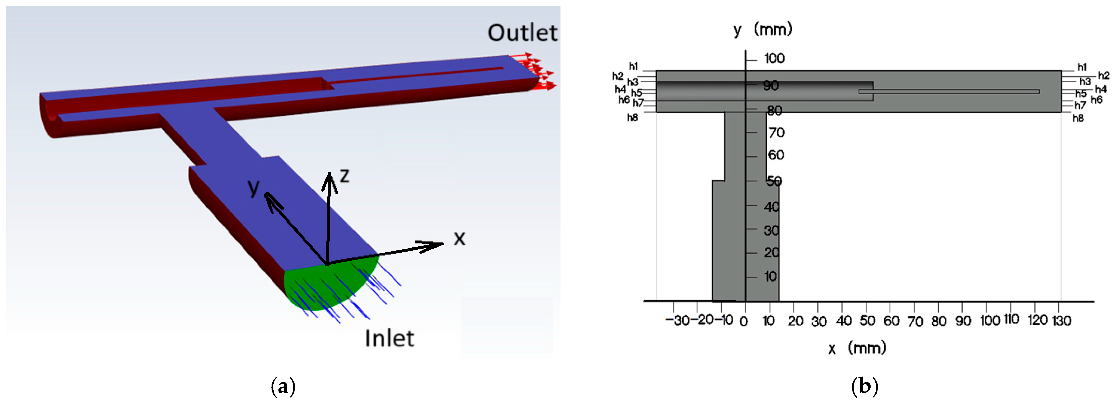
Computational fluid dynamic (CFD) simulation through the coupon compartment was performed using ANSYS Fluent software 2024 R2 [10] using a half-symmetric fluid volume model shown in Figure 2. The inlet section consisted of a PVC tube reducer from 28 to 17 mm in diameter, while the outlet PVC tube section maintained a constant diameter of 17 mm. The cylindrical and rectangular hollow sections at the outlet, shown in Figure 2, correspond to the holding fitting and coupon volumes, respectively.

Two main assumptions were adopted for the simulation: (a) a planar velocity profile at the inlet flow and (b) a symmetrical velocity distribution implied by the geometrical symmetry with respect to the x-y plane (Figure 3), allowing for a more accurate numerical solution.

The simulation was conducted under steady-state conditions, incorporating gravity and using a k-ω turbulent model. Under this model, the conservation laws for mass and momentum are averaged over a small-time increment, applying Reynold decomposition, where flow quantities are expressed in terms of a temporal mean and a fluctuating component. This fluctuating component is a function of the turbulent kinetic energy k (m² s⁻²), specific dissipation rate $\omega$ (s⁻¹), and eddy viscosity w (Pa s). Appendix A summarizes the basic conceptual framework for this model; a detailed description is found elsewhere [11,12]. Although the alternative RANS k-ɛ model has been extensively used in many erosion–corrosion situations [7,11,13,14], the standard k-ω model was selected in this work due to its better reported performance in the near-wall region compared to the k-ɛ model [14]. In addition, for the meshed geometry used in this study, a numerical convergence of 1 × 10^–5 in residuals for the main flow parameters was used. The more refined SST k-ω model produced almost identical results to the standard k-ω, although with higher convergence residual values.

The hydrodynamic simulation included three different conditions to match experimental runs (Table 1). The Re number is defined as $Re={\displaystyle \frac{\rho ·v·D}{\mu }}$, where $v$ is the flow velocity magnitude at the final diameter D of 17 mm, and $\rho$ and $\mu$ are the density and viscosity of the test solution, respectively.

For each flow condition, two coupons’ orientations were considered: one with the coupon in a horizontal position and one in a vertical position.

A half-symmetric fluid volume inside the corrosion compartment, showing the inlet and outlet ports and holding a coupon in a horizontal position, is shown in Figure 2.

From a 3D CAD drawing built to replicate the fluid volume with created surface regions for the inlet, outlet, symmetry plane, coupon surface, and walls, depicted in Figure 2, a mesh partitioning module was automatically generated, with mesh points clustered densely near the wall with three boundary layers. The total number of the polyhedral cells was 220,000, with sizes ranging between 0.1 and 0.6 mm. Using built-in tools of the Ansys Fluent 2024 R2 software, the mesh quality was evaluated satisfactorily with respect to orthogonal, skewness, and aspect ratio for the entire domain.

The boundary conditions considered were no-slip conditions under null rugosity for both coupon and internal walls, and flow inlet expressed as mass flow.

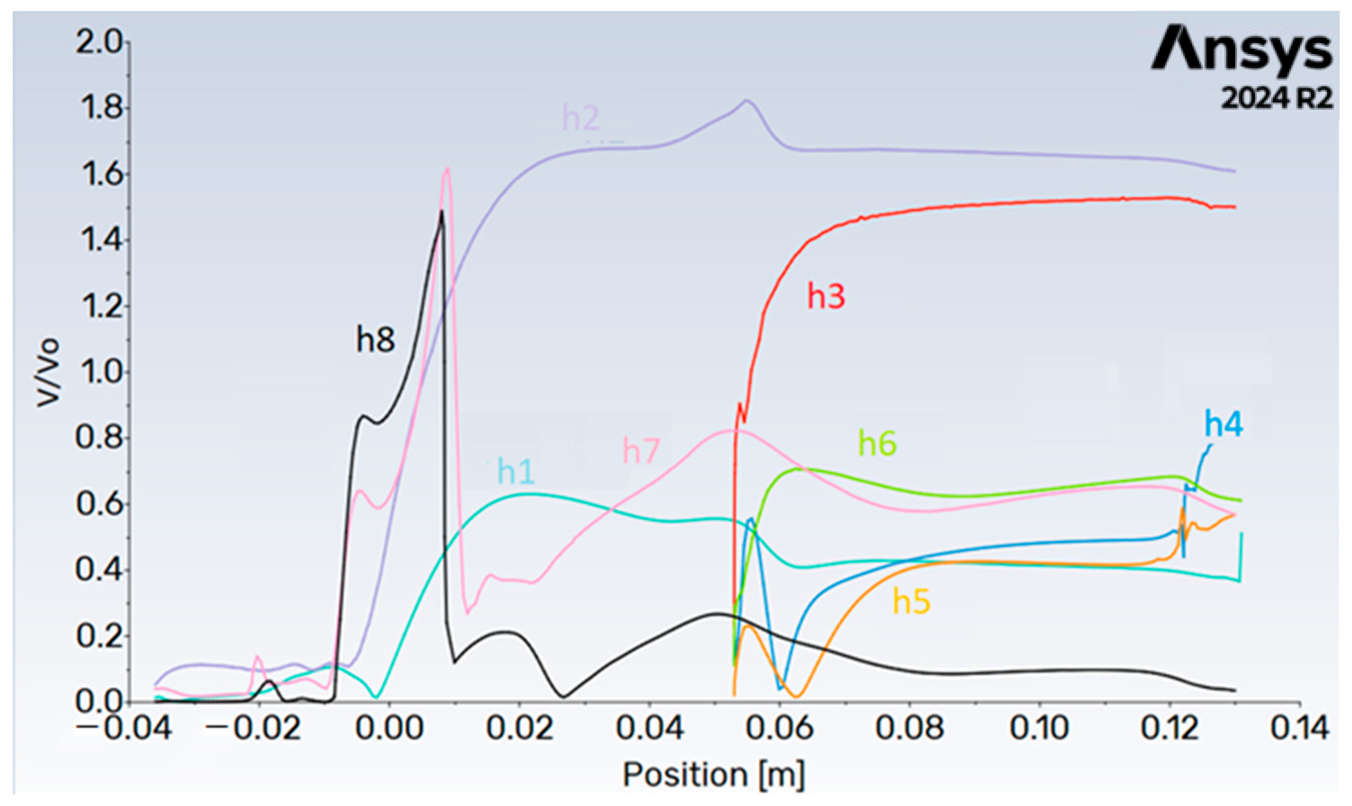
The simulation runs were made in a laptop Lenovo ThinkPad E16 de 2da Gen (16”, AMD) with no parallel processing; the processing time for each simulation was about 15 min. The convergence was achieved with a default solution method based on a coupled velocity–pressure scheme, with special discretization based on least square cell gradient for main flow parameters. The convergence was achieved after 300 runs approx., with a residual convergence for continuity equation and turbulent parameters adjusted to 10⁻⁵, two orders of magnitude lower than the maximum acceptable limit. It is important to mention that the default mesh size (1 to 5 mm)—suggested by the software—was reduced by one order of magnitude to minimize noise in velocity curves, thus obtaining smooth curves such as those of Figure 4. Once the simulation was finished, a task to process the results in chosen planes and curves was performed. For this purpose, lines and planes had to be created, taking in mind the zero-reference chosen when the CAD drawing was built (Figure 2).

2.4. Surface Analysis

Superficial characterization of coupons was carried out by scanning electron microscopy (SEM) using a Zeiss EVA MA 10 microscope (Zeiss company, Oberkochen, Germany) and by atomic force microscopy (AFM) using an Oxford-Jupiter XR instrument (Malvern Panalytical company, Malvern, Worcestershire, UK). The morphological patterns were analyzed in the absence and presence of inhibitor and by both sides of each coupon.

3. Results and Discussions

3.1. Hydrodynamic Simuations

3.1.1. Velocity Distribution and Vorticity

Figure 3 shows the normalized velocity profiles considering the local velocity ($v$) and the average velocity ($v_0$) and defined as $VN={\displaystyle \frac{\left|v\right|}{v_o}}$, in the 2D x-y plane. In general, the normalized flow velocity profile within the sharp bends is highly asymmetric and turbulent due to the interaction of two flow zones with different Reynolds numbers, one in the contraction vertical inlet and one after the abrupt 90° direction change. It is a reasonable assumption to consider that the angular position of the coupon with respect to its longitudinal x-axis will significantly alter the internal hydrodynamic pattern of the fluid flow, compared to a situation without the coupon. Accordingly, two angular positions of the coupon inside the corrosion compartment were considered: one horizontal and one vertical, as shown in Figure 3a and Figure 3b, respectively.

The contour plot velocity magnitude for simulated run 1, with the coupon positioned horizontally, is shown in Figure 3a. As flow passes through the concentric reducer, the average velocity increases from 0.89 to 1.47 m s⁻¹ for the inlet and the reduced section, respectively.

In the abrupt bending section shown in Figure 3a, it can be observed that the fluid velocity magnitude at the extrados is greater than at intrados. In fact, the red zones corresponding to higher velocities are seen only near the extrados in both axial and transverse c, d, and e zones. This observation is consistent with previous investigations [15,16,17]. The influence of the coupon’s angular position on the velocity distribution inside the corrosion compartment is noticeable in the flow direction inmediately after the coupon’s x-coordinate position, so that the normalized velocity values in cross-section views d and e for a vertically positioned coupon are significantly more homogeneous compared to those for a horizontally positioned coupon.

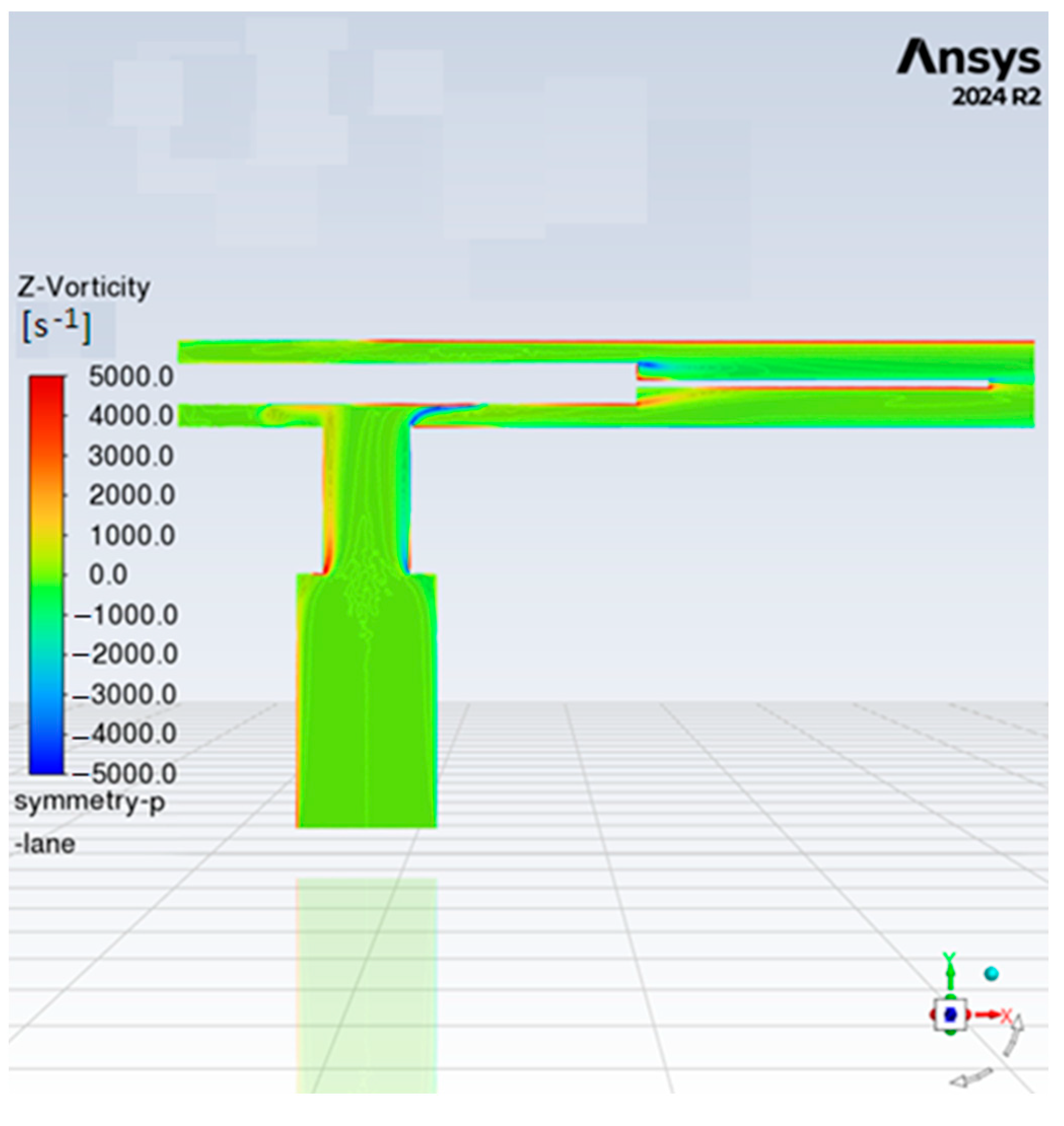
The velocity magnitude plot in Figure 4 shows irregular axial and traverse motion, with x and y velocity components that change directions near the abrupt bend and the coupon–plastic holder connection (Figure 5). These changes in x and y velocity components imply the occurrence of x-y vorticity, which can be characterized by a z-vorticity defined as ${\displaystyle \frac{\partial v_x}{\partial y}}-{\displaystyle \frac{\partial v_y}{\partial x}}$, as shown in Figure 6. The sign of the z-vorticity indicates the direction of rotation, either clockwise or counterclockwise, with both conditions observed in the reddish and blueish zones along the upper internal surface. Similarly, full 3D vorticity vector should take place with x, y, and z components and is defined as $\nabla \times v$. Its magnitude, $\left|\nabla \times v\right|$, referred to as the vorticity magnitude, is used in the formulation of the RANDS turbulence model (see Appendix A).

3.1.2. RANDS $k-\omega$ Parameters

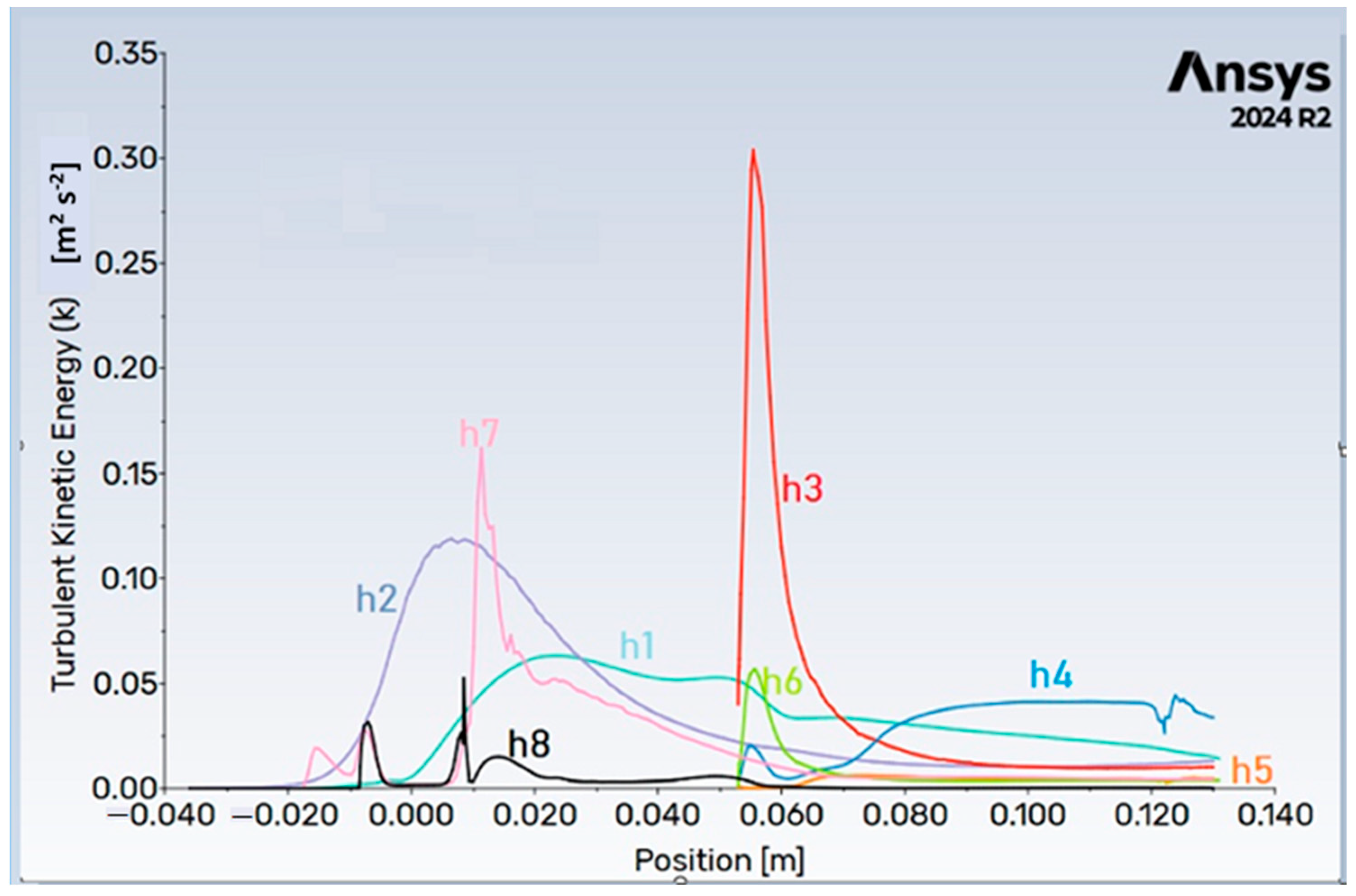
At VN values higher than 0.6 the fluctuating patterns observed in the symmetry plane (Figure 3) for both $k \mathrm{a}\mathrm{n}\mathrm{d} \omega$ parameters (Figure 7 and Figure 8) are very similar with those of fluid velocity, in contrast to the lower velocity fluctuations observed in the nearly quiescent zone on the left side. It is interesting to note that the profiles along walls h1 and h8 (pipe walls) and h4 and h5 (coupon walls) show significant differences in $k \mathrm{a}\mathrm{n}\mathrm{d} \omega$ values as compared to the lines h2 and h7, which passes through the fluid bulk. This suggests that, even at comparable velocities, energy dissipation occurs more intensely along the wall surface than within the bulk fluid.

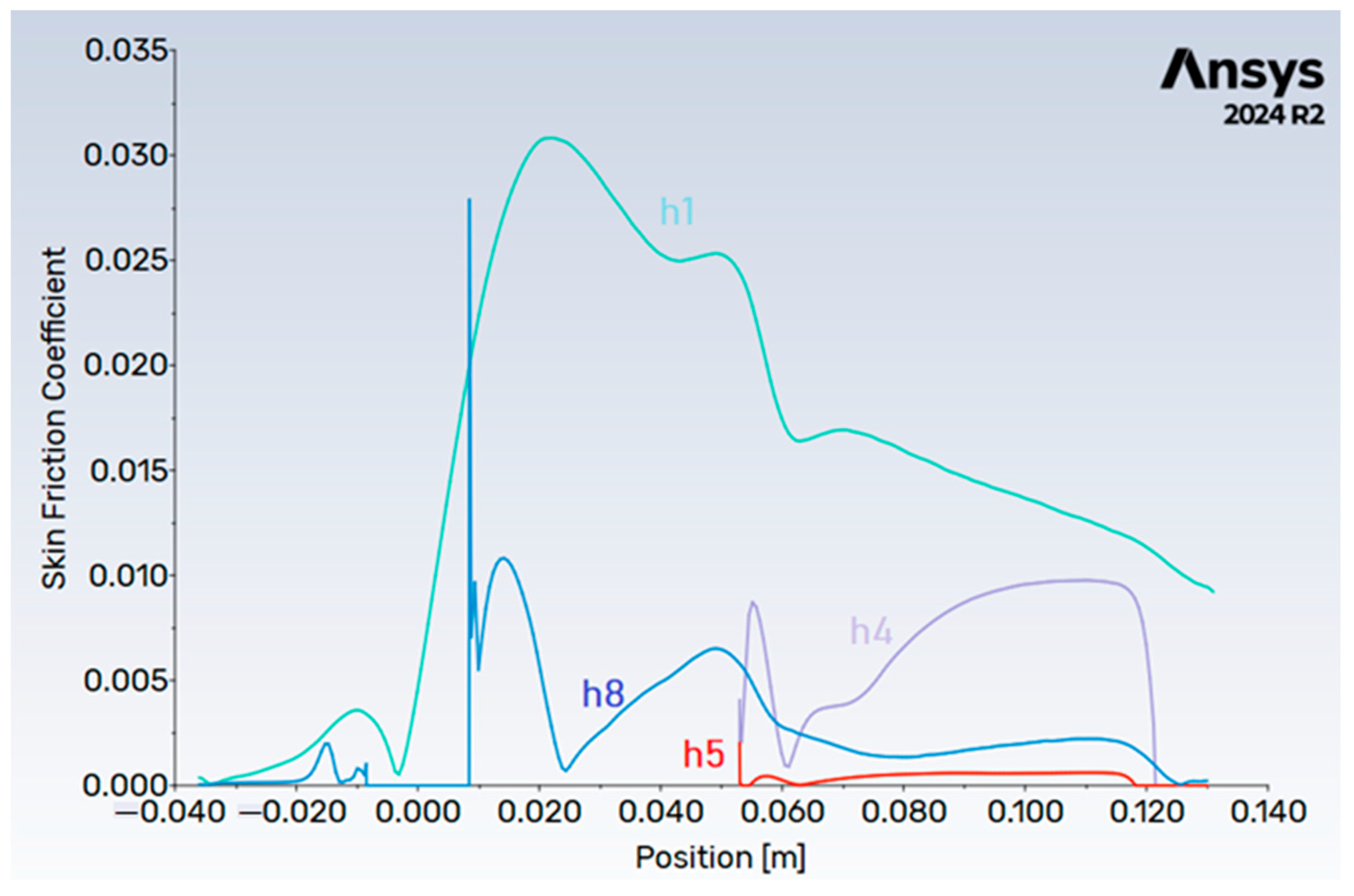
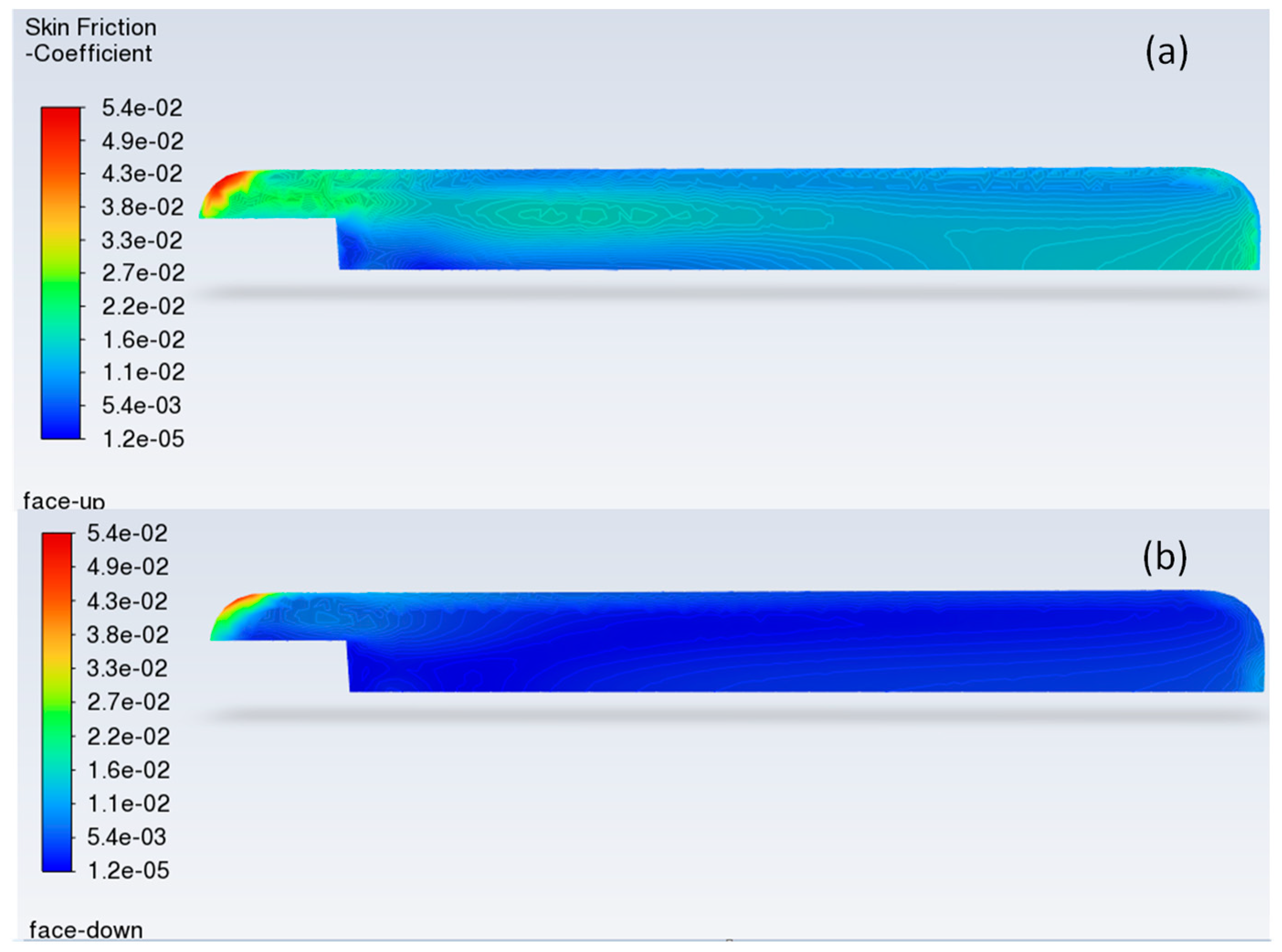
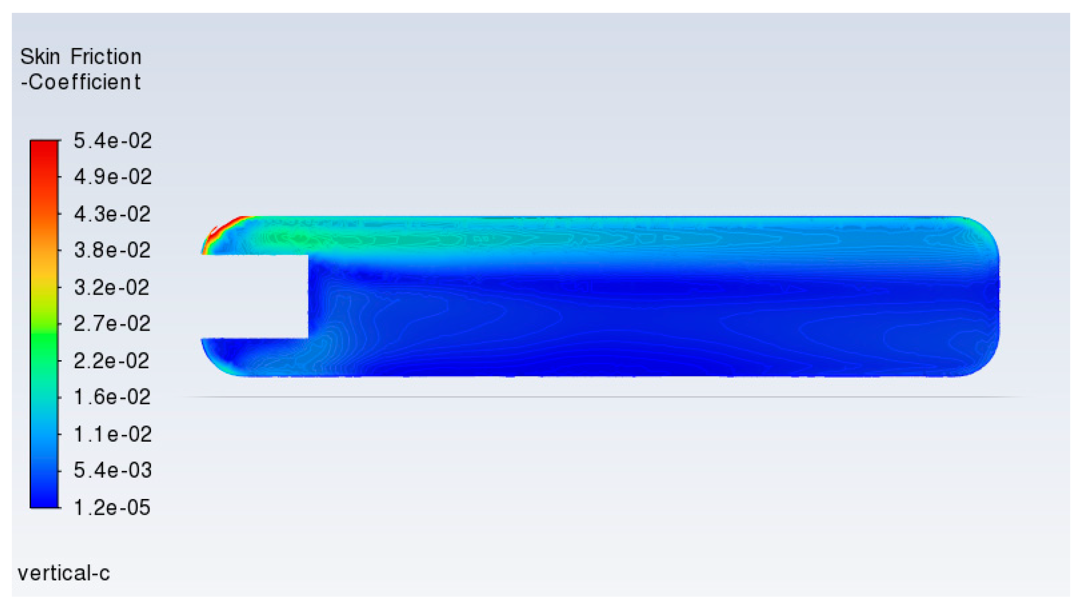
The skin friction coefficient ($f$) and wall shear stress along wall surfaces are important factors influencing the mass transfer coefficient in corrosion process and have been extensively studied in flow-accelerated corrosion scenarios [3,7]. Reported $f$ values at Re < 40,000 in these previous works [5,8] fall within the range of 0 to 0.0025, which match the values obtained for run 1 shown in Figure 9, Figure 10 and Figure 11. The highest $f$ values observed along the external tubing surface (line h1) are attributable to the greater fluid velocity magnitude at extrados circulation. This fluid distribution is also reflected as greater $f$ values in the face-up of the coupon (line h4) compared to the face-down side (line h5). The distribution of $f$ in the face-up and -down coupon surfaces is shown in Figure 10. The importance of this factor is further discussed in the next section.

Simulations for runs 2 and 3 with horizontal coupons and mass flow rates of 0.14 and 0.07 kg s⁻¹, respectively, show similar normalized velocity magnitudes and $f$ values compared to those observed in run 1 (0.28 kg s⁻¹). However, absolute velocity magnitudes, wall shear stress, and kinetic energy values vary in response to changes in the inlet velocity magnitude. Unlike the asymmetry in flow distribution observed between the face-up and face-down surfaces of the horizontal coupon (Figure 3 and Figure 10), the vertical coupons exhibit symetrical distributions (Figure 11).

3.1.3. Turbulence and Reynolds Number

In this section, for horizontal and vertical positioned coupons, three selected turbulence indicators versus Reynolds number are illustrated in

Table 2. Volume-averaged values over the fluid domain.

		Volume-Averaged Parameters
Re	Coupon Position	Vorticity Magnitude <VM>, s−1	Turbulent Kinetic Energy <k>, m2 s−2	Specific Dissipation Rate <w>, s−1
24,939	Horizontal	357.4	0.01580	1623.9
	Vertical	317.5	0.01701	1413.2
12,470	Horizontal	203.5	0.00311	1054.2
	Vertical	176.2	0.00360	849.6
6235	Horizontal	109.3	0.00042	739.3
	Vertical	97.5	0.00058	563.1

. These indicators are volume-averaged values over the entire fluid flow domain of the vorticity magnitude, turbulent kinetic energy (k), and specific dissipation rate (w) as

$$〈P〉={\displaystyle \frac{\iiint PdV}{\iiint dV}}$$

(1)

where P is a parameter to be averaged.

From this table, larger parameter values are observed for coupons in a horizontal position in comparison to those in a vertical position and also, a decreasing trend with Reynolds number. This tendency is very consistent with the expectancy. In fact, for lower Re values approaching the laminar region, k and w parameters should tend to null values. For vorticity, this could not be the case, as a residual value could be possible in a laminar condition [17].

3.2. Hydrodynamic Effect on Coupon Corrosion Rate

It is well known that the most common cathodic reactions driving the aqueous dissolution of iron in near-neutral aqueous solutions are

$${2\mathrm{H}}^{+}(\mathrm{a}\mathrm{q}.)+2\overline{\mathrm{e}}\leftrightarrow {\mathrm{H}}_2$$

(2)

$${\mathrm{O}}_2+2{\mathrm{H}}_2\mathrm{O}+4\overline{\mathrm{e}}\leftrightarrow 4{\mathrm{O}\mathrm{H}}^{-}$$

(3)

Also, in aerated conditions at room temperature, the hydrogen evolution kinetic is negligible in comparison to that of oxygen evolution, and therefore, the carbon steel corrosion in these conditions can be modeled using a kinetic formulation in terms of oxygen mass transfer at the coupon boundary layer [18,19]:

$${\displaystyle \frac{i_{corr}}{zF}}=m_c\left(C_{O2}^b-C_{O2}^s\right)$$

(4)

where $i_{corr}$ is the corrosion current density, ${\mathrm{m}}_{\mathrm{c}}$ is the mass transport coefficient, z is the number of electrons involved in the cathodic oxygen reduction reaction at the coupon surface and equals to 4 (Equation (3)), and $C_{O2}^b\mathrm{a}\mathrm{n}\mathrm{d}{C}_{O2}^s$ are the dissolved oxygen concentration in the bulk and metal surface, respectively.

The mass transfer ${\mathrm{m}}_{\mathrm{c}}$ depends on the flow rate, kinematic viscosity of the fluid (ν), and diffusion coefficient of the species (D), as well as the system geometry. In turbulent boundary layer flow, the ${\mathrm{m}}_{\mathrm{c}}$ coefficient can be related to the wall shear stress using the Chilton–Colburn analogy [20]:

$$Sh={\left({\displaystyle \frac{f}{2}}\right)}^{n}Re{Sc}^{1/3}$$

(5)

where $Sh={\displaystyle \frac{m_{c}d}{D}}$ is the Sherwood number, $f={\displaystyle \frac{{\mathsf{\tau }}_{\mathrm{w}}}{1/2\rho v_o^2}}$ is the skin friction coefficient, $Sc={\displaystyle \frac{\nu }{D}}$ is the Schmidth number, d is the characteristic length, $\mu$ is the fluid dynamic viscosity, $\rho$ is the fluid density, $n$ is a constant factor, $v_o$ is the reference velocity, and ${\mathsf{\tau }}_{\mathrm{w}}$ is the wall shear stress. For conduits, the $n$ exponent has been considered as unity [14,15,16].

From Equation (5), the ${\mathrm{m}}_{\mathrm{c}}$ value is calculated along the coupon surface from Ansys simulation results as follows:

$$m_c={\mathrm{v}}_o{\left({\displaystyle \frac{〈f〉}{2}}\right)Sc}^{-2/3}$$

(6)

where $〈f〉$ is numerically determined by averaging ${\displaystyle \frac{{\tau }_w}{1/2v_o^2\rho }}$ values over the entire coupon surface as follows:

$$〈f〉={\displaystyle \frac{1}{1/2v_o^2\rho }}{\displaystyle \frac{\iint {\mathsf{\tau }}_{\mathrm{w}}dS}{\iint dS}}$$

(7)

The reference velocity $v_o$ was determined as the average velocity over the vertical y-z plane in the middle of the coupon. The $Sc$ value for dissolved oxygen in water is considered as 500.

As shown in

Table 3. Calculated mass transfer coefficients from ANSYS fluent simulation.

Run	Coupon Position	Mass Flow, kg s−1	${\mathit{v}}_{\mathit{o}}$, m s−1	<f>	mc, m s−1
1	Horizontal	0.28	1.4	1.1 × 10−2	1.2 × 10−4
	Vertical	0.28	1.4	7.1 × 10−3	7.9 × 10−5
2	Horizontal	0.14	0.7	1.3 × 10−2	7.4 × 10−5
	Vertical	0.14	0.7	9.4 × 10−3	5.2 × 10−5
3	Horizontal	0.07	0.35	1.4 × 10−2	3.8 × 10−5
	Vertical	0.07	0.35	1.3 × 10−2	3.5 × 10−5

, the $m_c$ value for the horizontal coupon in run 1 is 1.5 times larger than that observed for the vertical position, while for runs 2 and 3, this factor decreases to near 1. This difference is primarily a result of the larger velocity magnitude observed at the extrados circulation, as shown in Figure 4. From i_corr experimental measurement for each condition, shown in Table 3, $C_{O2}^s$ values at the coupon surface were calculated using Equation (4).

Furthermore, the inhibition efficiency was calculated by using the following expression:

$$IE=\left({\displaystyle \frac{i_{corr}^0-i_{corr}^{\prime }}{i_{corr}^0}}\right)\ast 100\%$$

(8)

where $i_{corr}^0$ and $i_{corr}^{\prime }$ are the corrosion current density in the absence and presence of corrosion inhibitor, respectively.

Two important observations in

Table 4. DO concentrations and k_c determined from m_c and experimental i_corr values, considering 0.22 mmol L⁻¹ as oxygen concentration in the bulk fluid flow.

Run	mc, m s−1	icorr, A m−2		IE, %	${\mathit{C}}_{\mathit{O}2}^{\mathit{b}}-{\mathit{C}}_{\mathit{O}2}^{\mathit{s}}$, mmol O2 L−1		${\mathit{C}}_{\mathit{O}2}^{\mathit{s}}$, mmol O2 L−1		kc, m s−1
		Without Inhibitor	With Inhibitor		Without Inhibitor	With Inhibitor	Without Inhibitor	With Inhibitor	Without Inhibitor	With Inhibitor
1	1.2 × 10−4	3.1	1.14	63.2	0.131	0.048	0.087	0.170	1.8 × 10−4	3.5 × 10−5
	7.9 × 10−5	2.95	1.07	63.7	0.194	0.070	0.025	0.148	6.1 × 10−4	3.7 × 10−5
2	7.4 × 10−5	1.72	0.32	81.4	0.120	0.022	0.099	0.196	9.0 × 10−5	8.4 × 10−6
	5.2 × 10−5	1.65	0.33	80.0	0.164	0.033	0.055	0.186	1.6 × 10−4	9.2 × 10−6
3	3.8 × 10−5	1.39	0.85	38.8	0.191	0.117	0.028	0.102	2.6 × 10−4	4.3 × 10−5
	3.5 × 10−5	1.34	0.89	33.6	0.200	0.133	0.019	0.086	3.7 × 10−4	5.4 × 10−5

are as follows: (i) The matching tendencies observed between predicted m_c and experimental i_corr values validates the use of the Chilton–Colburn analogy applied to Equation (6). A similar validation has been achieved in a previous CFD study of flow-accelerated corrosion in elbows [15]. (ii). The oxygen concentration $C_{O2}^s$ at the coupon surface, shown in Table 3, is related to the cathodic reaction rate at the metal surface:

$${\displaystyle \frac{i_{corr}}{zF}}=k_c{C}_{O2}^s$$

(9)

It is observed that at higher flow rates, activation control becomes more significant, as $C_{O2}^s$ values trend toward the bulk oxygen concentration of 0.22 mmol L⁻¹. This is in concordance with previous investigations that concluded that at sufficiently high flow rates, full activation control is achieved, and the corrosion rate become independent of the flow rate [20,21]. As expected, due to the intrinsic inhibitor effect on the corrosion rate, it is observed that $k_c$ < $m_c$, in contrast to $k_c$ > $m_c$ in the absence of corrosion inhibitor.

3.3. Morphological Characterization

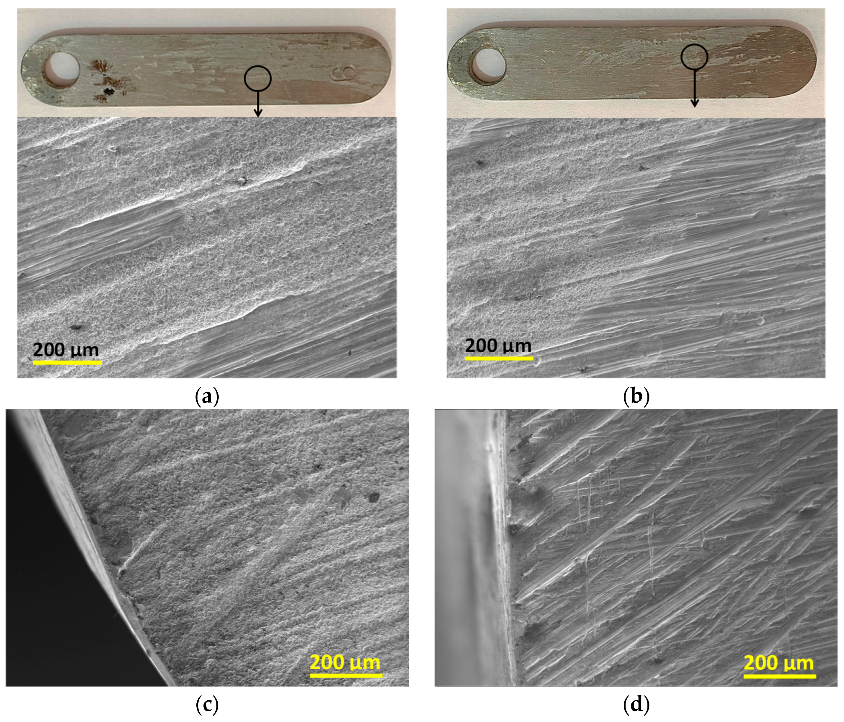
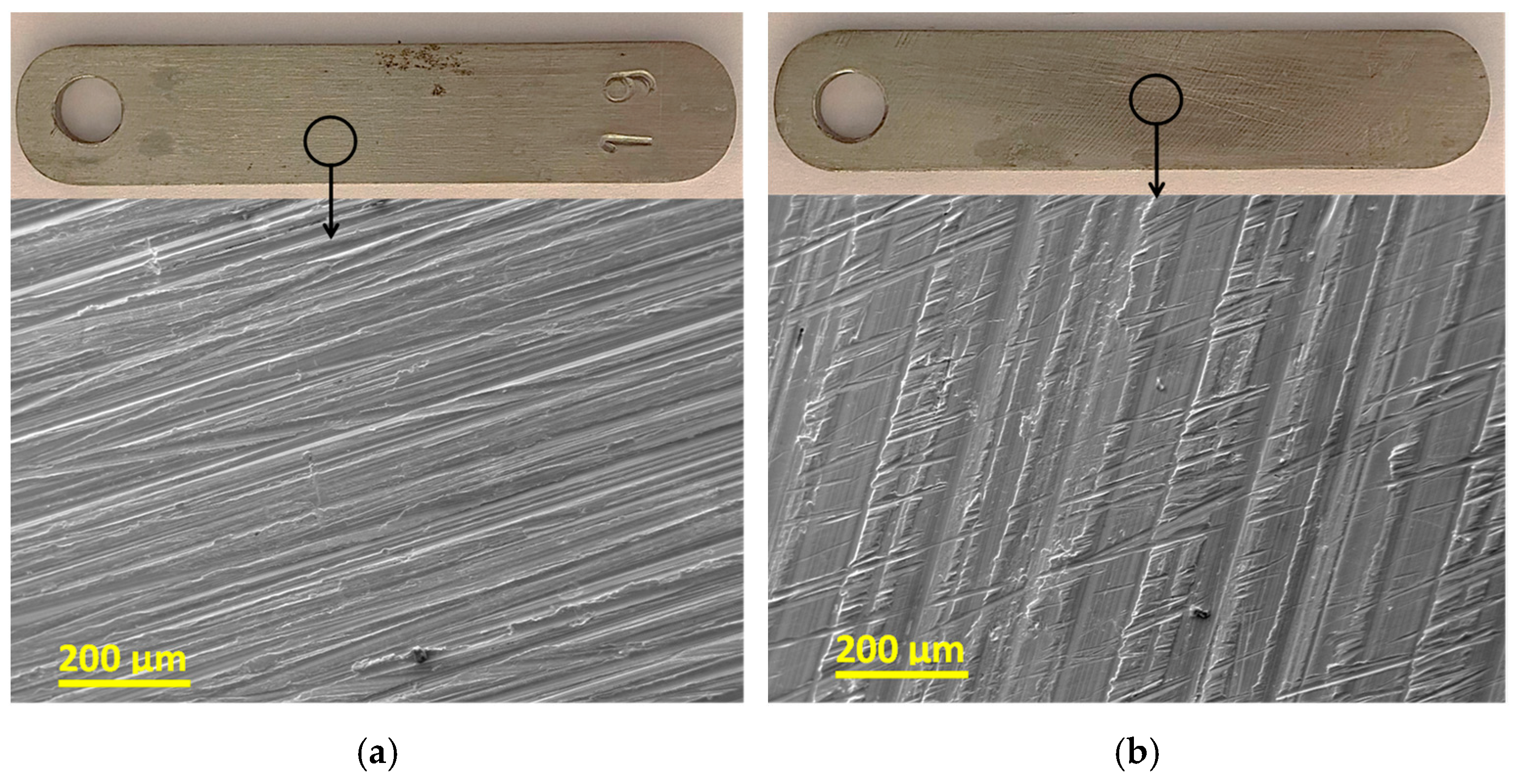
Figure 12 shows the morphological patterns for carbon steel coupons exposed to a flow velocity of 1.4 m s⁻¹ without inhibitor. From this figure, it is evident that the fluid flow patterns influence the rack when the coupons are placed horizontally, with greater degradation observed on the face-up side (Figure 12a) compared to the face-down side (Figure 12b). A similar trend is seen in the ending section of the coupons, where the face-up side (Figure 12c) shows significantly more degradation than the face-down side (Figure 12d).These morphological patterns are consistent with the velocity contours in the y-z plane, as shown in Figure 3a.

Figure 13 shows the corrosion patterns of carbon steel exposed to a flow of OR water containing 20 ppm of inhibitor. As expected, the coupon’s degradation in the presence of the inhibitor is significantly reduced, and the surface polishing is greatly preserved, independently of the face position of the coupons in the experimental rack. As indicated in Table 3, the low corrosion current density can be attributed to the inhibitor’s properties, which limit the diffusion of oxygen molecules from the bulk fluid to the metallic surface.

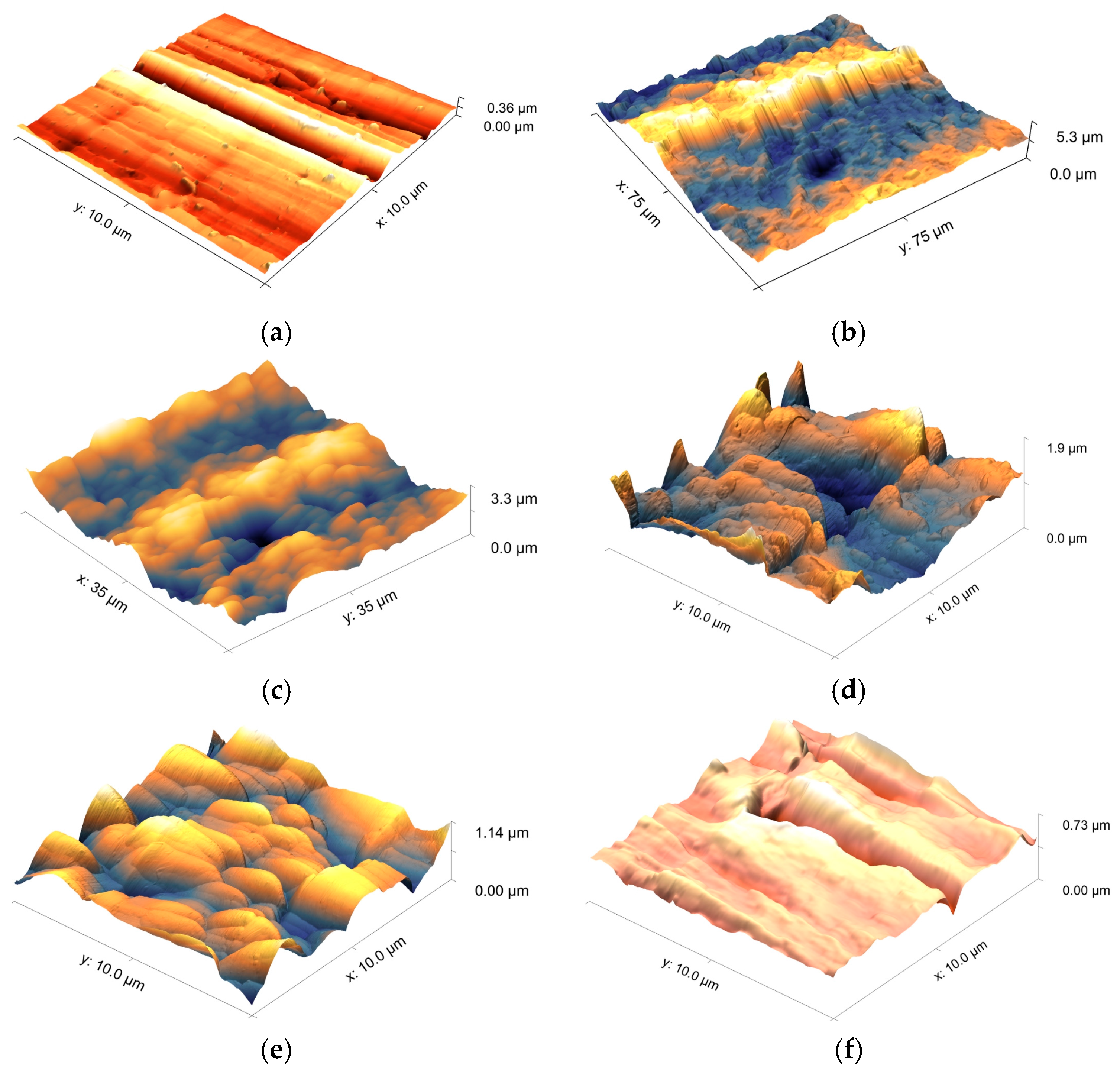
Interestingly, the morphological results did not show localized degradation or pitting on the metallic surface after corrosion. However, in both the inhibited and non-inhibited cases, generalized corrosion was observed on the metallic surface. As shown in Figure 14, AFM images corroborate the corrosion behavior with and without the inhibitor. Before corrosion (Figure 14a), the carbon steel samples show a relative flat surface with a roughness approximately 0.36 μm, attributed to the polishing process.

In the absence of inhibitor (Figure 14b–e), the results clearly show corroded channels with an estimated depth of 5.3 μm (Figure 14b) relative to the uncorroded sites of the surface. Uniform corrosion regions with depths ranging from 1.14 to 1.9 μm (Figure 14a–e) are also observed. In contrast, the results in the presence of inhibitor show no significant differences in topology, with the height gradient reaching values close to 0.71 μm (Figure 14 f–h). The regions also exhibit depths of 0.31 μm, which are like the values observed for the metallic surface before corrosion (Figure 14a).

In this research, the coupon’s rugosity was expected to change with time, both in size and distribution, because of its temporal carbon steel corrosion evolution, while for PVC, rugosity becomes constant at a value of 0.15 μm. From the information gathered from Figure 14 the wall roughness effect can now be estimated. The wall roughness effect in CFD, as in the case of ANSYS Fluent, is characterized by two roughness parameters: the roughness height, which is the average of multiple roughness elements on the surface, and the roughness constant, which is a parameter that measures the uniformity of the roughness. The roughness constant parameter changes from 0.5 to 1; 0.5 indicates a uniform wall roughness, and 1 means strongly non-uniform roughness. As shown in Figure 14a change in roughness height between 0.3 to 4 μm was found. To simplify this complexity, it was decided to fix the roughness height to 2 μm and the roughness constant to 0.5, which corresponds to uniform roughness. Under these conditions a new simulation was almost identical with that of a null roughness height. This confirms the assumption of neglecting the influence of rugosity in CFD simulation.

4. Conclusions

The combined CFD simulation of RO water flow and experimental corrosion studies, including corrosion measurements and morphological characterization of carbon steel planar coupons inside a corrosion rack, led to the following key conclusions:

The k-w CDF turbulent model was successfully applied to characterize the flow dynamics within the corrosion chamber holding a coupon in a testing rack.

The angular position of the coupon along the longitudinal axis of the corrosion rack affected the hydrodynamic distribution and, consequently, the corrosion distribution on the coupon surface at Re > 6000.

The skin friction coefficient was confirmed as an important factor affecting the corrosion rate, primarily by preventing rust accumulation on the coupon surface. The calculated values, between 0 and 0.025, are consistent with those reported in former works.

Experimental corrosion rate values were found to be proportional to the averaged $f$ values obtained for vertical and horizontal coupons. The $f$ values in the coupons and pipe walls are asymmetrically distributed across a vertical x-y plane, with the largest values on both the extrados Tee bend and the face-up coupon surfaces.

The corrosion mechanism considered was a steady-state combination of oxygen mass transfer from the bulk fluid to the coupon surface and a first-order oxygen reduction reaction at the metal surface. These two rate expressions gave rise to an oxygen mass transfer coefficient ($m_c$) and a kinetic rate constant ($k_c$). It was found that lower $m_c$ values occurred in horizontally positioned coupons, while lower $k_c$ values were observed in corrosion runs with the inhibitor. Notably, $m_c$ shows a clear dependency on mass flow magnitude, while $k_c$ appears to be primarily affected by the presence of inhibitors.

In the absence of an inhibitor, the corroded coupon surface exhibited irregular corrosion, characterized by crack-like corroded channels in the fluid direction leaving isolated uncorroded areas. The maximum observed depth channel was 5.3 μm. In the presence of inhibitors, corrosion occurs without corroded channels and at significantly lower rates, with depth close to 0.71 μm.

References

1. ASTM D 2688-05; ASTM International Standard Test Method for Corrosivity of Water in the Absence of Heat Transfer (Weight Loss Method). ASTM International: West Conshohocken, PA, USA, 2005.
2. Benamor, A.; Talkhan, A.G.; Nasser, M.; Hussein, I.; Okonkwo, P.C. Effect of temperature and fluid speed on the corrosion behavior of carbon steel pipeline in Qatari oilfield produced water. J. Electroanal. Chem. 2018, 808, 218–227. [Google Scholar] [CrossRef]
3. El–Gammal, M.; Mazhar, H.; Cotton, J.S.; Shefski, C.; Pietralik, J.; Ching, C.Y. The hydrodynamic effects of single–phase flow on flow accelerated corrosion in a 90-degree elbow. Nucl. Eng. Des. 2010, 240, 1589–1598. [Google Scholar] [CrossRef]
4. Khunphakdee, P.; Chalermsinsuwan, B. Review of flow accelerated corrosion mechanism, numerical analysis, and control measures. Chem. Eng. Res. Des. 2023, 197, 519–535. [Google Scholar] [CrossRef]
5. Xu, T.; Zhang, R.; Si, X. Effects of fluid dynamics parameters on flow-accelerated corrosion at elbow of carbon steel pipeline. Mater. Res. Express 2024, 11, 056520. [Google Scholar] [CrossRef]
6. Elemuren, R.; Evitts, R.; Oguocha, I.; Kennell, G.; Odeshi, A.; Gerspacher, R. Influence of flow velocity on erosion–corrosion performance of 90° carbon steel elbows in potash brine. In Proceedings of the Canadian Society for Mechanical Engineering International Congress, Toronto, ON, Canada, 27–30 May 2018. [Google Scholar]
7. Slaimana, Q.J.M.; Hasan, B.O. Study on corrosion rate of carbon steel pipe under turbulent flow conditions. Can. J. Chem. Eng. 2010, 88, 1114–1120. [Google Scholar] [CrossRef]
8. Si, X.; Zhang, R.; Xu, Q.; Zhou, K. Effects of local velocity components on flow–accelerated corrosion at 90° elbow. Mater. Res. Express 2019, 6, 16557. [Google Scholar] [CrossRef]
9. Moon, S.; Lee, J.; Kim, K.; Han, S.; Lee, G.; Maeng, W. Hydrodynamic parameters affecting flow-accelerated corrosion in elbows. Nucl. Eng. Technol. 2024, 57, 103293. [Google Scholar] [CrossRef]
10. Ansys Fluent; Academic Version 2024 R2; Fluid Simulation Software; Ansys Fluent, Inc.: Canonsburg, PA, USA, 2024.
11. Ko, T.; Choi, H.G.; Bai, R.; Joseph, D.D. Finite element method simulation of turbulent wavy core–annular flows using a k–ω turbulence model method. Int. J. Multiph. Flow 2002, 28, 1205–1222. [Google Scholar] [CrossRef]
12. Wilcox, D.C. Formulation of the k–ω turbulence model revisited. AIAA J. 2008, 46, 2823–2838. [Google Scholar] [CrossRef]
13. Saqr, K.M.; Kassem, H.I.; Aly, H.S.; Wahid, M.A. Computational study of decaying annular vortex flow using the R ε/k–ε turbulence model. Appl. Math. Model. 2012, 36, 4652–4664. [Google Scholar] [CrossRef]
14. Ajmal, T.S.; Arya, S.B.; Udupa, K.R. Effect of hydrodynamics on the flow accelerated corrosion (FAC) and electrochemical impedance behavior of line pipe steel for petroleum industry. Int. J. Press. Vessels Pip. 2019, 174, 42–53. [Google Scholar] [CrossRef]
15. Keshtkar, K.; Nematollahi, M.; Erfaninia, A. CFX study of flow accelerated corrosion via mass transfer coefficient calculation in a double elbow. Int. J. Hydrogen Energy 2016, 41, 7036–7046. [Google Scholar] [CrossRef]
16. Rani, H.P.; Divya, T.; Sahaya, R.R.; Kain, V.; Barua, D.K. CFD study of flow accelerated corrosion in 3D elbows. Ann. Nucl. Energy 2014, 69, 344–351. [Google Scholar] [CrossRef]
17. Martins, F.C.; Pereira, J.M.C.; Pereira, J.C.F. Vorticity transport in laminar steady rotating plumes. Phys. Fluids 2020, 32, 043604. [Google Scholar] [CrossRef]
18. Bao, G.; Qin, W.; Pan, D.; Si, X. Empirical model of flow-accelerated corrosion at elbow of carbon steel pipeline based on dimensional analysis. Ann. Nucl. Energy 2024, 201, 110462. [Google Scholar] [CrossRef]
19. Shoesmith, D.W. Kinetics of Aqueous Corrosion, Corrosion: Fundamentals, Testing, and Protection; ASM International: Russell, OH, USA, 2003; Volume 13A. [Google Scholar]
20. Chilton, T.H.; Colburn, A.P. Mass transfer (absorption) coefficients prediction from data on heat transfer and fluid friction. Ind. Eng. Chem. 1934, 26, 1183–1187. [Google Scholar] [CrossRef]
21. El–Feki, A.A.; Walter, G.W. Corrosion Rate Measurements under Conditions of Mixed Charge Transfer plus Diffusion Control Including the Cathodic Metal Ion Deposition Partial Reaction. Corros. Sci. 2000, 42, 1055–1070. [Google Scholar] [CrossRef]
22. Schmitt, F.G. About Boussinesq’s turbulent viscosity hypothesis: Historical remarks and a direct evaluation of its validity. Comptes Rendus Mécanique 2007, 335, 617–627. [Google Scholar] [CrossRef]
23. Zienkiewicz, O.C.; Taylor, R.; Nithiarasu, P. The Finite Element Method for Fluid Dynamics, 8th ed.; Butterworth–Heinemann: Oxford, UK, 2025. [Google Scholar]
Figure 1. Corrosion testing rack. Experimental closed-loop RO water flow system with two rectangular planar coupons. (A) RO water storage tank, (B) Variable-speed pump controlled by a frequency converter, (C) valve, (D)–(E) bends with plug adapters for steel specimen installation.
Metals 15 00583 g001
Figure 2. (a) Isometric view of the half-symmetric fluid volume geometry inside the compartment containing the rectangular coupon–plastic holder assembly. (b) Path lines across Cartesian x-y symmetry plane at z = 0 used in the flow simulations, where h1 and h8 are along external walls, h4 and h5 are along the coupon surface, h3 and h6 are along the plastic holder and liquid, and h2 and h7 are along the liquid volume.
Metals 15 00583 g002
Figure 3. Normalized velocity magnitude along x-y symmetry plane with coupon at (a) horizontal position and (b) vertical position. Inlet mass flow is 0.28 kg s−1 (run 1).
Metals 15 00583 g003
Figure 4. Normalized velocity magnitude along x lines coupon in a horizontal position (run 1).
Metals 15 00583 g004
Figure 5. Normalized velocity components along x lines shown in Figure 3a: (a) Vx and (b) Vy directions.
Metals 15 00583 g005
Figure 6. z-vorticity at the symmetry plane for horizontally positioned coupon (run 1).
Metals 15 00583 g006
Figure 7. Turbulent kinetic energy along x lines shown in Figure 3.
Metals 15 00583 g007
Figure 8. Specific dissipation rate along x lines shown in Figure 3.
Metals 15 00583 g008
Figure 9. Skin friction coefficient along lines in wall tubing (h1, h8) and coupons (h4, h5) for run 1.
Metals 15 00583 g009
Figure 10. Skin friction coefficient distributions in (a) face-up and (b) face-down sides of horizontally positioned coupon for run 1.
Metals 15 00583 g010
Figure 11. Skin friction coefficient distributions vertically positioned coupon for run 1. Both faces have identical distributions.
Metals 15 00583 g011
Figure 12. Morphological patterns for carbon steel without inhibitor at 1.4 m s−1: (a,c) coupon face-up side, (b,d) coupon face-down side.
Metals 15 00583 g012
Figure 13. Morphological patterns for carbon steel with inhibitor at 1.4 m s−1: (a) coupon face-up side, (b) coupon face-down side.
Metals 15 00583 g013
Figure 14. 3D AFM images for carbon steel in RO water solution at a flow of 1.4 m s−1 (a) before corrosion, (be) in absence of inhibitor, and (fh) in presence of 20 mg L−1 of comercial inhibitor. The coupons were horizontally positioned in the experimental rack.
Metals 15 00583 g014aMetals 15 00583 g014b