Impact of Feature-Selection in a Data-Driven Method for Flow Curve Identification of Sheet Metal

Abstract

This study presents an innovative data-driven methodology to model the hardening behavior of sheet metals across a broad strain range, crucial for understanding sheet metal mechanics. Conventionally, true stress–strain data from such tests are used to analyze plastic flow within the pre-necking regime, often requiring additional experiments to inverse finite element methods, which demand extensive field data for improved accuracy. Although digital image correlation offers precise data, its implementation is costly. To address this, we integrate experimental data from standard tensile tests with a machine-learning approach to estimate the flow curve. Subsequently, we conduct finite element simulations on uniaxial tensile tests, using materials characterized by the Swift constitutive equation to build a comprehensive database. Loading force-gripper displacement curves from these simulations are then transformed into input features for model training. We propose and compare three models—Models A, B, and C—each employing different input feature selections to estimate the flow curve. Experimental validation including uniaxial tensile, plane strain, and simple shear tests on the DP590 and DP780 sheets are then carefully considered. Results demonstrate the effectiveness of our proposed method, with Model C showing the highest efficacy.

1. Introduction

Plastic flow, or plasticity, describes the stress–strain relationship where materials undergo non-reversible shape changes under applied forces. This phenomenon holds paramount importance in various engineering domains, particularly in sheet metal forming processes where materials must be shaped without experiencing failure [1,2,3]. Over recent decades, finite element (FE) analysis has proven effective for designing and validating a part before manufacturing, thus saving time and reducing costs. To ensure the accuracy of FE simulations, it is critical to fist identify an appropriate material model, including its plastic flow behavior.

Conventionally, obtaining data on plastic flow involves conducting standard uniaxial tensile tests to identify parameters of a selected hardening law. However, these conventional methods primarily offer accuracy within the pre-necking range, failing to adequately represent large strain scenarios, such as those encountered in many forming processes like stamping [4], clinching [5], and incremental sheet forming [6]. Consequently, accurate material models for FE simulations require a comprehensive declaration of the stress–strain relationship across a wide range of deformation.

In addition to the conventional uniaxial tensile test, hydraulic bulge tests are commonly used to acquire experimental flow stress data in broad deformation. The stress–strain data obtained from the hydraulic bulge test are derived through the membrane theory [7,8]. Although this method is frequently employed, performing a bulge test is constrained by the inherent limitations resulting from the post-processing assumptions to derive the stress–strain curve from the experiment [9]. In addition, the complex testing apparatus [10] inquired for carrying out the test increases the experimental cost and time.

To address the challenges in identifying post-necking hardening behaviors without conducting an additional test, several inverse methods leveraging FE simulations have been proposed by Mei et al. [11] and Zhao et al. [12]. These methods employ optimization algorithms to minimize the disparity between simulated and realistic material behaviors, often requiring experimental data for validation. Thus, the experimental data are required to provide full-field displacements and strains during the deformation. However, while advanced measurement techniques such as digital image correlation (DIC) can fulfill these requirements, their initial investment costs are substantial [13,14], and local solutions in numerical optimizations may lack outcome uniqueness [15,16,17,18]

Recently, machine learning (ML) techniques that employ statistical learning algorithms to approximate relationships and patterns within a dataset have been applied to calibrate the flow curve of several sheet metals. Bastos et al. [19] proposed a machine learning-based approach to identify material parameters of elastoplastic constitutive models using heterogeneous tests. Jeong et al. [20] proposed several neural network (NN) models to predict uniaxial tensile flow from the load-depth response of indentation tests. In an early work of Pham et al. [21], a method based on machine learning is proposed to estimate the flow curve during the incremental sheet forming (ISF) process up to a plastic strain value of 1.0. Compared to the experimental data, the simulated and measured ISF loading forces exhibit a good agreement with a maximum difference of 5%. In a study by Yamanaka et al. [22], two different deep neural network (DNN) approaches are developed to estimate the biaxial stress–strain curves of aluminum alloy sheets. The high correlation between the biaxial stress–strain curves estimated by the trained DNNs and those calculated by the numerical biaxial tensile tests demonstrate the efficiency of the proposed approaches. These former studies have shown the potential applications of machine learning to identify constitutive models.

Building upon these advancements, this study develops a data-driven method harnessing ML techniques to directly identify the hardening behavior of sheet metals. This method relies solely on the results of a uniaxial tensile test, which is generally insufficient for determining material behavior in the post-necking range using direct experimentation. In addition, a significant advantage of the developed data-driven method is its superior computational efficiency compared to the conventional inverse-modeling approach. The advantage is more superior when considering multiple tasks applied for multiple materials.

The impact of feature selection on the accuracy of the model’s prediction is subsequently highlighted and discussed. To this end, three surrogate models are trained via a database achieved from FE simulations of the standardized uniaxial tensile test to provide the mapping between the material responses and its flow stress curve. Through meticulous model training processes, the capability of these surrogate models to accurately predict the hardening behavior of sheet metal up to large strains is demonstrated. The trained models offer significant time and cost savings in material characterization and identification. Detailed applications of the trained models for DP590 and DP780 sheet metals are presented following further experimental validations. The derived results clarify the potential of the presented data-driven method in practical uses. Moreover, the significance of feature selection of input features in the proposed method is demonstrated by comparing the predictive accuracy of three trained models.

The remainder of this study is detailed as follows. Section 2 gives a brief review of the data-driven methods applied for the identification of material flow stress. Section 3 details the development and training progress of three NN-based surrogate models. Applications of these models for two automotive steel materials, DP590 and DP780 sheets, are presented in Section 4. Section 5 validates the identified flow curves in FE simulations of plane-strain and simple shear tests. Finally, conclusions and discussions are presented in Section 6.

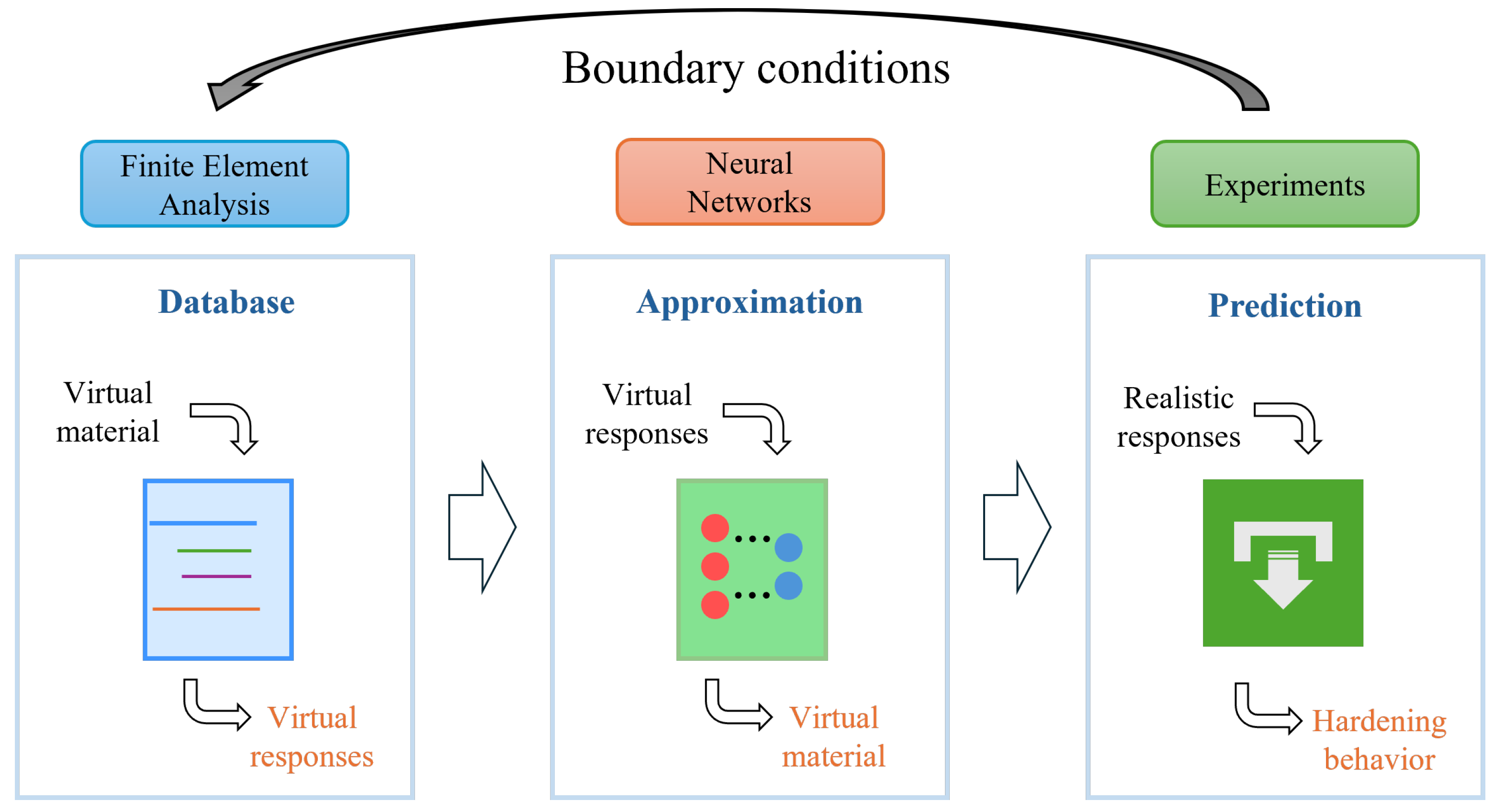
2. Overview of Data-Driven Methods for Plastic Flow Identification

A data-driven approach relies on careful analysis and interpretation of a database to solve problems or make decisions. Within this framework, ML stands out as a prevalent tool to construct surrogate models for modeling the complicated behavior of materials. These ML models strive to regenerate the functional relationships inherent in datasets derived from both high-fidelity simulations and experimental observations through a rigorous training regimen.

A distinction between ML models for learning the plastic flow of sheet metals can be classified into the experimental and numerical data-based models [20,23].

Table 1. Data-driven methods for identification of hardening law of sheet metals.

Group	Ref.	Testing Method	NN Architecture	Input	Output
Group 1	[23]	Compression test	FFNN	$ϵ,\dot{ϵ},T,log\left(ϵ\right),log\left(\dot{ϵ}\right),log\left(T\right)$	$\sigma ,log\left(\sigma \right)$
	[24]	Uniaxial tensile test	FFNN	$\overline{ϵ},\dot{\overline{ϵ}},T,C_{eq}$	${\sigma }^y$
	[25]	Uniaxial tensile test	FFNN	$T,\dot{ϵ},ϵ$	$\sigma$
	[26]	Isothermal CT	FFNN	$T,\dot{ϵ},ϵ$	$\sigma$
	[27]	Uniaxial tensile test	FFNN	$T,\dot{ϵ},ϵ,ln\left(ϵ\right),ln\left(\dot{ϵ}\right),1/T$	$\sigma$
Group 2	[21]	ISF	FFNN	$F,\overline{ϵ}$	Hardening parameters or ${\sigma }^y$
	[22]	Biaxial tensile test	CNN	Images	${\overline{ϵ}}^p,{\sigma }_{max},{ϵ}_{max}^p$
	[28]	TPBT	RNN	F	Hardening parameters
	[29]	Uniaxial tensile test	Decision trees	$F,ϵ$	Hardening parameters
	[30]	Biaxial tensile test	GPR	$F,ϵ$	Hardening parameters

Abbreviations: FFNN, feed-forward neural network; $ϵ$, equivalent strain; $\dot{ϵ}$, strain rate; t, temperature; $\sigma$, equivalent stress; $\overline{ϵ}$, equivalent plastic strain; $\dot{\overline{ϵ}}$, equivalent plastic strain rate; ${\sigma }^y$, yield stress; CT, compression test; $C_{eq}$, carbon equivalent; TPBT, three-point bending test; F, loading force; ISF, incremental sheet forming; RNN, recurrent neural network; CNN, convolutional neural network; ${\overline{ϵ}}^p$, normalized plastic strain; ${\sigma }_{max}$, maximum equivalent stress; ${ϵ}_{max}^p$, maximum plastic strain; GPR, Gaussian process regression.

provides an overview of works in both approaches, with Group 1 and Group 2 denoted as experimental and numerical data-based models, respectively.

Experimental data-based models leverage observational data gathered through experiments as their primary database. Subsequently, neural networks are trained using these data to generate predictive models [24,25,26]. For example, Singh et al. [31] used the experimental stress–strain data to develop ANNs to predict the hot deformation behavior of high-phosphorus steel. In the work of Mohamad et al. [27], an empirical model utilizing an ANN was formulated to forecast the flow curves of ZAM100 magnesium alloy sheets. Although various models based on ML have been proposed within this group [32,33], conducting numerous experiments to generate data to train ML models can be costly and labor-intensive.

In the numerical data-based group of models, NNs are trained through numerical or simulated databases. Numerical simulations are conducted using virtual materials under identical boundary conditions to experimental setups. Subsequently, the NNs are trained to establish the correlation between virtual responses and virtual materials, enabling the estimation of material hardening behavior based on provided experimental data. Figure 1 represents the general methodology of models belonging to this group. Jeong et al. [20] developed surrogate models to predict the stress flow with the load-depth curves obtained from indentation tests. Alternatively, feed-forward neural networks (FFNNs) have been used successfully to estimate a flow curve of sheet metals in incremental sheet forming processes [21]. Recently, Daniel et al. [28] used a recurrent neural network in predicting the material hardening parameters. The results have demonstrated the effectiveness of the methods when evaluated in experimental data. One challenge with these models regards the chosen numerical method possesses sufficient predictive power to accurately represent real-world phenomena of interest. This issue has been addressed to an extent with the development of numerical simulation, especially the finite element method [34,35]. The main benefit of using numerical database models is the computational efficiency brought about by avoiding a large number of experiments.

Taking the advantages of the numerical-database group, this study introduces a data-driven method for predicting the plastic flow stress of sheet metals. Different approaches for selecting input features for training NNs are discussed and implemented. Since inputs are the only information that a trained NN relies on for giving predictions, the accuracy of the inputs is significant for model performance [36,37,38]. For the particular problem of the plastic flow curve identification, insufficient inputs lead to inaccurate predictions, whereas unnecessary inputs misguide the training process and the subsequent predictions. However, the impact of feature selection has rarely been discussed in previous studies.

3. Materials and Methods

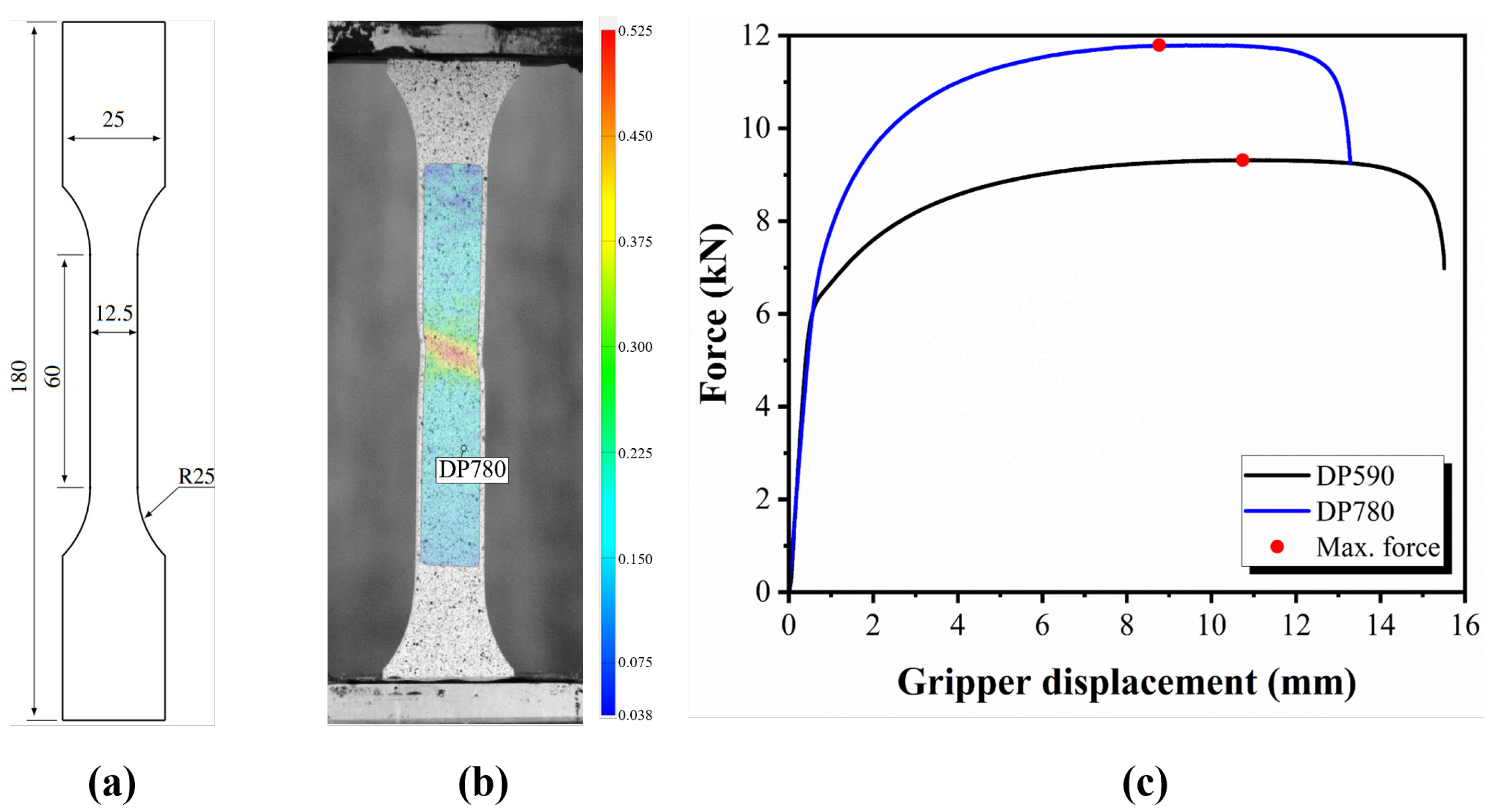
3.1. Uniaxial Tensile Test

The uniaxial tensile test is a prevalent method for assessing the stress–strain relationship of a tested material. Moreover, the stress–strain data derived from the test provide primary information on the material’s hardening behavior. However, the meaningful information is derived in the range of uniform deformation, before the occurrence of plastic instability and strain localization. For thin sheets, the uniform deformation during the uniaxial tensile test often ends at a strain level that is significantly lower than those observed in industrial forming processes, such as stamping, pressing, or bending [6,39]. Recently, the digital image correlation (DIC) method has offered a valuable technique to capture full-field deformation and strain fields across various scales.

In this study, uniaxial tensile tests were performed on DP590 and DP780 sheets, which are widely used in automotive industry. For each tested material, three samples are prepared by a wire cutting machine from a sheet with a thickness of 1.2 mm following the Korean standard KS B0810-13B [40]. Figure 2a illustrates the sample geometries. All specimens were prepared in the rolling direction. The tests are conducted at room temperature with a crosshead speed of 3 mm/min to ensure the quasi-static loading condition. During the tests, the axial loading forces are measured by a loadcell, and the displacement field is captured by a GOM-Correlate 2D DIC system. Figure 2b presents the strain distribution on the surface of a DP780 sample at the onset of fracture. As seen in this figure, the strain level observed at the fractured band is around 0.52, which further exceeds the uniform strain of 0.12 measured at the end of uniform deformation. The comparison demonstrates challenges in deriving the post-necking hardening behavior from the uniaxial tensile test. The mechanical properties of the tested materials are listed in

Table 2. Mechanical properties of tested materials.

Material Properties	DP590	DP780
Young modulus (GPa)	206	206
Initial yield stress (MPa)	409	495
Ultimate tensile strength (MPa)	618	820
Elongation at fracture (%)	25.2	20.4

.

Figure 2 illustrates the gripper displacement versus loading force obtained from these tests. These curves exhibit a consistent pattern: a linear increase in the loading force in the elastic deformation followed by a notable decrease in the rate of increase in force in the plastic deformation until the maximum force, after which the force decreases until the fracture occurs. Additionally, the curves in the linear region exhibit coinciding slopes, indicating a similar Young’s modulus. Consequently, observation of these curves enables a comprehensive characterization of the sheet metals’ hardening behavior.

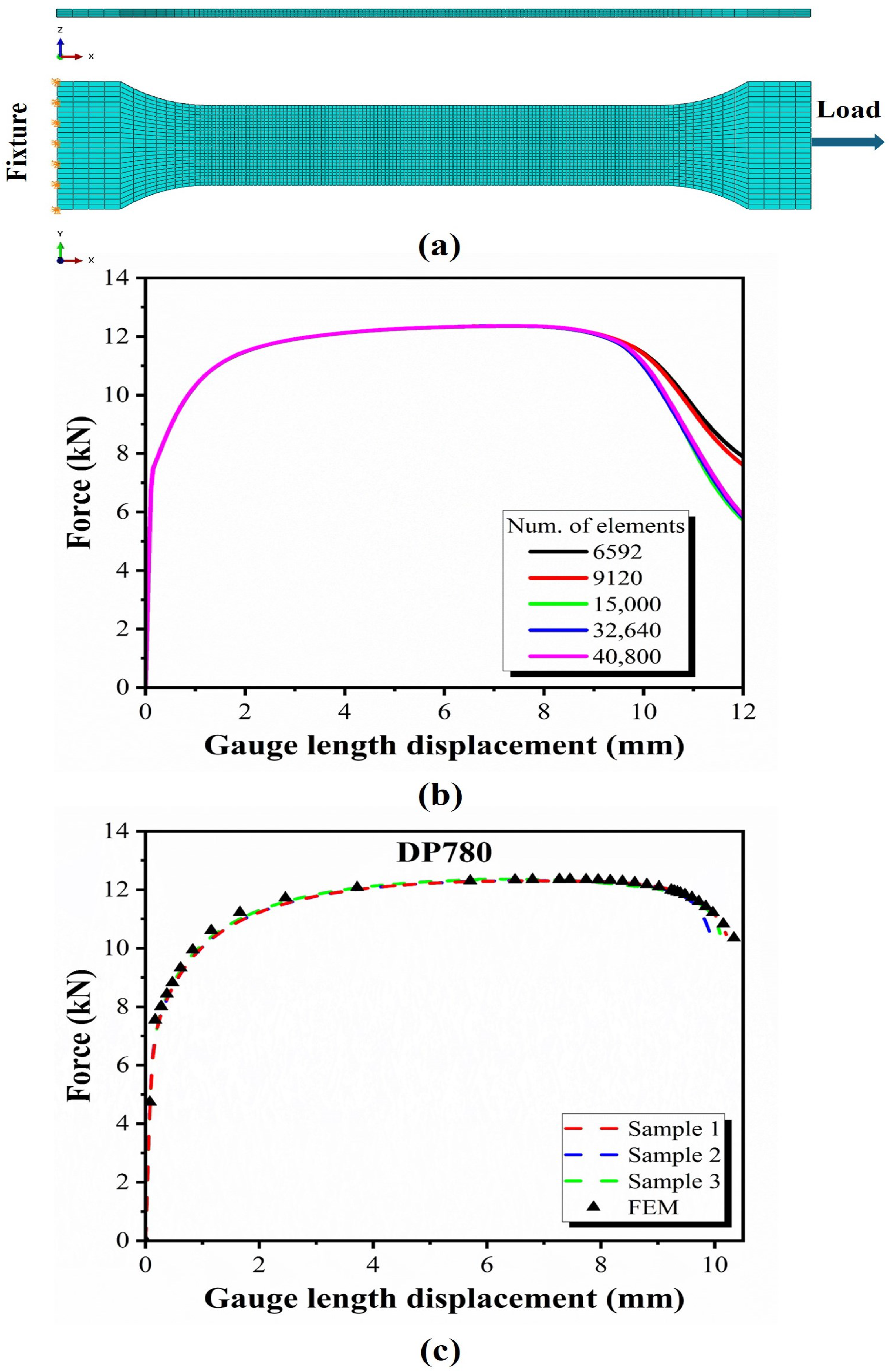
3.2. Finite Element Model

The presented method utilizes a database derived from numerical simulations rather than experimental data. However, this approach inherits the common challenges associated with replacing experiments with simulations. It is crucial to ensure that the chosen method possesses sufficiently to reproduce the real-world problem accurately. Building on its exceptional ability to accurately predict material responses during uniaxial tensile tests, as demonstrated in previous studies [20,40,41,42], the FE method proves to be a robust and reliable approach for establishing a database for the proposed method.

In this study, numerical data obtained from simulations of uniaxial tensile test serve as the database, necessitating careful development of an FE model for the tensile test. Following the findings in [20], the material models are isotropic and the Von Mises yield criterion is adopted. Young’s modulus and Poisson’s ratio are assumed to be 206 GPa, and 0.3, respectively, which are reported in the previous studies [43,44,45,46,47,48] for various steel types. To describe the flow curve of material, the Swift model [49] is considered which effectively captures the hardening behavior, as expressed below:

$$\mathrm{Swift}:\overline{\sigma }=\kappa {({\epsilon }_0+{\overline{\epsilon }}_p)}^n$$

(1)

where $\kappa$ is strength coefficient, ${\epsilon }_0$ is strain hardening exponent, and n is strain parameter.

The specimen’s geometry used in the FE model is followed by that of the experimental specimens aforementioned in Section 3.1. First-order solid elements with reduced integration (C3D8R) in Abaqus/Standard are chosen to generate the mesh of the sample. The effects of strain rate and temperature are totally ignored in the simulations. Moreover, the mesh of the reduced section is intentionally finer, and the mesh is made progressively coarser further toward the grippers. The model is configured to apply tension load to the specimen from the left, while the left section is fixed to emulate the relative uniaxial motion between the two grippers of a tensile testing machine. The FE model with meshing and boundary conditions is presented in Figure 3a. A mesh convergence study is carried out and confirms that the FE model achieves convergence at 15,000 elements, as shown in Figure 3b.

Ensuring the accuracy of the FE model is paramount for the proposed method. Therefore, the derived numerical results are compared with the experimental data, as depicted in Figure 3c. The identified hardening law of the Swift model is imposed on the developed FE model to simulate the uniaxial tensile test. After simulation, the predicted loading forces are collected and compared to the experimental data. A good agreement between the simulated and measured forces is achieved. The comparison verifies the capability of the FE model to capture material responses over a wide strain range.

3.3. Surrogate Model

This section details the procedure for developing surrogate models, encompassing both data collection and model development. The surrogate models are developed via a training neural network that completely leverages loading force-gripper displacement data and produces the outputs regarding the flow curve.

3.3.1. Data Acquisition

A series of simulations are performed to acquire a database for NN training. Following the previous study [20], the simulations incorporate variations in the hardening behavior of the material through the manipulation of parameters, i.e., $\kappa$, ${\epsilon }_0$, and n of the Swift constitutive model. According to this study, the entire parameter space is defined as $D=[800,2150]\times [0.001,0.073]\times [0.05,0.59]$. The parameter design space is considered to sufficiently capture the hardening behaviors of a wide range of steels, which are mainly used in the automotive industry. Therefore, a total of 1000 simulations are performed with different hardening behaviors by randomly combining the constitutive parameters using the Latin Hypercube Sampling (LHS) method.

During the simulations, loading forces and gripper displacements are recorded, and a typical result is plotted in Figure 4 as an illustration. In addition, three points, namely $P_1$, $P_2$, and $P_3$, are determined and plotted in this figure. $P_1$ represents the point at which the relationship between loading force and gripper displacement starts being non-linear; $P_2$ corresponds to the maximum loading force, and $P_3$ is the point at which the force is at 95% of the maximum force. Physically, one may associate $P_1$ to the initial yield stress of the tested material, while $P_2$ relates its tensile strength. Moreover, the point $P_3$ regards the hardening behavior at large strains [40]. Therefore, these points facilitate important features for training neural networks.

In this study, three surrogate models are developed to predict the plastic flow stresses of sheet metals represented by discrete data points. Instead of estimating the parameters of the hardening model, the predicted flow stresses are inferred from the equivalent plastic strains fed to the input features. Following the procedure presented in [21], the evaluated values of equivalent plastic strain are in the interval [0, 1] with an increment of 0.01 and 50 other random values. The detailed procedure for generating the dataset and developing a neural network for each model is elucidated in the following subsections.

3.3.2. Feature Selection

The development of three surrogate models emphasizes the advantages of feature selection for the model’s inputs, which aim to reproduce precisely the material responses. In this study, the simulated force–displacement curves outline the virtual material responses. Figure 4 presents a typical curve obtained from a random case. The feature selection needs to strategically enhance predictive performance and improve robustness of the surrogate models by selecting the most informative features while discarding redundant features to rebuild the material responses.

Model A

Naturally, a curve can be represented by a series of consecutive points, which inspires a strategy to use force points directly as input features. Although this approach has been successfully employed in previous studies [19,20,28], this work introduces a simple modification by selecting three key points, $P_1$, $P_2$, and $P_3$ as input features to enhance their influence on model predictions. As a result, twenty-four features are designated as model inputs, including three forces specified at $P_1$, $P_2$, and $P_3$ along with nineteen force values corresponding to consecutive displacements between $P_1$ and $P_3$. In addition, the input features of Model A contain two extra components: the displacement value at $P_2$ and the examined equivalent plastic strain (${\overline{\epsilon }}^{*}$). The displacement at $P_2$, together with its force, provides essential information about the flow curve at diffuse necking. Accurately predicting this point is crucial not only for calibrating the post-necking hardening behavior of the tested material but also for evaluating its formability [50,51].

Model B

As seen in Figure 4, the curve between $P_1$ and $P_3$ could be perhaps described by certain functions. Various functions, i.e., quadratic, cubic and quartic functions, are tried to fit the data within the ranges from $P_1$ to $P_2$ and from $P_2$ to $P_3$, respectively. Consequently, the coefficient of determination ($R^2$) is used to inspect the fitting goodness. The formula of $R^2$ is expressed as follows:

$$R^2=1-{\displaystyle \frac{{\sum }_{i=1}^N{(y_i-{\widehat{y}}_i)}^2}{{\sum }_{i=1}^N{(y_i-\overline{y})}^2}}$$

(2)

where $y_i$ and ${\widehat{y}}_i$ are observed and predicted values, respectively; $\overline{y}$ denotes the mean of the observed values; and N is the number of observations.

The comparison demonstrates a strong fit of a quadratic function for the data of both ranges. Figure 5 presents the distribution of $R^2$ calculated based on the fitting of the quadratic function for the dataset obtained from 1000 simulations. For the segment between $P_1$ and $P_2$, the mean and standard deviation of $R^2$ are 0.9894 and 0.0075, respectively, while those of $R^2$ for the curve between $P_2$ and $P_3$ are 0.9929 and 0.0023, respectively. Moreover, it is seen that $R^2>0.95$ for all simulated data. Therefore, the quadratic function is adopted to approximate the simulated data and extract input features. For a clear and simple notation, the quadratic functions fitted to $P_1$–$P_2$ range and $P_2$–$P_3$ range are symbolized by $f_1$ and $f_2$. The formula of these quadratic functions is expressed as follows:

$$f_1=a_1{x}^2+b_{1}x+c_1$$

(3a)

$$f_2=a_2{x}^2+b_{2}x+c_2$$

(3b)

where $a_{1,2}$, $b_{1,2}$ and $c_{1,2}$ are coefficients.

Afterwards, inputs of Model B contain the information of three key points $P_1$, $P_2$, and $P_3$; coefficients of two quadratic functions $f_1$ and $f_2$; and the examined ${\overline{\epsilon }}^{*}$. In total, Model B consists of 11 features.

Model C

Model C is developed with a further reduction in the number of input features. Thought that the force value at $P_3$ is depended on that of $P_3$. In addition, the displacement at $P_1$ is unnecessary because this point is associated with the initial yield stress of the identified flow curve. Therefore, these two features are removed in Model C. Normalization of the displacement values of $P_2$ and $P_3$ may avoid the effect of dimensionality and enhance the robustness of the training process.

Moreover, coefficients $a_1$ and $b_1$ can be used to reproduce the first derivative of $f_1$, which is associated with the hardening rate of the flow curve, denoted by ${\displaystyle \frac{d\overline{\sigma }}{d\overline{\epsilon }}}$. Under the diffuse necking condition, the following condition is hold:

$$\mathrm{Diffuse}\mathrm{neck}:\overline{\sigma }={\displaystyle \frac{d\overline{\sigma }}{d\overline{\epsilon }}}$$

(4)

The information regarding the diffuse neck has been completely provided by the point $P_2$. Introducing the $b_1$ as a feature may add unnecessary constraints in calculating the weights of the surrogate model. Therefore, inputs of Model C contain 7 features, as summary in

Table 3. The descriptions for determining the input features of surrogate models.

Model	Input Feature	Description
Model A	$X_1$	Force at $P_1$
	$X_2$	Force at $P_2$
	$X_3$	Force at $P_3$
	$X_4\sim X_{22}$	Forces at 19 consecutive displacements between $P_1$ and $P_3$
	$X_{23}$	Gripper displacement at $P_2$
	$X_{24}$	Examined ${\overline{\epsilon }}^{*}$
Model B	$X_1$	Force at $P_1$
	$X_2$	Gripper displacement at $P_1$
	$X_3$	Force at $P_2$
	$X_4$	Gripper displacement at $P_2$
	$X_5$	Force at $P_3$
	$X_6$	Gripper displacement at $P_3$
	$X_7$ and $X_8$	Coefficients a and b of $f_1$
	$X_9$ and $X_{10}$	Coefficients a and b of $f_2$
	$X_{11}$	Examined ${\overline{\epsilon }}^{*}$
Model C	$X_1$	Force at $P_1$
	$X_2$	Force at $P_2$
	$X_3$	Ratio between the gripper displacement at $P_2$ and the sample’s initial length
	$X_4$	Ratio between the gripper displacement at $P_3$ and the gripper displacement at $P_2$
	$X_5$	Second derivative of $f_1$
	$X_6$	Second derivative of $f_2$
	$X_7$	Examined $\overline{\epsilon }$*

.

3.3.3. Neural Network Architecture

The surrogate models are constructed using multi-layer perceptrons (MLPs), a type of artificial neural network. An MLP consists of an input layer, hidden layers, and an output layer, where each layer is fully connected to the sequential layer. An activation function is applied to units in the hidden and output layers to introduce non-linearity. This algorithm allows learning by updating weights and biases through a back-propagation algorithm. Due to its architecture, MLP effectively approximates complex non-linear problems. Previous studies have highlighted the importance of adjusting hyperparameters, such as the number of hidden layers and the number of units per layer, to improve the generalization of neural network models [20,52]. In this context, these parameters are optimized to appropriate values, and hyperparameter turning process for surrogate models is detailed in Appendix A.

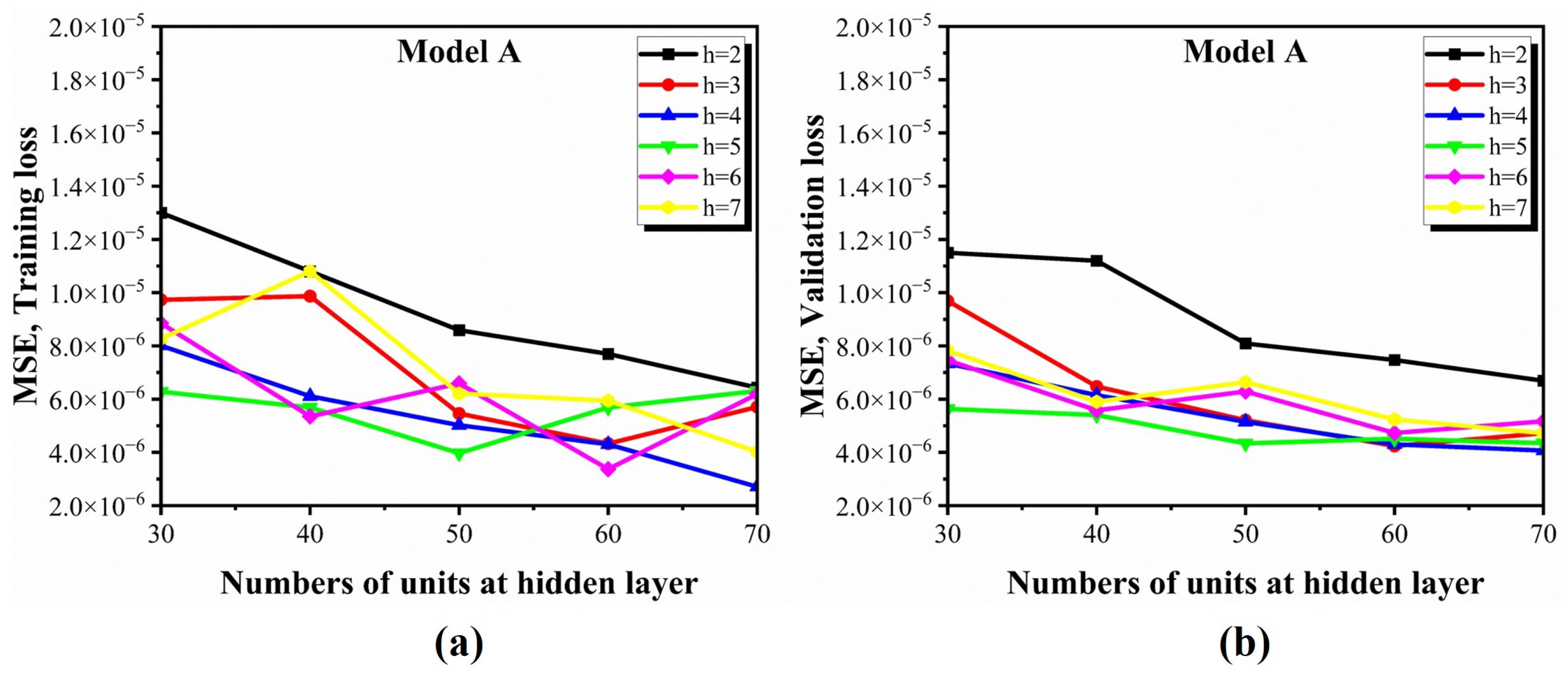
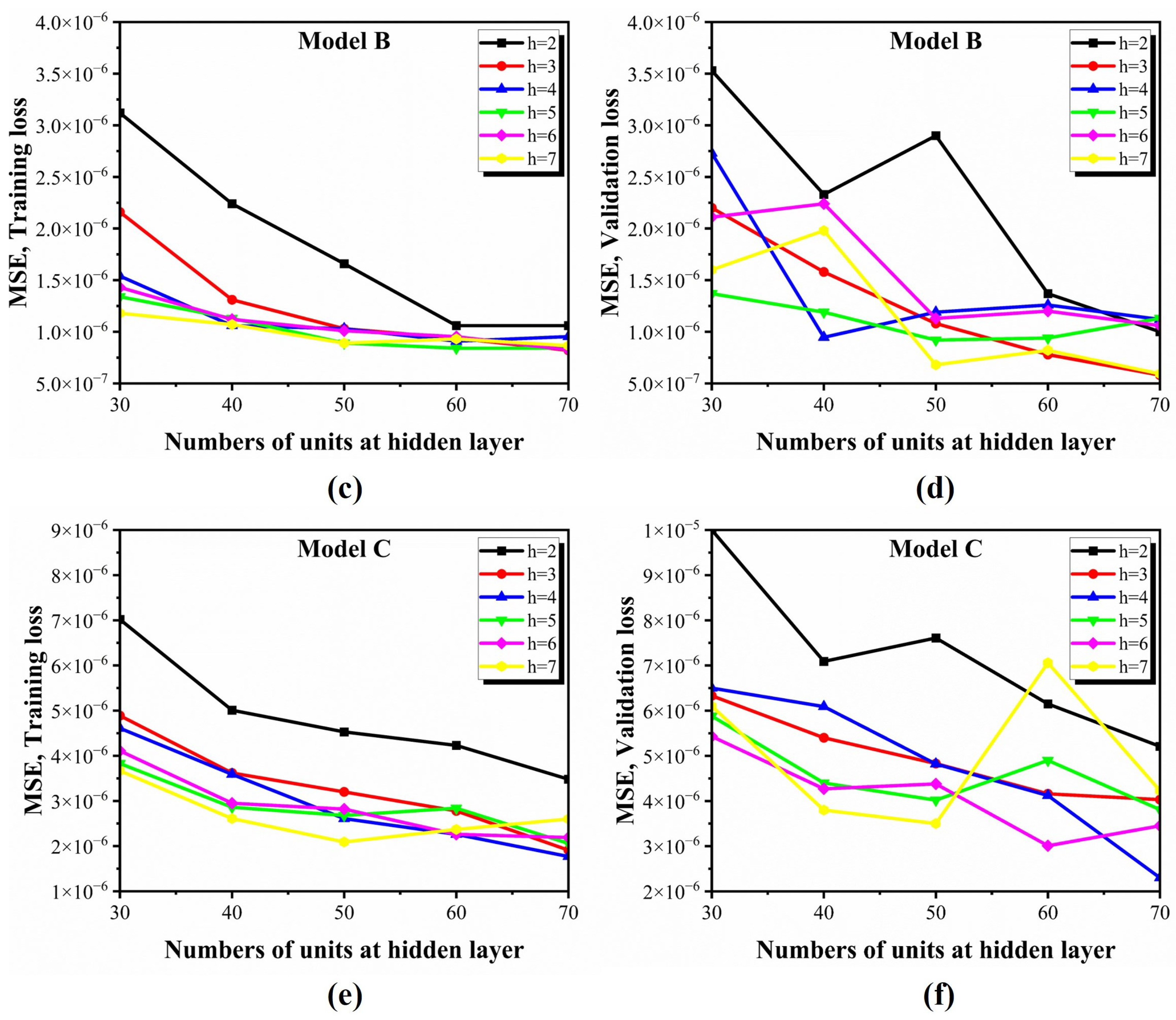
3.4. Training and Validation

The entire dataset of each model has been randomly split into train/validation/test sets with ratios of 80:10:10%, respectively. The NNs are trained in a supervised way by minimizing the difference between the predicted values ${\widehat{\mathbf{y}}}_i$ and true values ${\mathbf{y}}_i$ through the mean square error (MSE) criterion. The formulation of MSE is expressed as:

$$MSE={\displaystyle \frac{1}{M}}\sum _{i=1}^M{({\widehat{\mathbf{y}}}_i-{\mathbf{y}}_i)}^2$$

(5)

where M denotes the number of data for training and validation.

Before training, the ground truth features are normalized to range (0, 1). Weights and bias of each model are optimized using the Adam optimizer [53], with a learning rate of $3\times {10}^{-4}$. The Rectified Linear Units (ReLUs) [54] are adopted as the non-linear activation function throughout the network.

Three models are implemented using TensorFlow (2.16.1) [55] and the neural networks are trained using mini-batch gradient descent with a batch size of 128, leveraging its advantages in enhancing generalization performance and improving computational efficiency [56]. The training process is terminated by an early stopping criterion when the MSE on the validation dataset remains unchanged after 100 epochs. In addition, a model checkpoint function is employed to store the learning parameters at the point of achieving the lowest validation loss, ensuring that the optimal model configuration is preserved.

The loss values for the training and validation sets, recorded during the training process, are shown in Figure 6a,c,e. Model A exhibits high fluctuations in both training loss and validation loss, indicating potential overfitting and instability. In contrast, Model B demonstrates more stable variations, while Model C shows the smoothest and most stable training behavior. The input features in the models represent material responses, and increasing the number of features increases the complexity of the model. This higher complexity increases the model’s sensitivity to noise in the measured data, leading to greater variance and a higher likelihood of overfitting. Furthermore, excessive sensitivity to noise can make optimization more challenging, potentially contributing to training instability. Despite the differences in training behavior, all three models achieve good generalization because they ultimately capture the essential material response patterns, allowing them to perform well on the test set (Figure 6b,d,f). For easy reference,

Table 4. Training results of the surrogate models.

	Model A	Model B	Model C
Input layer	$\mathbf{X}={[X_1,\dots ,X_{24}]}^T$	$\mathbf{X}={[X_1,\dots ,X_{11}]}^T$	$\mathbf{X}={[X_1,\dots ,X_7]}^T$
Target output	$\widehat{\mathbf{Y}}=\left[{\sigma }^y\left({\overline{\epsilon }}^{*}\right)\right]$
Architecture	4 hidden layers, 70 nodes per each	3 hidden layers, 70 nodes per each	4 hidden layers, 70 nodes per each
Epoch	1172	941	1227
Training loss	$4.38\times {10}^{-6}$	$7.64\times {10}^{-7}$	$1.95\times {10}^{-6}$
Validation loss	$4.92\times {10}^{-6}$	$8.69\times {10}^{-7}$	$3.23\times {10}^{-6}$
Test dataset valuation	$R^2>0.9999$	$R^2>0.9999$	$R^2>0.9999$
Training time	17 min	23 min	30 min
CPU	CPU i7-12700F, 2.10 GHz, 48 GB RAM, Window 10 Pro

The average values obtained from 100 training individuals.

summarizes the network configuration and the performance of the three models.

4. Application

In this section, the performance of three developed models is investigated on DP590 and DP780 sheets. Initially, loading force-gripper displacement values reported in “Section 3.1” of the tested materials are transformed into input features for these models. Subsequently, these features are fed into the input layer of the models to estimate the outputs. A detailed comparison between the predicted flow stresses with the experimental data is also discussed.

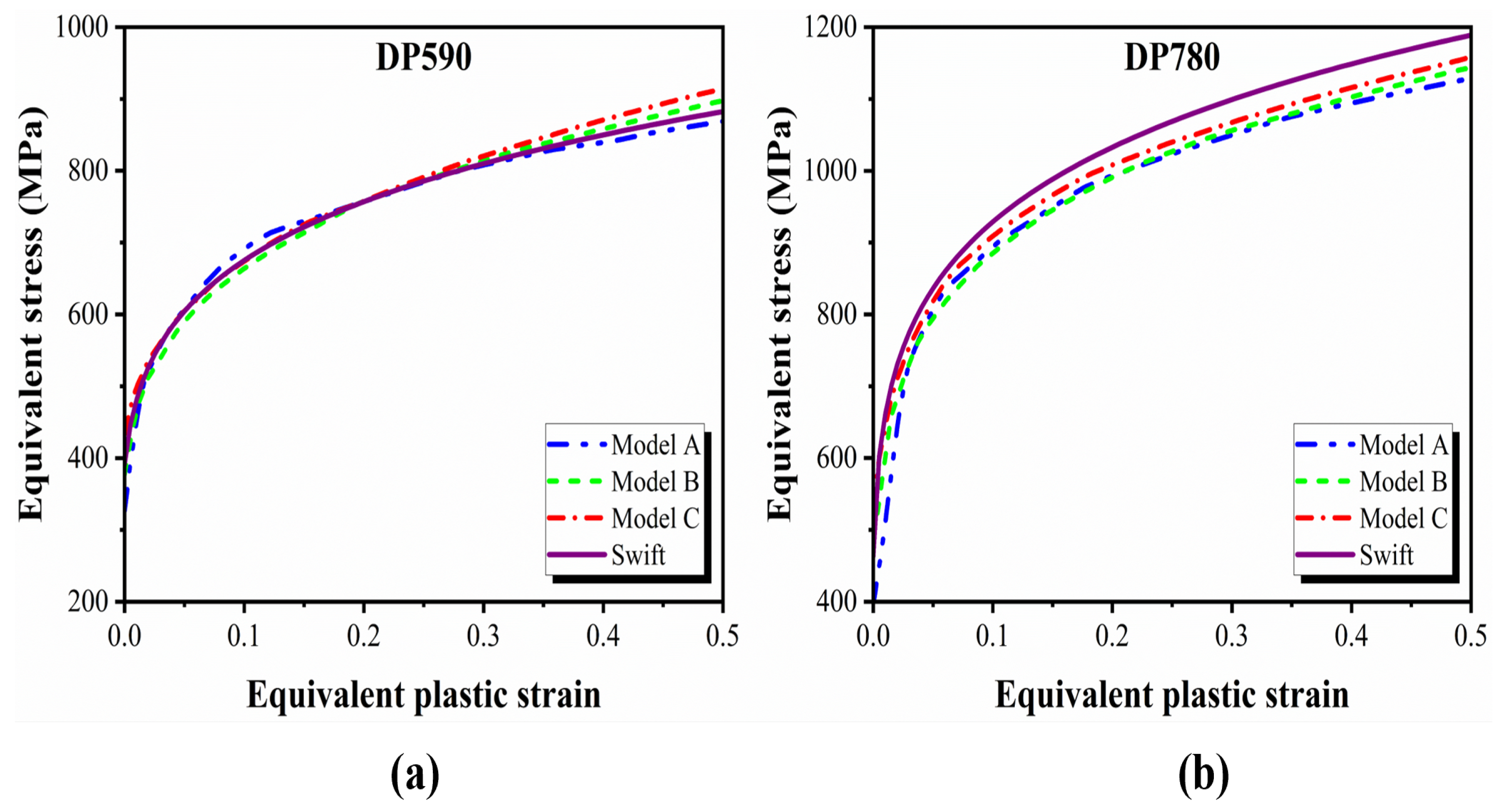
4.1. Flow Stress in the Pre-Necking Range

To assess the performance of these models in pre-necking strain ranges, flow stress curves measured by uniaxial tensile tests are compared with those predicted by the three ML models. Figure 7a,b illustrates how these ML models infer the hardening behavior of steel materials.

According to Figure 7a, all model predictions agree well with the experimental data for DP590 sheets. Compared to the uniaxial tensile test data for this material, the coefficients of determinations, $R^2$, based on Models A, B, C are 0.964, 0.973, and 0.988, respectively. In contrast, Model A’s prediction for the flow stresses of the DP780 sheet deviated significantly from the experimental data, as shown in Figure 7b. Meanwhile, Model B and Model C provide more accurate predictions for this material, with $R^2=0.783$ and $R^2=0.944$, respectively. Generally, the performance of Model B and C is superior to that of Model A. The observation can be attributed to the reduction in redundant features in the input layers of the former. Additionally, Model A’s reliance on direct material response as input data makes it more susceptible to noise in experimental measurements. Therefore, the approach used to reduce the number of input features of Models B and C may effectively eliminate redundant information feeding into neural networks in similar problems.

Besides the evolution of the effective stress with respect to the effective plastic strain, its derivative is also important for understanding material behaviors when they are subjected to external loads. Therefore, the numerical derivative of the predicted flow stress based on three models is calculated and presented in Figure 7c,d. In this manner, the stress derivative is approximated by the forward difference as follows:

$$\begin{array}{c}\hfill {\displaystyle \frac{d\overline{\sigma }}{d{\overline{\epsilon }}_i}}\approx {\displaystyle \frac{\overline{\sigma }\left({\overline{\epsilon }}_{i+1}\right)-\overline{\sigma }\left({\overline{\epsilon }}_i\right)}{{\overline{\epsilon }}_{i+1}-{\overline{\epsilon }}_i}}\end{array}$$

(6)

where ${\overline{\epsilon }}_i$ and ${\overline{\epsilon }}_{i+1}$ are two consecutive equivalent plastic strains derived from the flow curve. Similar to their prediction on the flow stresses, three models provide fairly good predictions for the stress derivative of the DP590 sheet. However, the predictions of Model A and Model B for the DP780 sheet exhibit an abrupt increase in the early stage of deformation, i.e., near $\overline{\epsilon }=0.02$, followed by a decrease. The increase in the derivative curves infers an unsmooth in the flow stress curves, which may yield difficulties in the convergence of the corresponding numerical simulations. Future studies on this topic may consider involving the stress derivative in the loss function to improve the performance of the trained network.

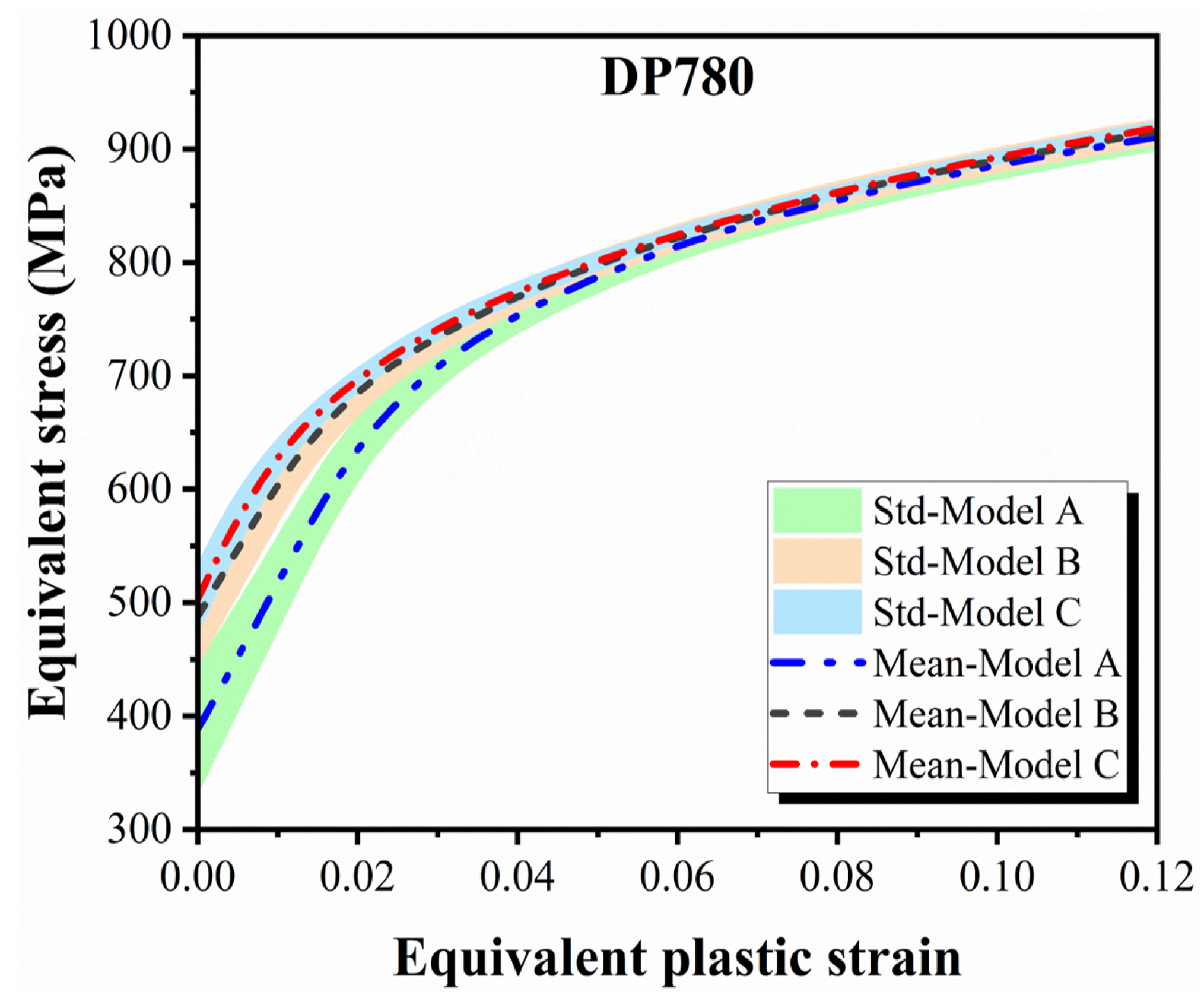
4.2. Flow Stress in the Post-Necking Range

It is a high demand on accurately predicting the post-necking hardening behavior of sheet metals subjected to forming processes like stamping, bending, hydroforming, and deep-drawing [57]. To investigate the capacity of three surrogate models in forecasting the post-necking behavior, their predicted flow curves are shown in Figure 8 up to a strain of 0.5. In general, the three models produce similar results for flow stresses in the post-necking range, closely following the power laws. Notably, the flow curves predicted by these models are represented by discrete points, confirming the reliability of the developed data-driven method.

In more detail, Model C consistently shows the highest stress values for both DP590 and DP780 sheets in the large strain ranges. Model B follows closely behind, while Model A exhibits the lowest stress values among the three models. As strain increases, the differences between the model predictions become more pronounced. The divergence confirms the influences of feature selection on the model prediction.

Comparisons in Figure 7 indicate that Model C consistently outperforms Models A and B in predicting the flow stresses of the tested materials, despite having the fewest input features. As a conclusion, the quality of input features has a greater impact on model performance than their quantity. Ideally, all input features should be independent to provide novel information to the network. One potential approach is to use feature selection algorithms, such as Principal Component Analysis or Recursive Feature Elimination, to optimize model inputs. However, these algorithms are computationally expensive and struggle to handle nonlinear relationships [58]. Alternatively, autoencoder algorithms can be used to reduce the number of dependent features [20]. However, this approach treats the neural network as a black box, posing challenges in the explainability of the developed model. In this study, we introduce a feature selection approach based on the physical significance of the features, as presented in Model C. For this particular problem, the approach not only reduces the number of input features but also increases the performance of the developed surrogate model.

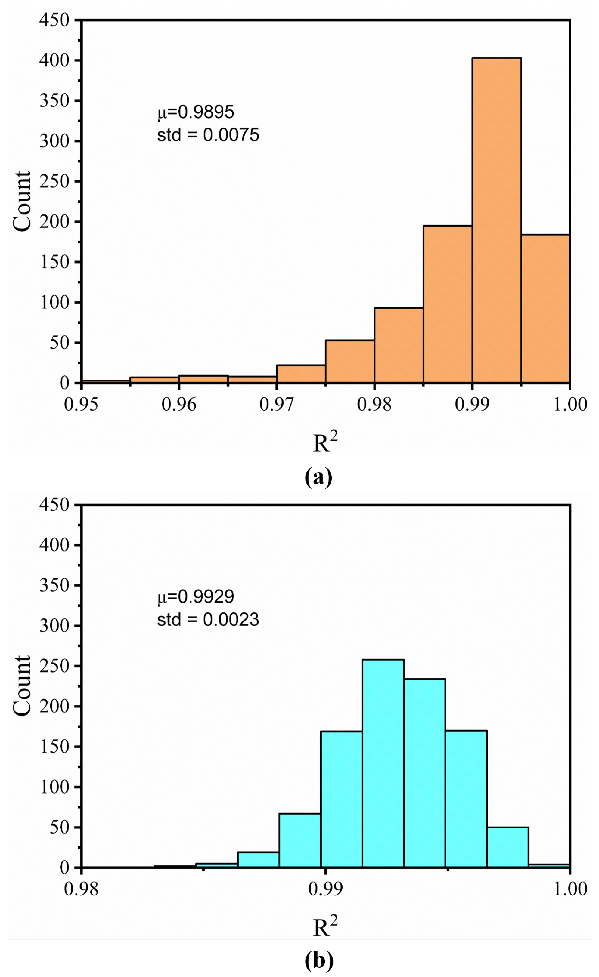
4.3. Repeatability of the Training Process

To appraise the robustness of three models, each model has been trained repeatedly 100 times. The $R^2$ coefficients were utilized to compare their performance in pre-necking strain ranges, as reported in

Table 5. Statistical values over 100 training individuals for robustness evaluation of three developed models based on their prediction for the unseen test set.

Model	DP590	DP780
	${\mathit{R}}^{\mathbf{2}}$	${\mathit{R}}^{\mathbf{2}}$
A	0.970 ± 0.028	0.448 ± 0.253
B	0.967 ± 0.030	0.775 ± 0.112
C	0.979 ± 0.014	0.838 ± 0.056

. The comparison reveals distinct differences in accuracy and robustness for DP590 and DP780 sheets. As seen in the table, Model C demonstrates superior accuracy for both two materials along with the lowest standard deviation. For DP590 sheets, the robustness of three models are similar, indicated by similar $R^2$ values reported in Table 5. Notice that the variations of the three models are small, demonstrating their good predictions for the flow stress in the pre-necking ranges. However, the robustness of these models in predicting the flow stress of DP780 are diverse significantly. Model A exhibits low consistency with a low $R^2$ of 0.448 and a high standard deviation of 0.253. Models B and C show $R^2=0.775\pm 0.112$ and $R^2=0.838\pm 0.056$, respectively. The comparisons highlight the critical role of feature selection in the developed data-driven method, particularly for materials exhibiting complex hardening behavior, such as DP780 sheets. Model A assigned equal importance to all force points between $P_1$ and $P_3$, whereas Models B and C significantly emphasized the contribution of key points, namely $P_1$, $P_2$, and $P_3$. Consequently, Model A exhibits greater variation in the predicted initial yield stress compared to the other models, as shown in Figure 9. Additionally, the mean predicted initial yield stress of Model A is significantly lower than the experimental data, whereas the prediction of Model C closely aligns with the experimental mean. That makes Model B (and Model C) a more reliable choice over Model A.

5. Validation

The objective of this section is to evaluate the predictions of Model A, Model B, and Model C over large strain ranges. For this purpose, predicted flow curves of DP590 and DP780 sheets reported in Section 4 are applied to simulate the plane-strain and simple shear tests using the Abaqus/Explicit package. Then, the predicted loading forces are compared to experimental data to validate the accuracy. In this work, the geometries of specimens used in [40] are adopted, as shown in Figure 10a. The tests are conducted at room temperature and under a quasi-static condition. To ensure the conditions, the samples were pulled with a speed of 1 mm/min until fracture. During tests, loading forces were recorded by the load cell, whereas the displacements of a virtual extensometer were analyzed via the DIC technique. Details on constructing the virtual extensometer were discussed in the previous study [40].

In the numerical simulations, only one-half of the simple shear specimen is considered, while the full thickness of the plane-strain specimen is depicted. Consequently, a Z-symmetric boundary condition is implemented to simulate the simple shear specimen in the thickness direction. The meshing process is presented in detail in [40] and the numerical models were developed using ABAQUS software. The mesh on the critical areas of the samples used in the simulations is shown in Figure 10a.

The load–displacement curves for the plane-strain and simple shear tests of DP590 and DP780 sheets are shown in Figure 10b–e. According to Figure 10b, the performances of the three models examined in the simple shear test simulation for DP590 sheets are similar. However, their performances on simulations of the plane-strain test exhibit significant differences, as seen in Figure 10d. In detail, Model C shows the best agreement with the experimental data in both tests. Model B also performs well but deviates slightly from the experimental data, while Model A significantly underestimates the loading forces.

In the simple shear test simulations for DP780 sheets (see Figure 10c), both Model B and Model C yield similar predictions of the loading force, which closely match the experimental data, whereas Model A exhibits a significant deviation. In the plane-strain test, Model C achieves the best agreement with the experimental data, followed by Model B. Similarly, Model A demonstrates poor predictive performance. In general, Model C presents the best performance and stability, followed by Model B, with Model A being the least accurate.

6. Conclusions and Discussion

6.1. Discussion

This study examined the impact of feature selection in a data-driven approach for flow stress identification in sheet metal. The developed models successfully demonstrated their ability to predict the hardening behavior of two steel sheets (DP590 and DP780) up to an effective plastic strain of 0.5 using force–displacement data from uniaxial tensile tests. Due to its computational efficiency, the developed surrogate model can be integrated into a cloud-based platform to accelerate the material identification process [59,60]. This integration may help simplify user interactions with modeling and simulation of metal forming processes using existing computer-aided engineering tools. Additionally, a high-fidelity database that properly combines numerically simulated and experimentally measured data will provide enriched information for training surrogate models and improving prediction accuracy. It is believed that the data-driven method will soon deliver results as accurate as those obtained through conventional material identification approaches. However, the former surpasses the latter in computational efficiency and consistency. Consequently, this method exposes a high potential of being implemented in high-throughput testing platforms for industrial-scale material characterization.

All of the neural networks in this study are built upon multilayer perceptrons. In contrast to MLPs, recurrent neural networks (RNNs), known for their effectiveness in modeling sequential tasks, are designed to handle time sequences or order sequences. They prove particularly invaluable in capturing path-dependent plasticity [61,62,63,64,65]. The authors concluded that the RNNs demonstrate superior performance in predicting complex history-dependent plasticity compared to conventional MLPs. Based on the studies, we would contemplate deploying the models using recurrent neural networks.

The presented approach in this study can be extended in different aspects. The assumption of isotropic material behaviors simplified the FE models for data acquisition but narrowed the application of the trained networks in practical uses. Another limitation of the current models regards the investigated material class, which requires a specific thickness. Encouraging material anisotropies and thickness variation will sustainably improve the model’s usefulness. Extension of the approach for other material systems (e.g., aluminum alloys, magnesium alloys) or composite materials is straightforward by changing the constitutive equations for the material model used in FE simulations.

6.2. Conclusions

This study introduces a data-driven approach to characterize the flow curves of steel sheets across a large strain range by integrating machine learning with numerical simulations. The comparison highlights the method’s efficacy in predicting plastic flow up to a significant strain level ($\overline{ϵ}=0.5$). In this method, numerical data of loading force and gripper displacement from simulations of uniaxial tensile tests serve as the database for three ML models: Model A, Model B, and Model C. The outputs of neural networks represent equivalent stress based on equivalent plastic strain, rather than parameters of hardening law models. The benefits of feature selection are demonstrated through comparisons between experiments and numerical simulations on DP590 and DP780 sheets. Then, comprehensive validation is performed through uniaxial tensile tests, plane strain tests, and simple shear tests, showcasing the high correlations of Model B and Model C in all experiments, particularly Model C. This study underscores that with meticulous training of neural networks, the hardening behavior can be accurately predicted across a wide strain range using the uniaxial tensile test.

References

1. Stoughton, T.B. A non-associated flow rule for sheet metal forming. Int. J. Plast. 2002, 18, 687–714. [Google Scholar] [CrossRef]
2. Groche, P.; Ringler, J.; Vucic, D. New forming processes for sheet metal with large plastic deformation. Key Eng. Mater. 2007, 344, 251–258. [Google Scholar] [CrossRef]
3. Vegter, H.; ten Horn, C.H.; An, Y.; Atzema, E.H.; Pijlman, H.H.; van den Boogaard, T.H.; Huétink, H. Characterisation and modelling of the plastic material behaviour and its application in sheet metal forming simulation. In Proceedings of the 7th International Conference on Computational Plasticity, COMPLAS 2003, Barcelona, Spain, 7–10 April 2003; CIMNE Barcelona: Barcelona, Spain, 2003; pp. 777–780. [Google Scholar]
4. Kessler, L.; Gese, H.; Metzmacher, G.; Werner, H. An approach to model sheet failure after onset of localized necking in industrial high strength steel stamping and crash simulations. SAE Int. J. Passeng. Cars-Mech. Syst. 2008, 1, 361–370. [Google Scholar] [CrossRef]
5. Coppieters, S.; Zhang, H.; Xu, F.; Vandermeiren, N.; Breda, A.; Debruyne, D. Process-induced bottom defects in clinch forming: Simulation and effect on the structural integrity of single shear lap specimens. Mater. Des. 2017, 130, 336–348. [Google Scholar] [CrossRef]
6. Do, V.C.; Pham, Q.T.; Kim, Y.S. Identification of forming limit curve at fracture in incremental sheet forming. Int. J. Adv. Manuf. Technol. 2017, 92, 4445–4455. [Google Scholar] [CrossRef]
7. Gutscher, G.; Wu, H.C.; Ngaile, G.; Altan, T. Determination of flow stress for sheet metal forming using the viscous pressure bulge (VPB) test. J. Mater. Process. Technol. 2004, 146, 1–7. [Google Scholar] [CrossRef]
8. Ranta-Eskola, A. Use of the hydraulic bulge test in biaxial tensile testing. Int. J. Mech. Sci. 1979, 21, 457–465. [Google Scholar] [CrossRef]
9. Mulder, J.; Vegter, H.; Aretz, H.; Keller, S.; van den Boogaard, A.H. Accurate determination of flow curves using the bulge test with optical measuring systems. J. Mater. Process. Technol. 2015, 226, 169–187. [Google Scholar] [CrossRef]
10. Koç, M.; Billur, E.; Cora, Ö.N. An experimental study on the comparative assessment of hydraulic bulge test analysis methods. Mater. Des. 2011, 32, 272–281. [Google Scholar] [CrossRef]
11. Mei, H.; Lang, L.; Liu, K.; Yang, X. Evaluation study on iterative inverse modeling procedure for determining post-necking hardening behavior of sheet metal at elevated temperature. Metals 2018, 8, 1044. [Google Scholar] [CrossRef]
12. Zhao, K.; Wang, L.; Chang, Y.; Yan, J. Identification of post-necking stress–strain curve for sheet metals by inverse method. Mech. Mater. 2016, 92, 107–118. [Google Scholar] [CrossRef]
13. Do, N.D.; Nguyen, V.T.; Nguyen, D.T. A Comparison Study of a DIC and Extensometer on Stress-Strain Curve for AL5052 Aluminum Sheets and Its FEM Applications. In Advanced Materials: Proceedings of the International Conference on “Physics and Mechanics of New Materials and Their Applications”, PHENMA, Hanoi, Vietnam, 2019; Springer: Berlin/Heidelberg, Germany, 2020; pp. 461–474. [Google Scholar]
14. Quanjin, M.; Rejab, M.; Halim, Q.; Merzuki, M.; Darus, M. Experimental investigation of the tensile test using digital image correlation (DIC) method. Mater. Today Proc. 2020, 27, 757–763. [Google Scholar]
15. Pham, Q.T.; Lee, M.G.; Kim, Y.S. New procedure for determining the strain hardening behavior of sheet metals at large strains using the curve fitting method. Mech. Mater. 2021, 154, 103729. [Google Scholar]
16. Van Tonder, J.D.; Venter, M.P.; Venter, G. A New Method for Improving Inverse Finite Element Method Material Characterization for the Mooney–Rivlin Material Model through Constrained Optimization. Math. Comput. Appl. 2023, 28, 78. [Google Scholar] [CrossRef]
17. Nicholson, D.W. On finite element analysis of an inverse problem in elasticity. Inverse Probl. Sci. Eng. 2012, 20, 735–748. [Google Scholar]
18. van Tonder, J.D.; Venter, M.P.; Venter, G. A novel method for resolving non-unique solutions observed in fitting parameters to the Mooney Rivlin material model. Finite Elem. Anal. Des. 2023, 225, 104006. [Google Scholar]
19. Bastos, N.; Prates, P.A.; Andrade-Campos, A. Material parameter identification of elastoplastic constitutive models using machine learning approaches. Key Eng. Mater. 2022, 926, 2193–2200. [Google Scholar]
20. Jeong, K.; Lee, H.; Kwon, O.M.; Jung, J.; Kwon, D.; Han, H.N. Prediction of uniaxial tensile flow using finite element-based indentation and optimized artificial neural networks. Mater. Des. 2020, 196, 109104. [Google Scholar]
21. Pham, Q.T.; Le, H.S.; Nguyen, A.T.; Xiao, X.; Kim, Y.S.; Nguyen, V.D.; Tran, H.S.; Van Tran, X. A machine learning–based methodology for identification of the plastic flow in aluminum sheets during incremental sheet forming processes. Int. J. Adv. Manuf. Technol. 2022, 120, 3559–3584. [Google Scholar]
22. Yamanaka, A.; Kamijyo, R.; Koenuma, K.; Watanabe, I.; Kuwabara, T. Deep neural network approach to estimate biaxial stress-strain curves of sheet metals. Mater. Des. 2020, 195, 108970. [Google Scholar] [CrossRef]
23. Rao, K.; Prasad, Y. Neural network approach to flow stress evaluation in hot deformation. J. Mater. Process. Technol. 1995, 53, 552–566. [Google Scholar]
24. Phaniraj, M.P.; Lahiri, A.K. The applicability of neural network model to predict flow stress for carbon steels. J. Mater. Process. Technol. 2003, 141, 219–227. [Google Scholar]
25. Gupta, A.K.; Singh, S.K.; Reddy, S.; Hariharan, G. Prediction of flow stress in dynamic strain aging regime of austenitic stainless steel 316 using artificial neural network. Mater. Des. 2012, 35, 589–595. [Google Scholar]
26. Zhu, Y.; Zeng, W.; Sun, Y.; Feng, F.; Zhou, Y. Artificial neural network approach to predict the flow stress in the isothermal compression of as-cast TC21 titanium alloy. Comput. Mater. Sci. 2011, 50, 1785–1790. [Google Scholar]
27. El Mehtedi, M.; Forcellese, A.; Greco, L.; Pieralisi, M.; Simoncini, M. Flow curve prediction of ZAM100 magnesium alloy sheets using artificial neural network-based models. Procedia CIRP 2019, 79, 661–666. [Google Scholar]
28. Cruz, D.J.; Barbosa, M.R.; Santos, A.D.; Amaral, R.L.; de Sa, J.C.; Fernandes, J.V. Recurrent Neural Networks and Three-Point Bending Test on the Identification of Material Hardening Parameters. Metals 2024, 14, 84. [Google Scholar] [CrossRef]
29. Andrade-Campos, A.; Bastos, N.; Conde, M.; Gonçalves, M.; Henriques, J.; Lourenço, R.; Martins, J.; Oliveira, M.; Prates, P.; Rumor, L. On the inverse identification methods for forming plasticity models using full-field measurements. In Proceedings of the IOP Conference Series: Materials Science and Engineering; IOP Publishing: Bristol, UK, 2022; Volume 1238, p. 012059. [Google Scholar]
30. Parreira, T.G.; Marques, A.E.; Sakharova, N.A.; Prates, P.A.; Pereira, A.F. Identification of Sheet Metal Constitutive Parameters Using Metamodeling of the Biaxial Tensile Test on a Cruciform Specimen. Metals 2024, 14, 212. [Google Scholar] [CrossRef]
31. Singh, K.; Rajput, S.; Soota, T.; Verma, V.; Singh, D. Prediction of hot deformation behavior of high phosphorus steel using artificial neural network. In Proceedings of the IOP Conference Series: Materials Science and Engineering; IOP Publishing: Bristol, UK, 2018; Volume 330, p. 012038. [Google Scholar]
32. Dixit, M.C.; Srivastava, N.; Rajput, S. Modeling of flow stress of AA6061 under hot compression using artificial neural network. Mater. Today Proc. 2017, 4, 1964–1971. [Google Scholar]
33. Li, X.; Roth, C.C.; Mohr, D. Machine-learning based temperature-and rate-dependent plasticity model: Application to analysis of fracture experiments on DP steel. Int. J. Plast. 2019, 118, 320–344. [Google Scholar]
34. Zhang, Q.; Babuška, I.; Banerjee, U. Robustness in stable generalized finite element methods (SGFEM) applied to Poisson problems with crack singularities. Comput. Methods Appl. Mech. Eng. 2016, 311, 476–502. [Google Scholar]
35. Thite, A.; Mace, B. Robust estimation of coupling loss factors from finite element analysis. J. Sound Vib. 2007, 303, 814–831. [Google Scholar] [CrossRef]
36. Gawlikowski, J.; Tassi, C.R.N.; Ali, M.; Lee, J.; Humt, M.; Feng, J.; Kruspe, A.; Triebel, R.; Jung, P.; Roscher, R.; et al. A survey of uncertainty in deep neural networks. Artif. Intell. Rev. 2023, 56, 1513–1589. [Google Scholar] [CrossRef]
37. Cao, J.; Bambach, M.; Merklein, M.; Mozaffar, M.; Xue, T. Artificial intelligence in metal forming. CIRP Ann. 2024, 73, 561–587. [Google Scholar] [CrossRef]
38. Kubik, C.; Knauer, S.M.; Groche, P. Smart sheet metal forming: Importance of data acquisition, preprocessing and transformation on the performance of a multiclass support vector machine for predicting wear states during blanking. J. Intell. Manuf. 2022, 33, 259–282. [Google Scholar] [CrossRef]
39. Coppieters, S.; Cooreman, S.; Sol, H.; Van Houtte, P.; Debruyne, D. Identification of the post-necking hardening behaviour of sheet metal by comparison of the internal and external work in the necking zone. J. Mater. Process. Technol. 2011, 211, 545–552. [Google Scholar] [CrossRef]
40. Pham, Q.T.; Nguyen-Thoi, T.; Ha, J.; Kim, Y.S. Hybrid fitting-numerical method for determining strain-hardening behavior of sheet metals. Mech. Mater. 2021, 161, 104031. [Google Scholar] [CrossRef]
41. Alharbi, M.; Kong, I.; Patel, V.I. Simulation of uniaxial stress–strain response of 3D-printed polylactic acid by nonlinear finite element analysis. Appl. Adhes. Sci. 2020, 8, 5. [Google Scholar] [CrossRef]
42. Carvalho, C.P.; Baltar, J.P. Simulation of uniaxial tensile test through of finite element method. INOVAE-J. Eng. Archit. Technol. Innov. (ISSN 2357–7797) 2017, 5, 3–13. [Google Scholar]
43. Huang, Y.; Young, B. Stress–strain relationship of cold-formed lean duplex stainless steel at elevated temperatures. J. Constr. Steel Res. 2014, 92, 103–113. [Google Scholar] [CrossRef]
44. Dzioba, I.; Furmańczyk, P.; Lipiec, S. Determination of the fracture toughness characteristics of S355JR steel. Arch. Metall. Mater. 2018, 63, 497–503. [Google Scholar] [CrossRef]
45. Yang, X.; Choi, C.; Sever, N.K.; Altan, T. Prediction of springback in air-bending of Advanced High Strength steel (DP780) considering Young’s modulus variation and with a piecewise hardening function. Int. J. Mech. Sci. 2016, 105, 266–272. [Google Scholar]
46. ARYANPOUR, A.; Rodzik, M.; Green, D.; Van Tyne, C.; Rothleutner, L. Characterization of advanced high strength steel sheets in view of the numerical prediction of sidewall curl. SAE Int. J. Mater. Manuf. 2013, 6, 90–98. [Google Scholar]
47. Chung, K.; Noh, W.; Yang, X.; Han, H.N.; Lee, M.G. Practical failure analysis of resistance spot welded advanced high-strength steel sheets. Int. J. Plast. 2017, 94, 122–147. [Google Scholar]
48. Deng, D.; Kiyoshima, S. Numerical simulation of residual stresses induced by laser beam welding in a SUS316 stainless steel pipe with considering initial residual stress influences. Nucl. Eng. Des. 2010, 240, 688–696. [Google Scholar]
49. Swift, H. Plastic instability under plane stress. J. Mech. Phys. Solids 1952, 1, 1–18. [Google Scholar]
50. Butcher, C.; Khameneh, F.; Abedini, A.; Connolly, D.; Kurukuri, S. On the experimental characterization of sheet metal formability and the consistent calibration of the MK model for biaxial stretching in plane stress. J. Mater. Process. Technol. 2021, 287, 116887. [Google Scholar]
51. Abedini, A.; Narayanan, A.; Butcher, C. An investigation into the characterization of the hardening response of sheet metals using tensile and shear tests with surface strain measurement. Forces Mech. 2022, 7, 100090. [Google Scholar]
52. Bonatti, C.; Mohr, D. Neural network model predicting forming limits for Bi-linear strain paths. Int. J. Plast. 2021, 137, 102886. [Google Scholar]
53. Kingma, D.P.; Ba, J. Adam: A method for stochastic optimization. arXiv 2014, arXiv:1412.6980. [Google Scholar]
54. Agarap, A.F. Deep learning using rectified linear units (relu). arXiv 2018, arXiv:1803.08375. [Google Scholar]
55. Abadi, M.; Agarwal, A.; Barham, P.; Brevdo, E.; Chen, Z.; Citro, C.; Corrado, G.S.; Davis, A.; Dean, J.; Devin, M.; et al. TensorFlow: Large-Scale Machine Learning on Heterogeneous Systems. 2015. Available online: https://www.tensorflow.org/ (accessed on 8 February 2025).
56. Masters, D.; Luschi, C. Revisiting small batch training for deep neural networks. arXiv 2018, arXiv:1804.07612. [Google Scholar]
57. Tu, S.; Ren, X.; He, J.; Zhang, Z. Stress–strain curves of metallic materials and post-necking strain hardening characterization: A review. Fatigue Fract. Eng. Mater. Struct. 2020, 43, 3–19. [Google Scholar]
58. Colaco, S.; Kumar, S.; Tamang, A.; Biju, V.G. A review on feature selection algorithms. In Emerging Research in Computing, Information, Communication and Applications: ERCICA 2018, Volume 2; Springer: Singapore, 2019; pp. 133–153. [Google Scholar]
59. Qu, M.; Li, M.; Wen, Z.; He, W. Data-Driven Construction Method of Material Mechanical Behavior Model. Metals 2022, 12, 1086. [Google Scholar] [CrossRef]
60. Kim, T.; Ryu, W.H.; Yoo, G.H.; Park, D.; Kim, J.Y.; Park, E.S.; Lee, D. Data-driven discovery of ultrahigh specific hardness alloys. J. Mater. Res. Technol. 2024, 33, 7753–7760. [Google Scholar] [CrossRef]
61. Heider, Y.; Wang, K.; Sun, W. SO(3)-invariance of informed-graph-based deep neural network for anisotropic elastoplastic materials. Comput. Methods Appl. Mech. Eng. 2020, 363, 112875. [Google Scholar] [CrossRef]
62. Abueidda, D.W.; Koric, S.; Sobh, N.A.; Sehitoglu, H. Deep learning for plasticity and thermo-viscoplasticity. Int. J. Plast. 2021, 136, 102852. [Google Scholar] [CrossRef]
63. Ghavamian, F.; Simone, A. Accelerating multiscale finite element simulations of history-dependent materials using a recurrent neural network. Comput. Methods Appl. Mech. Eng. 2019, 357, 112594. [Google Scholar] [CrossRef]
64. Gorji, M.B.; Mozaffar, M.; Heidenreich, J.N.; Cao, J.; Mohr, D. On the potential of recurrent neural networks for modeling path dependent plasticity. J. Mech. Phys. Solids 2020, 143, 103972. [Google Scholar] [CrossRef]
65. Mozaffar, M.; Bostanabad, R.; Chen, W.; Ehmann, K.; Cao, J.; Bessa, M. Deep learning predicts path-dependent plasticity. Proc. Natl. Acad. Sci. USA 2019, 116, 26414–26420. [Google Scholar] [CrossRef]
Figure 1. General workflow for machine-learning assisted material identification.
Metals 15 00392 g001
Figure 2. Uniaxial tensile tests for DP590 and DP780 sheets. (a) Sample geometry in mm, (b) strain distribution at the onset of fracture, and (c) force–displacement curves.
Metals 15 00392 g002
Figure 3. Finite element model of the uniaxial tensile test. (a) Mesh and boundary conditions, (b) mesh convergence study, (c) validation by comparing the simulated force with the experimental data.
Metals 15 00392 g003
Figure 4. Typical loading force-gripper displacement curve obtained in FE simulation.
Metals 15 00392 g004
Figure 5. The R 2 distribution over 1000 virtual materials (a) P 1 P 2 range (b) P 2 P 3 range.
Metals 15 00392 g005
Figure 6. Training progress (a) Training and validation losses of Model A, (b) Performance of Model A on unseen test set, (c,d) Those of Model B, and (e,f) Those of Model C.
Metals 15 00392 g006
Figure 7. (a,b) Identified flow stress of Models A, B and C in pre-necking range for DP590 sheets and DP780 sheets, respectively. (c,d) Numerical derivative of the equivalent stress in pre-necking range for DP590 sheets and DP780 sheets, respectively.
Metals 15 00392 g007
Figure 8. Identified flow stress of Models A, B and C in post-necking range for (a) DP590 sheets; (b) DP780 sheets.
Metals 15 00392 g008
Figure 9. Statistical values of identified flow stress of Models A, B, and C in pre-necking range for DP780 sheets.
Metals 15 00392 g009
Figure 10. (a) Specimen’s geometries in plane-strain and simple shear test and mesh on critical areas; (b,c) validation of simple shear test for DP590 sheets and DP780 sheets, respectively; (d,e) validation of plane-strain test for DP590 sheets and DP780 sheets, respectively.
Metals 15 00392 g010