Springback Angle Prediction for High-Strength Aluminum Alloy Bending via Multi-Stage Regression

Abstract

The landing gear of an aircraft plays a crucial role in ensuring the safe takeoff and landing of the aircraft. Several defects in landing gear press molding may occur, including cross-section distortion, wall thickness thinning, and the springback phenomenon. These defects can significantly impact the quality of the molded product. This study employs a combination of finite element simulation and ML models to predict the springback angle of 7075 high-strength aluminum alloy pipes. The ABAQUS 2021 software was used to simulate the deformation behavior in the bending process based on the large deformation elastoplasticity theory. By utilizing the entropy method and analysis of variance (ANOVA), the significant factors affecting the forming quality were determined in the following order: pipe diameter > mandrel and pipe clearance > material properties > wall thickness > speed. The training set was augmented to improve the model generalization ability to build a multi-stage prediction model based on Lasso regression. The results show that the R² score of the ridge model reaches 0.9669, which is significantly better than other common machine learning methods. Finally, the model was applied to a real experimental dataset example through a transfer learning technique, showing obvious improvement compared with the control group. This study effectively predicts the springback angle of large-diameter thin-walled pipes and significantly improves the molding quality of bent fittings.

1. Introduction

The rapid advancement of aerospace technology has led to increasingly stringent requirements for the performance and safety of skid-type landing gear [1,2,3]. The 7075 high-strength aluminum alloy has emerged as a critical material in landing gear design due to its lightweight characteristics, high strength-to-weight ratio, and superior mechanical properties [4,5,6]. With zinc as the primary alloying element enhancing strength and hardness, along with magnesium and copper additions that improve corrosion resistance and fracture toughness [7], this alloy demonstrates exceptional engineering potential.

Heat treatment plays a pivotal role in optimizing the performance of 7075 aluminum alloy tubes [8,9], comprising two essential stages: solution treatment and artificial aging [10]. During solution treatment, the alloy is heated to temperatures above 400 °C, soaked within this temperature range for 1–2 h, and subsequently water quenched (20–40 °C) to achieve a supersaturated solid solution. And an artificial aging treatment at 120 °C for 24 h was conducted, promoting the formation of precipitates within the alloy [11,12,13], thereby significantly enhancing the strength and hardness of the material. But, it typically requires mandrel-assisted bending technology [14]. When undergoing deformation, the tubular component undergoes substantial bending stresses, where inadequate process parameter control may lead to multiple defects including cross-sectional ovalization, inner wall buckling, excessive outer wall thinning, and pronounced springback [15,16,17]. The relatively low elastic modulus characteristic of aluminum alloys exacerbates springback phenomena [18], adversely affecting both forming quality and dimensional accuracy. These factors ultimately compromise the in-service performance and structural integrity of the tubular components. Therefore, systematic investigation into the bending behavior of 7075 aluminum alloy tubes becomes imperative for aerospace applications.

In the field of metal forming, traditional methods are mainly divided into theoretical modeling and numerical simulation. Theoretical analysis is usually based on modifications and extensions of plastic forming theory. Wang et al. [19] have primarily directed towards the prediction of springback angles in circular and rectangular tubes, emphasizing the substantiality and intricacy of this issue. Sun et al. [20] studied axial accuracy prediction and optimization of metal tube bending. They emphasized the significance of the springback mechanism and stated that it remains unclear because of the complex plastic deformation characteristics of metals. Lee et al. [21,22] highlighted the close relationship between the springback rate of pipes and the hardening characteristics of the material used. They observed that materials with robust hardening characteristics exhibit greater springback, emphasizing the importance of accounting for this phenomenon during mold design. Although traditional theoretical modeling and finite element simulation techniques have been widely used, they have limitations in dealing with complex process parameters and materials. Conventional methods typically rely on a limited range of experimental data, and finite element simulations are highly contingent upon the precise characterization of the material’s ontological model and the accurate representation of key technologies, such as forming and unloading processes. Therefore, there is an urgent need for data-driven methods to improve the accuracy of predicting the bending and forming performance of pipe fittings and to propose more accurate forming prediction models. With the development of artificial intelligence technology, machine learning (ML) as an advanced data processing technique [23,24,25] has been increasingly applied to metal forming. Huang et al. [26] have created a fixed curvature prediction model based on eXtreme gradient boosting (XGBoost) and investigated the coupling effects between the process and material performance parameters in roll forming. Wei et al. [27] trained a small calibration dataset based on a transfer model, and the results showed that the transfer model showed a significant improvement in accuracy compared to non-transfer model training. On the other hand, Agrawal et al. [28] proposed an integrated data mining approach for training fatigue strength prediction models for steel. Yang et al. [29] compared various commonly used machine learning algorithms, such as linear regression, LGBM, XGBoost, random forests, etc., and finally proved that XGBoost performs best in small sample datasets. Shen et al. [30] combined particle swarm optimization algorithms based on XGBoost to achieve multivariate optimization. Ye et al. [31] employed a transfer learning approach based on finite element simulation results, which significantly enhanced the convergence speed and prediction accuracy of commonly used machine learning models. Yang et al. [32] trained a visual prediction model using transfer learning, and the results showed better robustness in predicting the crashworthiness of trains on deformed images.

Although machine learning techniques showed significant potential for quality prediction in metal bending and forming, their application was challenged [33,34,35,36,37,38]. Machine learning models require large amounts of high-quality data for effective training. They could not generalize to new situations, especially since the complexity of the springback problem made it difficult for the model to capture all the influencing factors, which could lead to large prediction errors. This study proposed a machine learning algorithm based on finite element simulation to accurately and quickly predict the springback angle of 7075 high-strength aluminum alloy pipes for practical production. A finite element model was established using ABAQUS 2021 software, and the effects of bending speed, mandrel and aluminum alloy pipe clearance, and wall thickness on the bending and forming quality were investigated by the entropy value method and analysis of variance (ANOVA). In addition, rich training samples are provided for machine learning through finite element simulation, and data augmentation is applied to expand the training set to improve the model’s generalization ability. Utilizing the ability of machine learning in pattern recognition and function fitting for nonlinear systems, a multi-stage springback angle prediction model based on ridge regression is proposed, which finally achieves an R² correlation value of 0.9669 on the test set, showing significant improvement compared with single-stage regression. The transfer learning method, transferring the model trained on the experimental dataset to the real dataset, outperformed the other two control groups. The results provide a basis for predicting springback angle for industrial bending and forming large-diameter thin-walled tubes. The multi-stage transfer learning machine learning model proposed in this paper helps improve the precision and stability of 7075 aluminum alloy bending and forming and promotes further development and practical application.

2. Experimental Materials and Research Methods

2.1. Test Material

The experimental raw material is an aluminum alloy (Institute of Metal Research Chinese Academy of Sciences, Shenyang, China) with a length of 100 mm and a thickness of 3 mm, and its chemical composition is shown in

Table 1. The chemical composition of the 7075 Al alloy used in this study (wt.%).

Zn	Mg	Cu	Ti	Mn	Fe	Cr	Si	Al
5.6	2.55	1.4	0.02	0.06	0.2	0.2	0.08	Bal

.

For the aforementioned 7075 aluminum alloy pipe, a follow-die bending mold was used for the bending process (Liaoning Zhongwang Group Co., Ltd., Liaoyang, China). The schematic diagram of the bending mold is shown in Figure 1, which details components 1 through 5. During the bending experiment, the pipe is first secured between the lower pipe clamping die (1) and the upper pipe clamping die (2) to ensure stability during the bending process. Subsequently, the upper bending die (3) and the lower bending die (4) apply pressure to the pipe from both the top and bottom directions, causing it to bend. The lower die support frame (5) provides the necessary support for the entire bending process, ensuring the stability of the mold.

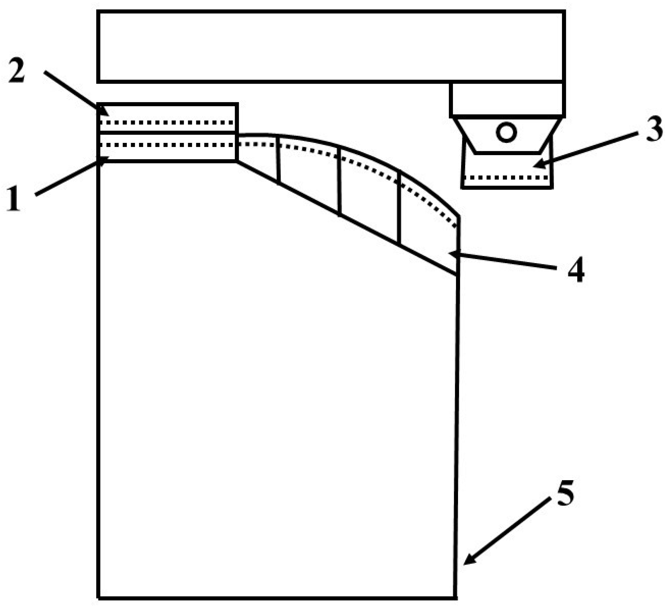
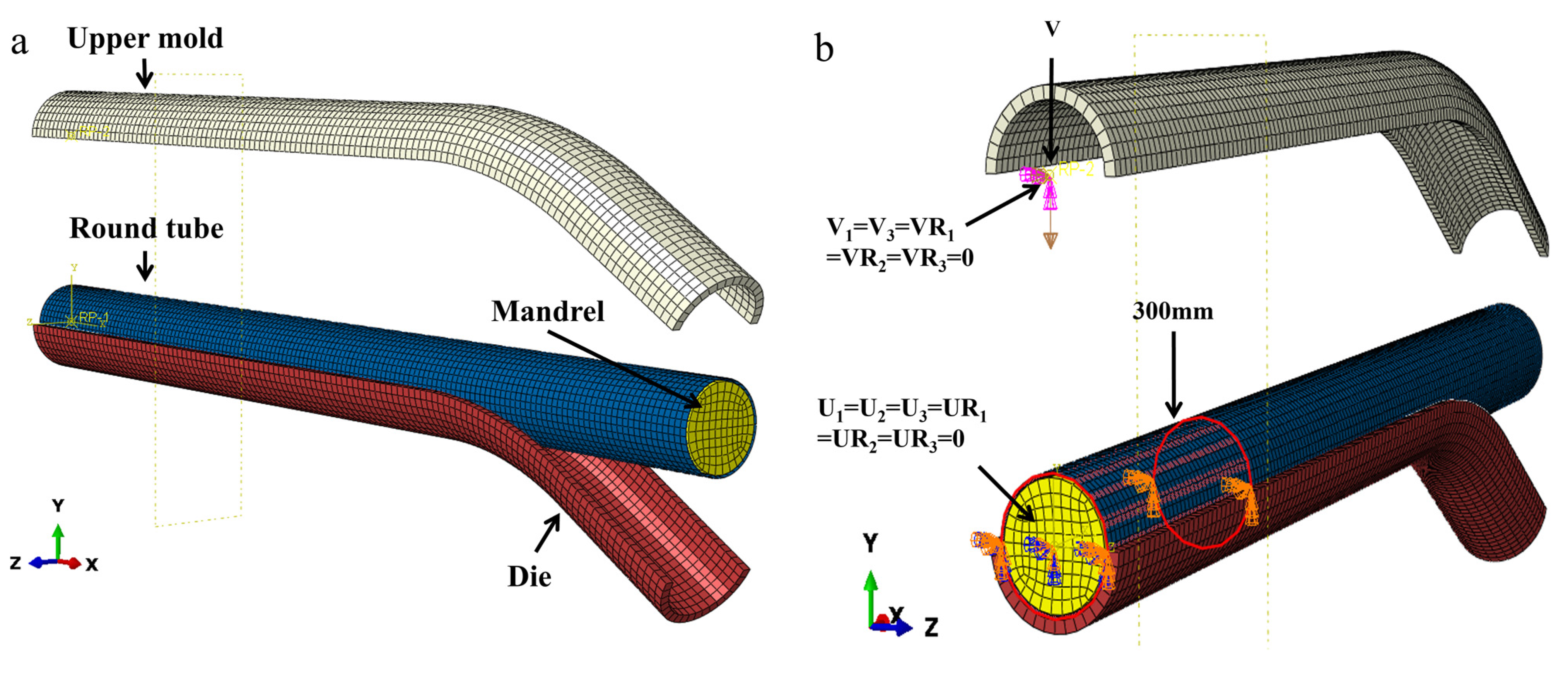
2.2. Finite Element Modeling

This study developed a three-dimensional elastic–plastic finite element model to simulate the pipe bending and springback process of the 7075 aluminum alloy using ABAQUS 2021 software. The model consists of four components: the upper die, lower die, 7075 aluminum alloy pipe, and mandrel. The pipe is modeled as a shell with a thickness of 3 mm using S4R elements.

When setting the grid, the initial grid cell size is 10 mm, and the 7075 pipe network pattern part of the key component with a length of 100 and a wall thickness of 3mm is refined and gradually reduced to 9 mm, 8 mm, 7 mm, and 6 mm, keeping the grid size of the mold and the non-deformation area unchanged. With local mesh refinement, the mesh quality is good, and the change in the wall thickness reduction rate tends to be stable. Taking into account both accuracy and efficiency, the size of the pipe element is finally set to 8mm, and the pipes in each mold and non-deformation area are divided into 10mm by a coarse-grained grid [39].

In regions where deformation is minimal, including the mold areas, a coarser mesh with a cell size of 10 mm is applied. The model includes 26,983 elements and 29,062 nodes, as shown in Figure 2a.

The elastic–plastic deformation characteristics of the 7075 aluminum alloy were determined through unidirectional tensile tests on a batch of the same material. The experimental stress–strain data were converted and imported into the material database of Abaqus. The material parameters are summarized in

Table 2. Material properties of the 7075 aluminum alloy.

Young’s Modulus (Mpa)	Densities (Kg/m3)	Yield Stress	Yield Strain	Poisson’s Ratio
72,000	2180	---	0.2	0.33

. The contact interactions between the pipe and the molds are modeled as face-to-face contact. Normal contact is described using a penalty function to prevent mutual penetration between the deformed pipe and the rigid mold components. Tangential contact is defined as hard contact, and the Coulomb friction model is used to describe the frictional interactions between the contact surfaces as follows:

$$f=\mu \times F_n$$

(1)

where μ = 0.1 is the friction coefficient between the pipe embryo and each mold and F_n is the normal phase pressure at the contact interface.

Considering the complexity of the tube bending and springback process, a dual-algorithm strategy was adopted for the tube pressing–bending and springback process, divided into two analysis steps, to fully leverage the advantages of both algorithms. During the pressing–bending phase, the dynamic explicit algorithm is used to simulate the rapid deformation process of this stage. Specifically, the lower die is fixed while the upper die is given a velocity to simulate the pressing action. After the pressing–bending is completed, the analysis switches to a steady-state analysis. At this point, the system has transitioned from dynamic loading to a relatively stable deformation phase, and steady-state analysis can simulate the springback process more efficiently, ensuring simulation accuracy while significantly reducing computation time. To replicate real-world working conditions, the unbent end of the pipe is fixed with a 300 mm length, and the mandrel is constrained to the same side of the end face to ensure the pipe’s stability during the bending process. The complete loading and boundary conditions are illustrated in Figure 2b.

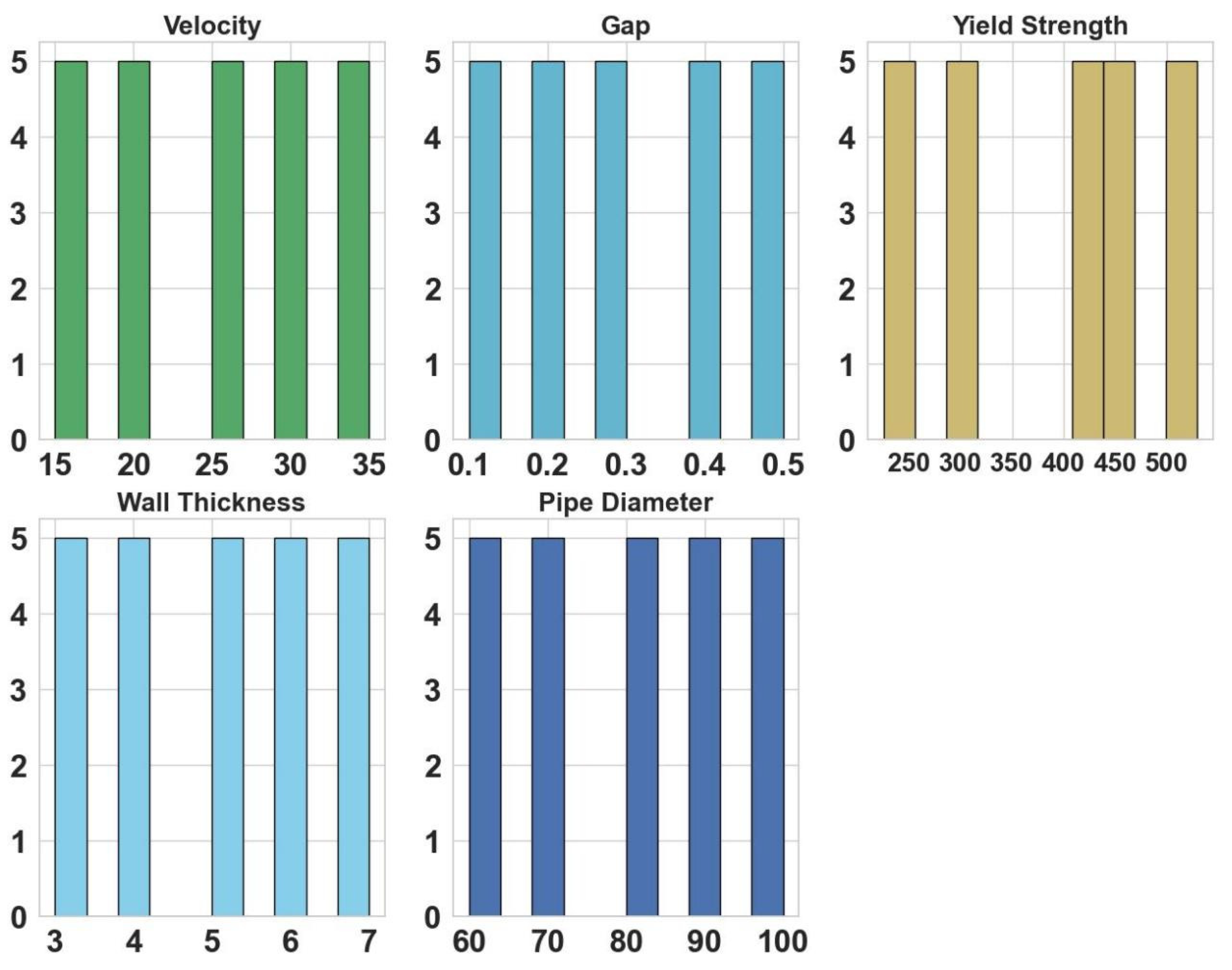
2.3. Orthogonal Experimental Design with Different Process Parameters

Orthogonal tests are widely used in both industrial production and scientific research [40]. Following the principles of orthogonal design, a five-factor, five-level orthogonal experimental design was conducted using the L25 array. The process parameters selected for this study included five material properties, pipe wall thickness, pipe diameter, bending speed, and mandrel-to-pipe clearance. The evaluation indexes were the springback angle, cross-sectional distortion rate, maximum inner wall thickening rate, and maximum outer thinning rate. The factor ranges for each level are specified in

Table 3. Correspondence table of horizontal factors.

Horizontal Factors
	A (Yield Strength)	B (Wall Thickness)	C (Pipe Diameter)	D (Speed)	E (Mandrel–Pipe Clearance)
1	225	3	60	15	0.1
2	293	4	70	20	0.2
3	426	5	80	25	0.3
4	440	6	90	30	0.4
5	530	7	100	35	0.5

. The purpose of the orthogonal test design is to optimize forming quality by analyzing test data, determining the optimal process parameters, and assessing the impact of the selected factors on the forming quality of the pipe fittings, as well as their cross-coupling relationships.

For the material properties, the yield strength of the 7075 aluminum alloy in various heat-treated states was used, as reported by Chen et al. [41] and Feng et al. [42]. The 7075 aluminum alloy was heated to 475 °C and held for 5 min and was then transferred to the die within 5–7 s, followed by die-pressured cooling with a pressure of 5 MPa applied for 10 s to obtain a supersaturated aluminum alloy solid solution. After natural aging for 4 h (this state, referred to as the W state, is the condition of the aluminum alloy immediately after solution heat treatment without significant natural aging), the yield strength was 225 MPa; after natural aging for 48 h, the yield strength of the W state was 293 MPa; after being left at room temperature for 12 h and then aged at 120 °C for 20 h in a single-step aging process, the yield strength reached 530 MPa; and to shorten the aging treatment time, a higher aging temperature was used to promote the precipitation of the second phase, and after short-term aging for 25 min at 200 °C, the yield strength was 440 MPa [31].

Quasi-static tensile tests were conducted at room temperature using an INSTRON 8801 small-load hydraulic fatigue testing machine, with the load measured by the machine’s built-in load sensor. The yield stress was determined as the stress value at a residual strain of 0.2% after unloading, which was 426 MPa [42].

2.4. Prediction Method for Inner Wall Thinning, Outer Wall Thickening, and Springback

In this paper, parameters such as inner wall thinning, outer wall thickening, ellipticity, and springback angle of the pipe during the bending process were predicted using the Abaqus platform. The coordinates of the innermost and outermost nodes of the pipe were analyzed with the coordinate method to accurately calculate various forming defects after bending. First, the pipe was analyzed cross-sectionally, and a section was taken from the part of the pipe where the wall thickness exhibited the most significant change. This section was used to obtain the inner and outer ridges of the pipe. Next, the different locations of the inner and outer rims were labeled, and the coordinates of the nodes at these locations were extracted from Abaqus. The two innermost and outermost nodes in the cross-section were selected, and the distance between them was calculated.

To measure the pipe bending quality and calculate the forming defects, the following quality standard parameters are defined: wall thickness change rate I_t = |t₀ − t₁/t₀| × 100%, where t₀ is the wall thickness at the outer ridge before bending and t₁ is the wall thickness at the outer ridge after bending. The cross-sectional distortion rate is |D_max − D_min/D₀| × 100%, where D₀ is the nominal diameter of the circular pipe and D_max and D_min are the measured maximum and minimum outside diameters of the pipe cross-section, respectively. The springback of a pipe after forming is generally referred to as the angle of springback (Δa = Δa₀ − Δa₁), which is used to calculate the difference between the actual angle after bending and the ideal angle to assess the forming accuracy.

2.5. Transfer Learning

Transfer learning addresses the problem of biased model results by transferring the parameters of a pre-trained model to a new model, thereby helping to train the new model more effectively. Since most data or tasks are related, the knowledge acquired by the pre-trained model can be leveraged by the new model through transfer learning, thereby improving learning efficiency and accelerating the training process.

In transfer learning, the existing knowledge was referred to as the ‘source domain’, while the new knowledge to be learned was called the ‘target domain’ [43]. The goal of transfer learning was to transfer knowledge from the source domain to the target domain. By leveraging existing knowledge to solve problems in different but related domains, transfer learning relaxed the basic assumptions of traditional machine learning—such as sample independence and homogeneous data distribution. Its goal was to apply knowledge from the source domain to address learning problems in the target domain, often with only a small amount of labeled data or even none.

There is a source task and a target task. Let the source task dataset be $Ds={\{(x_i^S,y_i^S)\}}_{i=1}^{n_S}$ and the target task dataset be $D_T={\{(x_i^T,y_i^T)\}}_{i=1}^{n_T}$, where $x$_i represents the input features, $y$_i represents the labels, and n_S and n_T are the number of samples in the source and target datasets, respectively. The source task learning objective is typically used to minimize the loss function over the source domain as follows:

$$L_S\left(\theta \right)={\displaystyle \frac{1}{n_S}}{\sum }_{i=1}^{n_S}L(f(x_i^S;\theta ),y_i^S)$$

(2)

where $f$($x$;$\theta$) is the model’s prediction for the source task, L is the loss function, and $\theta$ represents the model parameters. The goal of transfer learning is to improve performance on the target task by leveraging the knowledge from the source task. Transfer learning is actually used to continue training the model on the target task, which is trained on the source task. Thus, the loss function of the target task is calculated on the basis of the source task. The target task loss function is defined as follows:

$$L_T\left(\theta \right)={\displaystyle \frac{1}{n_T}}{\sum }_{i=1}^{n_T}L(f({\sum }_{i=1}^{n_S}L(f(x_i^T;\theta ),y_i^T)$$

(3)

In transfer learning, we typically minimize the target task loss while incorporating the source task knowledge. This can be performed by regularizing the target task’s loss function, typically in the following form:

$$L_T\left(\theta \right)=L_T\left(\theta \right)+\lambda \times R(\theta )$$

(4)

where λ is the regularization parameter and R($\theta$) represents the regularization term, which adjusts the model based on the source task knowledge.

3. Results and Discussion

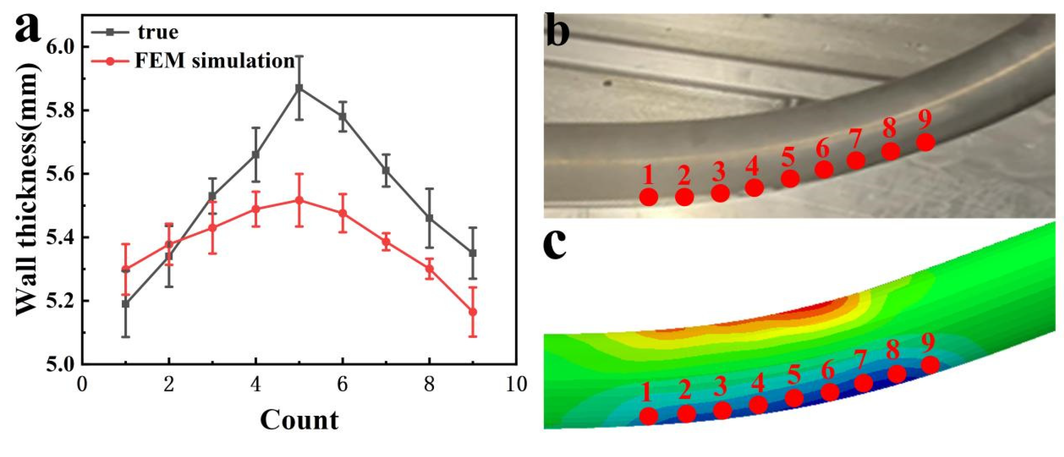
3.1. Experimental Results

During the press bending experiments on a 7075 aluminum alloy tube (Institute of Metal Research, Chinese Academy of Sciences, Shenyang, China) with an outer diameter of 1000 mm and a wall thickness of 3 mm, the total length of the bent region was measured starting from the tangent point between the tube and the bending die, resulting in a length of 270 mm. Marks were made at 30 mm intervals along the arc segment of the tube, and the variations in wall thickness at the nine marked points within the bent region were measured. The experimentally measured values were compared with the corresponding Abaqus simulation results, as shown in Figure 3. The average of the nine measured values was 5.532, showing only a 2.7% error compared to the simulated value average of 5.382.

In this study, a bending experiment was also conducted on 7075 aluminum alloy pipes with an outer diameter of 1000 mm and wall thicknesses of 3 mm, 4 mm, 5 mm, 6 mm, 7 mm, and 8 mm, respectively. The springback angle was measured both before and after bending. The experimental results were then compared with the simulation results obtained using Abaqus, as shown in Figure 4. The average springback angle measured experimentally was 2.316, while the average value obtained from the Abaqus simulation was 2.448. The error between the experimental and simulation results was only 5.6%.

3.2. Results of Finite Element Simulation Orthogonal Test Data

Table 3 shows the results of the orthogonal test of the springback angle and the analysis of the orthogonal results. In the intuitive analysis method, the five different factors are judged by the extreme difference R. The larger value of R indicates that the factors affect the results to a greater extent. k represents the degree of influence of each level on the evaluation index of the test, and it is used to analyze the optimal combination scheme among the horizontal factor levels. From the data in the table, it can be seen that the factors affect the springback angle in the following order of precedence: A (material properties) > C (pipe diameter)> E (clearance) > B (wall thickness) > D (speed). Based on the results of the analysis, the optimum horizontal factor combination of the factors affecting the springback angle is derived as A1C5E4B1D1. That is, the material properties are the yield strength 225 MPa of the 7075 aluminum alloy pipe in the W state obtained under the condition of heating at 475 °C for 5 min; the diameter of the pipe is 60 mm, the clearance between the mandrel and the pipe is 0.4 mm, the wall thickness is 3 mm, and the speed is 30 mm/s. The trend curves of the springback angle, cross-section distortion rate, outer wall thinning rate, and inner wall thickening rate under different parameter combinations in orthogonal tests are shown in Figure 5. According to the steepness and flatness of the curve, it can be more intuitive to determine the primary and secondary factors, as well as the change in the factor indicators of the changes in their bending and forming law.

In Figure 5a, it can be concluded that the key factors influencing the springback angle align with the ANOVA results presented in

Table 4. Analysis table of springback angle results.

	A	B	C	D	E
K1	10.09	16.44	24.46	15.94	18.99
K2	12.14	18.16	20.49	18.36	19.68
K3	20.54	17.65	18.12	18.5	17.17
K4	21.86	20.15	14.79	19.41	15.84
K5	26.83	19.06	13.6	19.25	19.78
K1	2.01	3.28	4.89	3.18	3.79
K2	2.42	3.632	4.09	3.672	3.93
K3	4.1	3.53	3.62	3.7	3.43
K4	4.372	4.03	2.95	3.88	3.16
K5	5.36	3.812	2.72	3.85	3.95
R1	3.34	0.742	2.172	0.69	0.78

. The material property (A), specifically the yield strength at different heat-treated states, has the most significant effect on the springback angle compared to other factors. As the yield strength increases, the springback angle increases substantially, with a steep trend plot, indicating that material properties are the primary factor affecting the springback angle, which is consistent with the ANOVA findings. In contrast, the pipe diameter (C) exhibits a decreasing effect on the springback angle. As the diameter increases, the springback angle gradually decreases, and the trend plot is similarly steep, reflecting a significant influence. However, the factors of wall thickness (B), speed (D), and mandrel-to-pipe clearance (E) have a lesser impact on the springback angle, with relatively smaller changes and flatter trend plots. This can be attributed to the fact that these factors interact with other process parameters, and their combined effect is more influential than the impact of any single factor alone. In Figure 5b, the trend of the cross-sectional distortion rate differs from that of the springback angle. The data indicate that the pipe diameter (C) significantly affects the cross-sectional distortion rate. As the pipe diameter increases, the cross-sectional distortion rate decreases substantially, with a larger reduction observed. This can be attributed to the fact that larger pipe diameters better distribute the bending stresses, reducing the amount of cross-sectional distortion. Additionally, the mandrel-to-pipe clearance (E) plays a crucial role in influencing the cross-sectional distortion rate. As the gap increases, the cross-sectional distortion rate increases because a larger gap results in insufficient support from the mandrel, making the pipe’s cross-section more susceptible to deformation during the external bending process. The effect of speed (D) on the cross-sectional distortion rate is relatively less pronounced compared to other factors, although there is a slight trend observed. As the bending speed increases, the cross-sectional distortion rate marginally increases. This can be attributed to the fact that higher speeds may lead to more abrupt deformation, resulting in higher internal stresses that cause slight distortion of the pipe’s cross-section. However, this effect is less significant than the influence of pipe diameter (C) or mandrel-to-pipe clearance (E). The trend plots for the inner wall thickening rate (c) and outer wall thinning rate (d) shown in Figure 5c,d are similar.

In summary, the results highlight that the yield strength of the material and the pipe diameter are the most influential factors in determining the springback angle and cross-sectional distortion rate, while other factors such as wall thickness, bending speed, and mandrel-to-pipe clearance have a more subtle impact. These findings provide valuable insights into the optimization of the bending process, suggesting that controlling material properties and pipe geometry is key to minimizing forming defects, like springback and cross-sectional distortion.

3.3. Machine Learning to Predict Springback Angle

3.3.1. Dataset Description

The dataset is the result generated by finite element simulation, which is the same as the dataset used in the orthogonal test analysis in the previous paper, and the dataset is divided into two parts: the training set and the test set. The training set consists of 25 samples generated by orthogonal tests, and the test set consists of 60 samples generated by random sampling, with five key features recorded in each sample set: yield strength, wall thickness, pipe diameter, speed, and clearance; three intermediate test results: distortion rate, thickening rate, and thinning rate; and the final prediction of the target bending springback angle of the test for the 7075 aluminum alloy pipe. After the orthogonal test screening, each feature covered different values and was evenly distributed, and the sample size is shown in Figure 6. In the twenty-five samples, each feature has five different values, and there are five samples for each value, so the distribution of all features is uniform. The feature correlation matrix is shown in Figure 7. In the figure, it can be seen that the springback angle has a strong positive correlation with the yield strength and a more obvious negative correlation with the pipe diameter, and the remaining three features have a relatively low correlation with the springback angle. In addition, according to the feature correlation matrix, it can be seen that the correlation between two features is close to 0 or equal to 0, which can show that the orthogonal test is effective for screening the values of the features. Figure 8 shows the distribution of springback angle values, and Figure 9 shows a schematic diagram of the springback angle distribution, where the dark blue area is the kernel function density curve, cyan is the sample distribution frequency histogram, and orange is the mean value. The figure shows that the distribution of the range of values of the springback angle in the training set is relatively uniform, which can cover most of the cases of the springback angle. In Figure 9, it can be seen that the distribution of the springback angle is different between the training set and the test set, which can also better validate the performance of the model as well as its generalization ability and test whether the model is biased in the fitting process.

3.3.2. Data Preprocessing

Data preprocessing is an essential step before training an ML model. The variables in the model should be classified as independent and dependent variables. In our dataset, yield strength, wall thickness, pipe diameter, velocity, and clearance were defined as the independent variables of the ML model. In contrast, the rebound angle was defined as the dependent variable and the ML model’s output. The result of the experimental test was confirmed successful (accept) if it conformed to the predetermined dimensions; all other test results were confirmed unsuccessful (reject). These were saved in an Excel file and transferred to the DataFrame variables of the Pandas library. The independent variables were assigned to x and the dependent variable to y. The datasets generated by the orthogonal test are used as the training datasets (training set), and the other 60 samples were used in testing the models (testing set). Consequently, the training set is used to train the model to learn the behaviors present in the training data, and the testing set is used to test the model’s accuracy. The independent variable’s training data and test data were assigned to the X train and X test variables, respectively, and the dependent variable’s training data and test data were assigned to the y train and Y test variables, respectively. To standardize the dataset, the ‘StandardScaler’ function was imported from the scikitlearn library and employed; hence, the data preprocessing step was completed by converting the X train variable to the X train variable and the X test variable to the X test variable. The preprocessing was finished. In deep learning, the number of samples is sufficient; the more samples there are, the better the effect of the trained model will be and the stronger the model’s generalization ability. However, in practice, the number of samples is insufficient, or the quality is not good enough. When the training data is insufficient, the model may learn the noise in the data instead of the underlying data distribution, resulting in overfitting. Then, data augmentation is necessary to improve the quality of the samples. Data augmentation is a technique to artificially increase the training set by creating a modified copy of the dataset using existing data, and it is one of the commonly used techniques in deep learning that involves making small changes to the dataset or using deep learning to generate new data points. Data augmentation is mainly used to increase the training dataset to make the dataset as diverse as possible, making the trained model more generalizable. Data augmentation reduces this risk by increasing the diversity of the data. Enhanced data can cover more input space, improve model generalization ability, and make the model performance more stable in the face of new data. Data enhancement can be categorized into supervised and unsupervised data enhancement methods. Supervised data enhancement can be divided into single- and multi-sample data enhancement methods. In contrast, unsupervised data enhancement can be divided into generating new data and learning enhancement strategies.

In this experiment, since the training set of the finite element test obtained from the orthogonal test has only 25 samples, an unsupervised data enhancement method is used to generate new samples by averaging the eigenvalues of the different samples. According to the empirical values set, the sample number is randomly generated between 2 and 5; each time, the non-return sampling takes the average value as the new sample after taking a random number of samples. Since there are 60 samples in the test set and 25 samples in the training set, 35 fusion samples are generated by data enhancement. The distribution of the springback angle after data enhancement is shown in Figure 10. The enhanced data increases the distribution of the springback angle between 3 and 5, which enriches the input spatial distribution of the training set and improves the generalization of the dataset.

3.3.3. Evaluation Functions

In the performance evaluation of regression models, the mean absolute error (MAE), mean square error (MSE), mean absolute percentage error (MAPE), and coefficient of determination (R²) are the core evaluation functions, quantifying the deviation between the predicted value and the true value and the explanatory ability of the model from different perspectives.

The MAE is defined as the mean of the absolute deviation between the predicted value and the true value, and its mathematical expression is as follows.

$$MAE={\displaystyle \frac{1}{n}}\sum _{i=1}^n|y_i-{\widehat{y}}_i|$$

The MAE directly reflects the absolute magnitude of prediction errors, is insensitive to outliers, and is suitable for scenarios that need to equalize the effect of errors, such as engineering forecasting with high robustness requirements. Its numerical range is nonnegative real numbers, and smaller values indicate higher prediction accuracy of the model.

The MSE amplifies the influence of large errors through square operation, and the calculation formula is as follows:

$$MSE={\displaystyle \frac{1}{n}}\sum _{i=1}^n{(y_i-{\widehat{y}}_i)}^2$$

The MSE is sensitive to outliers and is often used in gradient descent optimization where derivable loss functions are required (e.g., linear regression models).

The MAPE measures the relative error in percentage terms and is as follows:

$$MAPE={\displaystyle \frac{100\%}{n}}\sum _{t=1}^n\left|{\displaystyle \frac{y_i-{\widehat{y}}_i}{y_i}}\right|$$

The MAPE is useful for horizontal comparisons of data at different dimensions, but it is sensitive to true values near zero (the denominators diverge as they approach zero). The lower its value, the better model prediction consistency.

R² represents the ability of the model to explain the variance of the target variable. The formula is as follows:

$$R^2=1-{\displaystyle \frac{{\sum }_{i=1}^n{(y_i-{\widehat{y}}_i)}^2}{{\sum }_{i=1}^n{(y_i-{\overline{y}}_i)}^2}}$$

The R² range is [0, 1], and the closer to 1, the better the model fit.

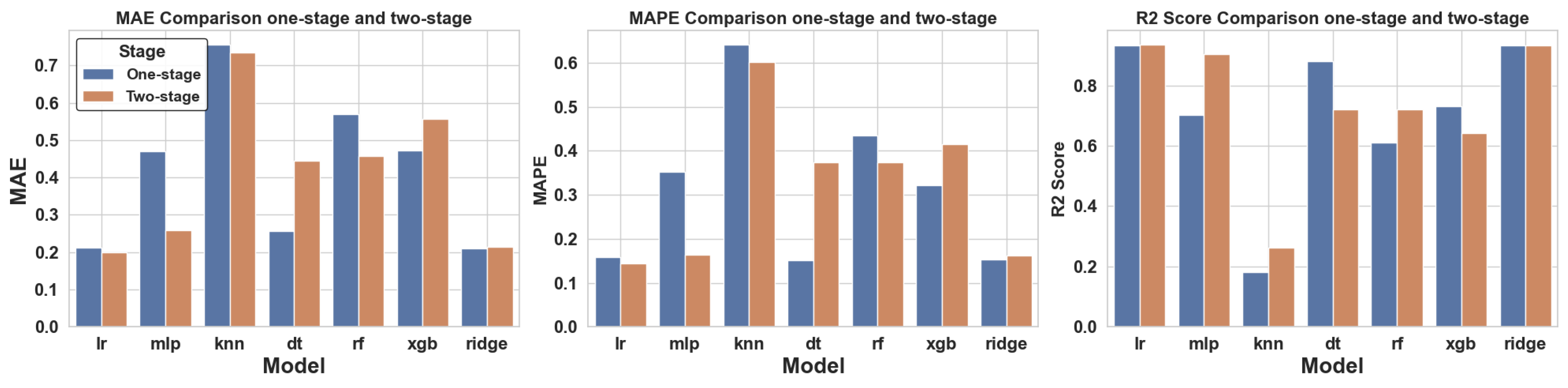
3.3.4. Multi-Stage Forecasting

Multi-stage forecasting is a hierarchical step-by-step approach to forecasting and is shown schematically in Figure 11. It approaches the final prediction goal gradually through multiple stages of prediction, each using the previous stage’s output as input. This method is often used to deal with complex problems, especially when it is difficult to predict the final goal directly or when there is a hierarchical relationship between the data. This approach allows the complex prediction task to be broken down into multiple smaller, relatively independent prediction tasks, with each stage focusing on predicting an intermediate variable or feature. Each stage can use a different model and feature set to gradually improve the accuracy of the final target’s prediction. In this paper’s 7075 aluminum alloy pipe bending springback scenario, the cross-section distortion rate, thickening rate, and thinning rate are key factors that directly affect the forming quality. By accurately predicting these parameters, the springback angle can be predicted and controlled more effectively, so the task of predicting the springback angle can be decomposed into two parts. The first part of the task predicts the intermediate indexes of the distortion rate, thickening rate, and thinning rate, and the second phase of the task combines the three intermediate indexes obtained by prediction and jointly predicts the final prediction target springback angle.

3.3.5. Multi-Stage Prediction Results

All the default parameters are used for the first stage prediction. It can be seen that linear regression has the best-fitting effect, and the comparison between the predicted values and the true values in the specific test set is shown in Figure 12, where the horizontal coordinates represent the samples. The vertical coordinates represent the springback angle. The distribution of the predicted and true values in the test set is very close to each other, and there is no large deviation, indicating that the linear regression model has the best-fitting effect on this dataset. The importance of the features obtained from the coefficients of the corresponding features of the linear regression model is shown in Figure 13. The material properties and pipe diameter have the greatest impact on the accuracy of predicting the springback angle, which is 51.1% and 31.6%, respectively, and this is consistent with the results in the feature correlation analysis. Since the cross-section distortion rate, thickening rate, thinning rate, and other indicators are indicators that will continue to change with the bending process of the 7075 aluminum alloy pipe, which has a certain correlation with the change in the springback angle, the task of predicting the springback angle is divided into a two-stage task. In the first stage, the intermediate variables are predicted first. The predicted intermediate variables with the input features are fed into the prediction model in the second stage, and finally, the springback angle is predicted. In the second-stage prediction model, the input features of the first-stage model are the same as those in the first-stage prediction. The gap, wall thickness, speed, pipe diameter, and yield strength features are inputted. Still, the first-stage model’s prediction target differs from the first-stage prediction. The prediction target is the distortion rate, the thickening rate, and the thinning rate, which directly affect the springback angle, i.e., the input dimension is 5 and the output dimension is 3. After the prediction is obtained, the distortion rate, thickening rate, and thinning rate are combined with the five features inputted from the first-stage prediction model into the second-stage prediction model, and the prediction target is the springback angle, i.e., the input dimension is 8 and the output dimension is 1. The task of springback angle prediction is split into two subtasks using multi-stage prediction. Task one is to predict the distortion, thickening, and thinning rates by inputting the gap, wall thickness, speed, tube diameter, and yield strength. Task two is to input the input gap, wall thickness, speed, pipe diameter, yield strength distortion rate, thickening rate, and thinning rate and predict the springback angle, and the result is shown in

Table 5. Table of the springback angle prediction results for each model for one stage and second stage.

Method	First Stage			Second Stage
	MAE	MAPE	R2	MAE	MAPE	R2
Linear regression	0.2876	0.4623	0.1876	0.1992	0.1444	0.9343
Ridge regression	0.2838	0.4261	0.1348	0.2141	0.1625	0.9316
Multilayer perceptrons	0.4112	0.3965	−0.1598	0.2579	0.1644	0.9046
K-nearest neighbor	0.7438	0.7423	−1.6376	0.7353	0.6016	0.2617
Decision tree	0.3134	0.318	0.2134	0.2378	0.14	0.8537
Random forest	0.3126	0.5211	0.3151	0.4409	0.3515	0.7478
XGBoost	0.4317	0.6768	−0.338	0.5576	0.4147	0.6422

.

Since SVM and LGBM do not support multi-objective regression, second-stage prediction experiments were not performed. The comparative effect of the experimental metrics is shown in Figure 14. As can be seen in the figure, by splitting the subtask of springback angle prediction into a two-stage prediction task, in addition to the decision tree and XGBoost, all the indicators of the remaining machine learning models have a certain degree of improvement, of which the multilayer perceptual machine and the random forest are the most obvious, and the best-performing linear regression also has a small increase in the performance, which proves that this subtask-splitting method has a significant effect on the improvement of performance. Since there is no tunable parameter for linear regression, the optimization is performed for the ridge regression method with the L2 regularization term added to linear regression. The L2 regularization coefficients are 0.01, 0.02, 0.05, 0.08, 0.1,0.15, 0.2, 0.3, 0.5, 0.8, 1, 2, 5, 10, 20, 30, 40, and 50. The Solver is taken as ‘svd’, ‘cholesky’, ‘saga’, ‘sparse-cg’, ‘lsqr’, and ‘auto’, and the experimental results are shown in Figure 15. In the figure, the X-axis is the L2 regularization coefficient, the solid part of the curve is the average value, and the upper and lower bounds are the maximum and minimum values when the Solver takes different values, respectively. As can be seen in the figure, the optimal regularization coefficient is alpha = 10 when the scores of three evaluation indexes, the MAE, MAPE, and R², are all optimal, where alpha = 10, MAE = 0.1499, MAPE = 0.0991, and R² = 0.9669. Compared with the results of the default value before tuning, the MAE improved by 30%, the MAPE enhanced by 39%, and the R² improved by 3.79%, and it can be seen that parameter tuning has produced a significant enhancement of the model performance.

3.4. Experiments on Real Collection Data

The experimental results in this section are all modeled based on finite element simulation data and have not been verified in real experimental scenarios. Therefore, in this section, experiments will be conducted on the dataset consisting of the collected real circular pipe bending springback data to verify further the practical value of the method proposed in this paper in real circular pipe bending scenarios.

3.4.1. Prediction of the Real Dataset Based on Transfer Learning

This paper uses transfer learning to validate the experimental data collected in real scenarios experimentally. The two-stage prediction method in Section 3.4 has significantly improved the prediction accuracy, so the experiments in this section of the validation experiments are conducted based on the two-stage method. The real collection dataset is collected by first determining the pipe diameter, speed, gap, yield strength, and wall thickness parameters, and then bending experiments are carried out on round pipes of the corresponding materials using a press machine. The parameters of the bent round pipes are measured to calculate the distortion rate, the thickening rate, the thinning rate, and the springback angle. The parameter settings refer to common parameters in actual production scenarios, totaling 30 datasets. The specific application of transfer learning lies in the fact that the simulation dataset obtained from finite element simulation is first utilized as the source domain training set to train the two-stage prediction model, and the specific setup is the same as the experimental setup in Section 3.4. Then, the real dataset is divided; 60% is selected as the target domain training set, and the remaining 40% is used as the test set for transfer learning. After the model training results are based on the source domain dataset, the model continues to be trained to fit the target domain training set, and the transfer learning test set is utilized to verify the model learning effect.

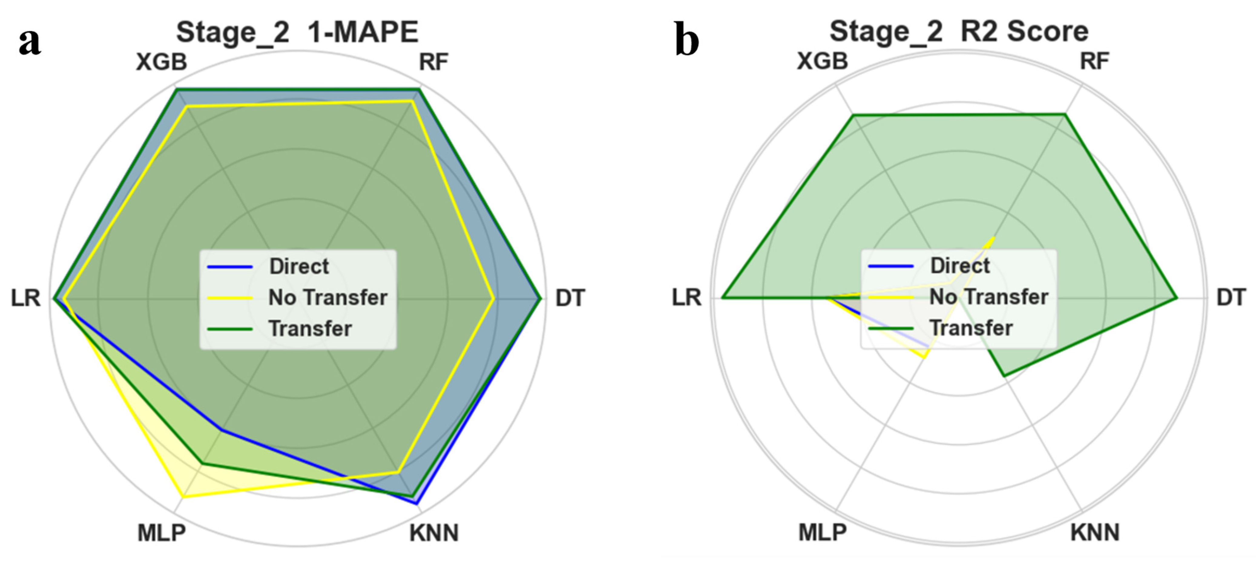
3.4.2. Transfer Learning Results

To demonstrate the effectiveness of transfer learning, three groups of experiments were conducted for comparison. The first two groups serve as control groups, where transfer learning is not applied, while the third group employs transfer learning. In the first group, the two-stage model is trained on the source domain training set, and the source domain model is directly used to predict the target domain test set. In the second group, the two-stage model is trained on the target domain training set and tested on the target domain test set. In the third group, transfer learning is applied. The two-stage model is first trained on the source domain training set and fine tuned on the target domain training set, followed by testing on the target domain test set. The experimental results are summarized in

Table 6. Results comparison.

Method	Direct			Learning Without Transfer			Transfer Learning
	MAE	MAPE	R2	MAE	MAPE	R2	MAE	MAPE	R2
Decision Tree	0.7993	0.1918	−5.7497	0.1252	0.032	0.7769	0.1168	0.0299	0.797
Random Forest	0.3842	0.0928	−0.5039	0.1287	0.0333	0.7619	0.1234	0.0318	0.7644
XGB	0.467	0.1099	−1.7342	0.1256	0.0318	0.7672	0.1256	0.0318	0.7672
Linear Regression	0.2555	0.0628	0.2994	0.0948	0.0249	0.8791	0.0941	0.0247	0.8804
MLP	0.3375	0.0848	−0.5363	1.7704	0.4867	−112.11	1.0447	0.2716	−11.72
K-Nearest Neighbors	0.8229	0.1959	−6.8323	0.1925	0.0496	0.5573	0.3227	0.0837	−0.0808

.

To visualize the performance improvement achieved by transfer learning, the results are presented as radar charts in Figure 16a,b. For clarity, the MAPE is converted to 1-MAPE, representing the proximity to the true value. Since the MAE and MAPE are highly correlated, only the MAPE and R² results are shown. In order to show the effectiveness of the proposed method, we also compare the results in other papers on rebound angle prediction models, as shown in

Table 7. Results comparison with other methods.

Method	MAE	MAPE
NMLPR [31]	6.4512	0.0645
ANN [44]	/	0.0880
Analytical model [45]	/	0.0374
Our method	0.0941	0.0247

. Since the evaluation metrics adopted by each paper are different, only their corresponding metrics are shown. As can be seen in the table, the proposed method is significantly better than the methods in other papers, and the performance of rebound angle prediction is significantly improved.

The error analysis between the true rebound angle and the predicted value is shown in Figure 17. The ordinate represents the number of samples corresponding to the rebound value, and the upper and lower black horizontal lines represent the maximum and minimum values of the distribution of sample values predicted by the model in the process of repeating five random trials. It can be seen that the region with a small springback angle fluctuates to some extent with the distribution difference of the true sample, while in the region with a large rebound angle, the distribution is relatively stable with only a few prediction error distributions. Therefore, there is uncertainty in the prediction of the proposed model when the springback angle is small, but the uncertainty and prediction error are both low in the part of the springback angle greater than 3 degrees.

The results indicate that except for the MLP model, the performance of all other models improved significantly with transfer learning. In contrast, the performance without transfer learning is almost identical to that of direct prediction, suggesting that the distribution of the finite element simulation results and real experimental data are relatively similar. Transfer learning outperforms the other two methods, likely due to the small sample size and distribution bias of the real experimental dataset. When training directly on real samples, the larger distribution gap between the training and test sets results in poorer performance. However, pre-training on the simulated dataset effectively expands the training set, improving model performance. This confirms that the transfer learning approach proposed in this study is effective.

4. Conclusions

In this study, a method combining Abaqus FEM and nonlinear machine learning is proposed to effectively predict the bending springback angle of 7075 aluminum alloy pipes. Five key factors, namely, material properties (yield strength at different heat treatment states), wall thickness, tube diameter, speed, and mandrel–tube gap, were analyzed to predict the springback angle accurately, and the main conclusions are as follows:

• Based on the entropy value method polar analysis and ANOVA on the comprehensive score of bending and forming defects, it is unanimously pointed out that the pipe diameter is the most significant influencing factor. The intuitive analysis of the single index springback angle shows that the material properties and pipe diameter have a significant effect, proving that orthogonal test eigenvalue screening is effective. It further verifies that the springback angle of large pipe diameter bending and forming has high research value.
• Using data enhancement techniques based on small samples greatly reduces the time required to collect simulation experimental samples. It avoids the finite element simulation for the high dependence on technical reserves, as well as in the large-scale or high complexity of the simulation of the computational inefficiency problem. Through the data enhancement technique, the distribution interval of the sample variables is greatly expanded, and the diversity of the samples is increased, which effectively improves the model’s ability to deal with small sample data and the model’s generalization ability.
• A multi-stage prediction model based on ridge regression is established and compared with common machine learning models, and the R2 correlation score on the final test set reaches 0.9669, which shows the higher prediction accuracy of the model and the universality of the prediction of pipe bending springback. The model can be integrated into a real pipe bending production system and trained using real-time production data, providing strong technical support for accurately forming high-strength aluminum alloy pipes.
• Analogous to the transfer learning pre-training approach, it takes the first pre-training on the simulated dataset. Subsequently, the pre-trained two-stage prediction model is trained on the experimental dataset for transfer learning. Compared with the two methods of direct prediction after training on the simulated dataset and direct training of prediction on the experimental dataset, the transfer learning approach achieves a more significant prediction accuracy.
• Due to the small amount of data that can be collected in the real production environment, there is a certain deviation between the data obtained by finite element simulation and the feedback of the real scene. The multi-stage prediction and transfer learning prediction methods proposed in this paper use simulation data for model pre-training and fine tuning and multi-stage prediction on real data, which can effectively reduce the impact of the deviation between simulation data and real data and significantly improve the prediction accuracy of the rebound angle in real production scenarios.

References

1. Yang, J.; Zhan, Y.; Hon, G.B. Current Status and Development Plan of Military Helicopter Equipment in the World. Helicopter Tech. 2020, 3, 68–72. [Google Scholar]
2. Canumalla, R.; Jayaraman, T.V. Decision science-driven assessment of Ti alloys for aircraft landing gear beams. Aerospace 2024, 11, 51. [Google Scholar] [CrossRef]
3. Liang, T.; Yin, Y.; Yin, Q.; Nie, H.; Wei, X. Comparative research on landing and rollout characteristics of skid-equipped and wheeled aircraft. J. Aircr. 2025, 62, 34–47. [Google Scholar] [CrossRef]
4. Taskesen, A.; Aksöz, S.; Özdemir, A.T. The effect of cryogenic treatment on ageing behaviour of B4C reinforced 7075 aluminium composites. Met. Mater. 2017, 55, 57–67. [Google Scholar] [CrossRef]
5. Vikas, P.; Sudhakar, I.; MohanaRao, G.; Srinivas, B. Aging behaviour of hot deformed AA7075 aluminium alloy. Mater. Today Proc. 2020, 41, 1013–1017. [Google Scholar] [CrossRef]
6. Aksöz, S.; Kaner, S.; Kaplan, Y. Tribological and aging behavior of hybrid Al 7075 composite reinforced with B4C, SiC, and TiB2. Sci. Sinter. 2021, 53, 311–321. [Google Scholar] [CrossRef]
7. Kang, H.; Zhang, Y.; Zhang, N.; Wang, K.; Du, J.; Ma, K. Microstructure and Mechanical Properties of 7075 Al Alloy TIG-Welded Joint with 7075 Al Alloy Wire as Filler. Trans. Indian Inst. Met. 2024, 77, 2593–2599. [Google Scholar] [CrossRef]
8. Zheng, K.; Dong, Y.; Zheng, D.; Lin, J.; Dean, T.A. An experimental investigation on the deformation and post-formed strength of heat-treatable aluminium alloys using different elevated temperature forming processes. J. Mech. Work. Technol. 2018, 268, 87–96. [Google Scholar] [CrossRef]
9. Zheng, K.; Politis, D.J.; Wang, L.; Lin, J. A review on forming techniques for manufacturing lightweight complex—Shaped aluminium panel components. Int. J. Lightweight Mater. Manuf. 2018, 1, 55–80. [Google Scholar] [CrossRef]
10. Lee, M.S.; Jin, C.K. Investigation of optimal solid solution heat treatment temperature and artificial aging time of Al7075 sheet. J. Mech. Sci. Technol. 2022, 36, 1783–1788. [Google Scholar] [CrossRef]
11. Du, Z.; Han, Y.; Han, D.; Zhang, H.; Mao, X.; Zhang, Z.; Cui, X. Effect of heat treatment and electromagnetic forming on springback and related properties of 7075 aluminum alloy sheet. J. Braz. Soc. Mech. Sci. Eng. 2024, 46, 707. [Google Scholar] [CrossRef]
12. Zhang, Z.; Yu, J.; He, D. Effects of contact body temperature and holding time on the microstructure and mechanical properties of 7075 aluminum alloy in contact solid solution treatment. J. Alloy. Compd. 2020, 823, 153919. [Google Scholar] [CrossRef]
13. Liu, Q.; Chen, S.C.; Gu, R.Y.; Wang, W.R.; Wei, X.C. Effect of heat treatment conditions on mechanical properties and precipitates in sheet metal hot stamping of 7075 aluminum alloy. J. Mater. Eng. Perform. 2018, 27, 4423–4436. [Google Scholar]
14. Kumar, M. AW-7075-T6 sheet for shock heat treatment forming process. Trans. Nonferrous Met. Soc. China 2017, 27, 2156–2162. [Google Scholar] [CrossRef]
15. He, Y.; Li, H.; Zhiyong, Z.; Zhan, M.; Liu, J.; Li, G. Advances and trends on tube bending forming technologies. Chin. J. Aeronaut. 2012, 25, 1–12. [Google Scholar]
16. Dakhore, M.; Kale, A. An overview of pipe bending methods and defects produced for the development of an improved pipe bending mechanism. Adv. Mater. Process. Technol. 2023, 10, 3393–3410. [Google Scholar]
17. Tronvoll, S.A.; Ma, J.; Welo, T. Deformation behavior in tube bending: A comparative study of compression bending and rotary draw bending. Int. J. Adv. Manuf. Technol. 2022, 124, 801–816. [Google Scholar]
18. Wenpei, Z.; Zhili, H.; Huanhuan, L.; Lin, H. Experimental and Numerical Investigation on Springback of Automotive Aluminum Alloy Sheet. Rare Met. Mater. Eng. 2019, 48, 2130–2137. [Google Scholar]
19. Wang, Z.; Lin, Y.; Qiu, L.; Zhang, S.; Fang, D.; He, C.; Wang, L. Spatial variable curvature metallic tube bending springback numerical approximation prediction and compensation method considering cross-section distortion defect. Int. J. Adv. Manuf. Technol. 2021, 118, 1811–1827. [Google Scholar]
20. Sun, C.; Wang, Z.; Zhang, S.; Liu, X.; Wang, L.; Tan, J. Toward axial accuracy prediction and optimization of metal tube bending forming: A novel gru-integrated pb-nsgaiii optimization framework. Eng. Appl. Artif. Intell. 2022, 114, 105193. [Google Scholar]
21. Lee, H.-S.; Park, S.-G.; Hong, M.-P.; Kim, Y.-S. Process design of multi-stage cold forging with small size for ESC solenoid valve parts. J. Mech. Sci. Technol. 2022, 36, 359–370. [Google Scholar] [CrossRef]
22. Ghobadnam, M.; Mosaddegh, P.; Rezaei Rejani, M.; Amirabadi, H.; Ghaei, A. Numerical and experimental analysis of hips sheets in thermoforming process. Int. J. Adv. Manuf. Technol. 2015, 76, 1079–1089. [Google Scholar] [CrossRef]
23. Bock, F.E.; Aydin, R.C.; Cyron, C.J.; Huber, N.; Kalidindi, S.R.; Klusemann, B. A review of the application of machine learning and data mining approaches in continuum materials mechanics. Front. Mater. 2019, 6, 110. [Google Scholar] [CrossRef]
24. Guo, K.; Yang, Z.; Yu, C.-H.; Buehler, M.J. Artificial intelligence and machine learning in design of mechanical materials. Mater. Horizons 2021, 8, 1153–1172. [Google Scholar] [CrossRef] [PubMed]
25. Guo, Z.; Bai, R.; Lei, Z.; Jiang, H.; Liu, D.; Zou, J.; Yan, C. CPINet: Parameter identification of path-dependent constitutive model with automatic denoising based on CNN-LSTM. Eur. J. Mech.-A/Solids 2021, 90, 104327. [Google Scholar] [CrossRef]
26. Huang, H.; Li, J.; Yang, H.; Wang, B.; Gao, R.; Luo, M.; Li, W.; Zhang, G.; Liu, L. Research on prediction methods of formation pore pressure based on machine learning. Energy Sci. Eng. 2022, 10, 1886–1901. [Google Scholar] [CrossRef]
27. Wei, X.; van der Zwaag, S.; Jia, Z.; Wang, C.; Xu, W. On the use of transfer modeling to design new steels with excellent rotating bending fatigue resistance even in the case of very small calibration datasets. Acta Mater. 2022, 235, 118103. [Google Scholar] [CrossRef]
28. Agrawal, A.; Choudhary, A. An online tool for predicting fatigue strength of steel alloys based on ensemble data mining. Int. J. Fatigue 2018, 113, 389–400. [Google Scholar] [CrossRef]
29. Yang, P.; Wu, S.; Wu, H.; Lu, D.; Zou, W.; Chu, L.; Shao, Y.; Wu, S. Prediction of bending strength of Si3N4 using machine learning. Ceram. Int. 2021, 47, 23919–23926. [Google Scholar] [CrossRef]
30. Shen, C.; Wang, C.; Wei, X.; Li, Y.; van der Zwaag, S.; Xu, W. Physical metallurgy-guided machine learning and artificial intelligent design of ultrahigh-strength stainless steel. Acta Mater. 2019, 179, 201–214. [Google Scholar] [CrossRef]
31. Ye, Y.; Scharff, R.B.N.; Long, S.; Han, C.; Du, D. Modelling of soft fiber-reinforced bending actuators through transfer learning from a machine learning algorithm trained from FEM data. Sens. Actuators A Phys. 2024, 368, 115095. [Google Scholar]
32. Yang, C.; Meng, K.; Yang, L.; Guo, W.; Xu, P.; Zhou, S. Transfer learning-based crashworthiness prediction for the composite structure of a subway vehicle. Int. J. Mech. Sci. 2023, 248, 108244. [Google Scholar]
33. Nagarajan, L.; Mahalingam, S.K.; Vasudevan, B. Abrasive waterjet drilling process enhancement using machine learning and evolutionary algorithms. Mater. Manuf. Process. 2024, 39, 2166–2182. [Google Scholar]
34. Zhao, W.P.; Li, J.; Zhao, J.; Zhao, D.; Lu, J.; Wang, X. XGB model: Research on evaporation duct height prediction based on XGBoost algorithm. Radioengineering 2020, 29, 81–93. [Google Scholar] [CrossRef]
35. Bastl, P.; Chakraborti, N.; Valášek, M. Evolutionary algorithms in robot calibration. Mater. Manuf. Process. 2023, 38, 2051–2070. [Google Scholar]
36. Paszkowicz, W. Increasing importance of genetic algorithms in science and technology: Linear trends over the period from year 1989 to 2022. Mater. Manuf. Process. 2023, 38, 2107–2126. [Google Scholar] [CrossRef]
37. Guha, R.; Suresh, A.; DeFrain, J.; Deb, K. Virtual metrology in long batch processes using machine learning. Mater. Manuf. Process. 2023, 38, 1997–2008. [Google Scholar]
38. Wolday, A.K.; Ramteke, M. Optimisation of methanol distillation using GA and neural network hybrid. Mater. Manuf. Process. 2023, 38, 1911–1921. [Google Scholar] [CrossRef]
39. Song, F.; Yang, H.; Li, H.; Zhan, M.; Li, G. Springback prediction of thick-walled high-strength titanium tubebending. Chin. J. Aeronaut. 2013, 26, 1336–1345. [Google Scholar]
40. Wang, J.; Liu, J.; Zhang, G.; Zhou, J.; Cen, K. Orthogonal design process optimization and single factor analysis for bimodal acoustic agglomeration. Powder Technol. 2011, 210, 315–322. [Google Scholar] [CrossRef]
41. Chen, Y.; Sun, Z.-Q.; Zhang, X.-X.; Sun, Q.-Z.; Huang, S.; Han, X.-H. Effect of heat treatment process parameters on microstructure and properties of 7075 aluminum alloy in t6 state. J. Plast. Eng. 2021, 28, 145–149. [Google Scholar]
42. Feng, Z.; Li, H.; Liu, Y.; Xie, J.; Mou, H.; Xi, X.; Shu, W. Comparison of Constitutive and Failure Models of 7075-T7351 Alloy at Intermediate and Low Strain Rates. Materlals Rep. 2020, 34, 12088–12093. [Google Scholar]
43. Weiss, K.; Khoshgoftaar, T.M.; Wang, D.D. A survey of transfer learning. J. Big Data 2016, 3, 9. [Google Scholar]
44. Cruz, D.J.; Barbosa, M.R.; Santos, A.D.; Miranda, S.S.; Amaral, R.L. Application of machine learning to bending processes and material identification. Metals 2021, 11, 1418. [Google Scholar] [CrossRef]
45. Wang, A.; Xue, H.; Saud, S.; Yang, Y.; Wei, Y. Improvement of springback prediction accuracy for Z-section profiles in four-roll bending process considering neutral layer shift. J. Manuf. Process. 2019, 48, 218–227. [Google Scholar]
Figure 1. Schematic diagram of the pipe bending mold.
Metals 15 00358 g001
Figure 2. (a) Finite element model. (b) Schematic diagram of loading and constraints of the pipe model.
Metals 15 00358 g002
Figure 3. (a) Comparison of wall thickness between FEM simulation and experimental measurements. (b) Experimentally measured wall thickness measurement position. (c) Finite element simulation wall thickness measurement position.
Metals 15 00358 g003
Figure 4. (a) Comparison of the springback angle between FEM simulation and experimental measurements. (b) Experimentally measured springback angle. (c) Finite element simulation springback angle.
Metals 15 00358 g004
Figure 5. Trend plots of factors and indicators. (a) Trend plot of springback angle. (b) Trend plot of cross-section distortion rate. (c) Inner wall thickening rate. (d) Outer wall thinning rate.
Metals 15 00358 g005
Figure 6. Distribution of the values and number of eigenvalues.
Metals 15 00358 g006
Figure 7. Feature correlation matrix.
Metals 15 00358 g007
Figure 8. Distribution of springback angle values.
Metals 15 00358 g008
Figure 9. Comparison of springback angle distribution between the training and test sets.
Metals 15 00358 g009
Figure 10. Distribution of springback angle after data enhancement.
Metals 15 00358 g010
Figure 11. Schematic diagram of the multi-stage predicted springback angle framework.
Metals 15 00358 g011
Figure 12. Comparison of predicted and true values in the test set.
Metals 15 00358 g012
Figure 13. Importance plot of linear regression model characteristics.
Metals 15 00358 g013
Figure 14. Comparison of single-phase and two-phase performance.
Metals 15 00358 g014
Figure 15. Experimental results of tuning parameter optimization.
Metals 15 00358 g015
Figure 16. (a) 1-MAPE radar plot. (b) R2 score radar plot.
Metals 15 00358 g016
Figure 17. Error analysis between prediction and ground truth.
Metals 15 00358 g017