Abstract
X-ray diffractograms of high-speed steels are analyzed using machine learning algorithms to accurately classify various heat treatments. These differently heat-treated steel samples are also investigated by dilatometric analysis and by metallographic analysis in order to label the samples accordingly. Both agglomerative hierarchical clustering and t-distributed stochastic neighbor embedding are employed to automatically classify preprocessed X-ray datasets. The clusters obtained by this procedure agree well with the labeled data. By supervised learning via a support vector machine, hyperplanes are constructed that allow separating the clusters from each other based on the X-ray measurements. The exactness of these hyperplanes is analyzed by cross-validation. The machine learning algorithms used in this work are valuable tools to separate different microstructures based on their diffractograms. It is demonstrated that the separation of martensitic, bainitic, and pearlitic microstructures is possible based on the diffractograms only by means of machine learning algorithms, while the same problem is error-prone when looking at the diffractograms only.
1. Introduction
Heat treatment plays a crucial role in determining the microstructure and thermomechanical properties of materials. This is particularly important for high-speed steels (HSS), as they require precise heat treatment to achieve desirable characteristics such as high red hardness, toughness, and exceptional cutting performance. High-speed steels are widely used in various industries, including the production of high-performance saws, drilling tools, and machining tools [1]. Microstructural changes as they occur during austenitization and subsequent cooling of high-speed steels are investigated by dilatometry, metallography, and X-ray diffraction (XRD). Dilatometry is a powerful experimental technique for characterizing solid–solid phase transformations in steels, as it enables the in situ observation of phase transformations by measuring changes in length during cooling.
XRD is generally used to investigate the crystal structure and phase composition. It is worth remarking that XRD is a complementary technique compared with optical microscopy and dilatometry. For instance, determining the accurate amount of austenite by metallographic investigations frequently comes with unacceptably large errors. However, the amount of austenite is deducible from XRD measurements. It is difficult to distinguish between the amounts of martensite, bainite, and ferrite from XRD measurements in a quantitative manner when evaluated by the Rietveld method [2].
However, distinguishing between these body-centered phases is possible by metallographic investigations and dilatometry [2], ultimately leading to clear experimental findings. However, in this study, the dilatometer is used solely for heat treatment, and phase labeling is based exclusively on metallographic results. A comprehensive examination of the final microstructures is thereby provided.
It is concluded that by combining X-ray diffraction (XRD), metallography, and possibly dilatometry, a robust approach for analyzing microstructural changes can be applied. This enables the identification and characterization of different phases and microstructural properties in high-speed steels. Further details can be found in [2].
Machine learning is increasingly being recognized as a powerful tool in materials research, enabling the extraction of quantitative relationships between atomic-scale structures, which are influenced by heat treatment and material properties; see e.g., [3]. We investigate in this work whether a separation of martensitic, bainitic, and pearlitic microstructures based on diffractograms is possible using machine learning algorithms. To this end, we explore agglomerative hierarchical clustering and t-SNE as representatives of unsupervised learning algorithms, along with supervised learning through a Support Vector Machine. Through the application of an unsupervised hierarchical clustering algorithm, it becomes possible to compare diffractograms resulting from different heat treatments by a certain metric. Another unsupervised learning approach is t-distributed stochastic neighbor embedding (t-SNE) [4,5]. Its strength is to reduce a high-dimensional dataset to, e.g., two dimensions only. In this two-dimensional space, similar diffractograms are located in the neighborhood, whereas diffractograms from strongly different microstructures are far apart. It is presented in this paper how similarities and differences in the microstructure influence the diffractograms by means of these unsupervised machine learning methods.
Additionally, employing support vector machines enables the classification of diffractograms based on their microstructures and phase quantities. Principally, all these methods allow the comparison of unknown diffractograms with those from known heat treatments, thereby enabling the accurate characterization of the material. By analyzing diffractograms with these machine learning tools, different microstructures such as martensite, bainite, and pearlite can be separated based on the diffractograms alone, whereas an accurate assignment of these phases by only analyzing the diffractograms with the Rietveld method is difficult and prone to errors. We will demonstrate that even hierarchical clustering, as an unsupervised learning algorithm, can effectively cluster crystallographic microstructures from the diffractograms. In addition, separating these clusters is possible with supervised learning, in particular with the method of support vector machines.
2. Experimental
2.1. Materials
The experiments are conducted using high-speed steel samples (HS1-5-1-8, Böhler Edelstahl Grade S504SF, voestalpine Böhler Edelstahl, Kapfenberg, Austria) produced by means of an electric arc furnace (EAF). The investigated samples are cylinders with a diameter of and a length of .
The measured chemical composition of the samples is provided in Table 1.

Table 1.
Chemical composition for a conventional melted high-speed steel HS1-5-1-8.
The samples undergo a soft annealing process at a temperature of 700 °C for several hours, preparing them for subsequent dilatometer experiments.
2.2. Dilatometry and Heat Treatment
Soft-annealed high-speed steel samples (Böhler grade S504 SF) are heat treated using a quenching dilatometer through induction heating. The samples are heated with a constant heating rate of starting from room temperature and reaching a maximum temperature of = 1170 °C. Once the maximum temperature is reached, it is held at this maximum temperature for a duration of 300 s. Subsequently, the samples undergo an exponential cooling process. The cooling is characterized by the time, i.e., the time interval where the sample temperature is between 800 °C and 500 °C. This parameter is varied across a wide range, from to (approximately ).
The microstructure consists of pure martensite or martensite–bainite or bainite or bainite–pearlite or almost pure pearlite depending on the applied cooling rates.
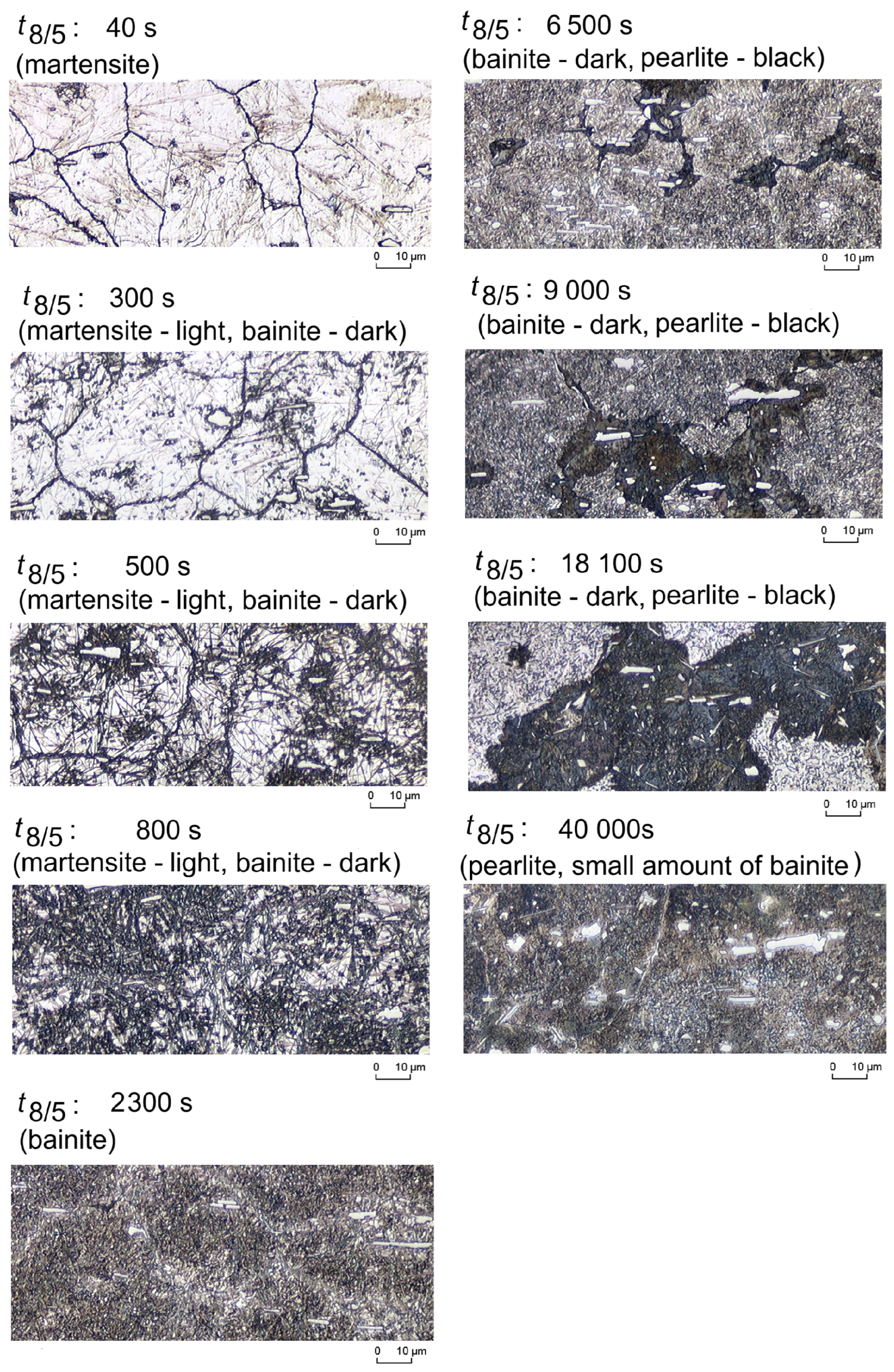
The samples obtained after the dilatometer experiments, during which the specified heat treatment is applied, are further examined using X-ray diffraction (XRD) and metallographic analysis. Microstructure analysis is conducted using light microscopy (LIMI). Light microscopic images of the dilatometer samples are then taken using an Olympus BX3M (Olympus Corporation, Tokyo, Japan) to determine the phase composition. Representative microstructures from LIMI are presented in Figure 1. Prior austenite grain size is about 55 µm. The width of the martensitic laths is in the order of 0.5 µm, and the lateral length is in the order of a few µm.
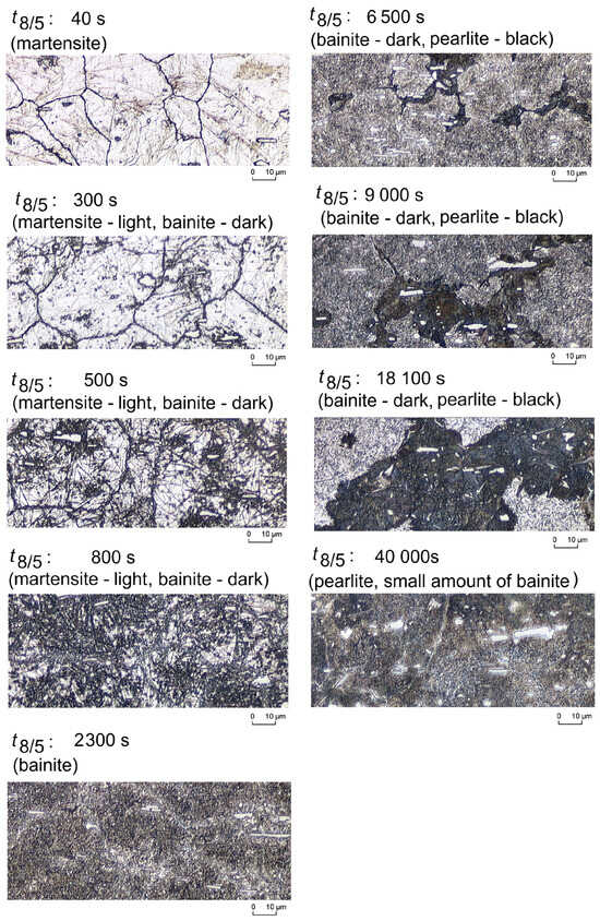
Figure 1.
Micrographs of martensite (cooling time: 40 s from 800 °C to 500 °C), martensite, small amount of bainite (cooling time: 300 s from 800 °C to 500 °C), martensite–bainite (cooling time: 500 s from 800 °C to 500 °C), martensite–bainite (cooling time: 800 s from 800 °C to 500 °C), bainite (cooling time: 2300 s from 800 °C to 500 °C), bainite–pearlite (cooling time: 6500 s from 800 °C to 500 °C), bainite–pearlite (cooling time: 9000 s from 800 °C to 500 °C), bainite–pearlite (cooling time: 18,100 s from 800 °C to 500 °C) and pearlite, small amount of bainite (cooling time: 40,000 from 800 °C to 500 °C).
Both characterization techniques (XRD and LIMI) enable the observation of various properties, including the crystal structure, crystal defects, phase composition, and microstructural features.
2.3. X-Ray Diffraction Measurements
The X-ray diffraction (XRD) experiments are conducted using a parallel beam geometry. The required mirror for parallel beam geometry suppresses K. As a result, the emission profile contains only K and K. A “D8 Advance diffractometer” (Bruker axs, Karlsruhe, Germany) equipped with a position-sensitive detector (PSD) is employed to realize a counting time for one diffractogram within 30 min.
The diffraction patterns are acquired with Cr-K radiation and not with Cu-K radiation. This choice is made to avoid strong fluorescence of ferrous samples, which occurs when exposed to Cu-K radiation. The high attenuation length of the Cr-K radiation compared with Cu-K radiation is another advantage of the Cr-K source.
The diffractograms are recorded over a range from (corresponding to a of 2.761 Å) to (corresponding to a of 1.199 Å) with a step size of . Further details can be found in [2,6].
2.4. Quantification of Phases
X-ray diffractograms are analyzed by the Rietveld method via a fundamental parameter model using Topas 3.0 of Bruker axs [7]. Measurements are conducted across the complete range using LaB6 (NIST 660a) as a reference material to determine and account for the instrument-caused peak broadening. Furthermore, the Double-Voigt model is used to differentiate between the size and strain components of defects found in the high-speed steel samples. A detailed description of this model can be found in [8]. An extensive Rietveld analysis of these samples can be found in [2]. The quantification of retained austenite and carbides (, ), and possibly trace amounts of , is also achieved using the Rietveld method. The mass fraction of austenite is presented as a function of the time in Table 2.
Table 2.
Retained austenite after cooling as a function of —cooling time for the steel HS1-5-1-8.
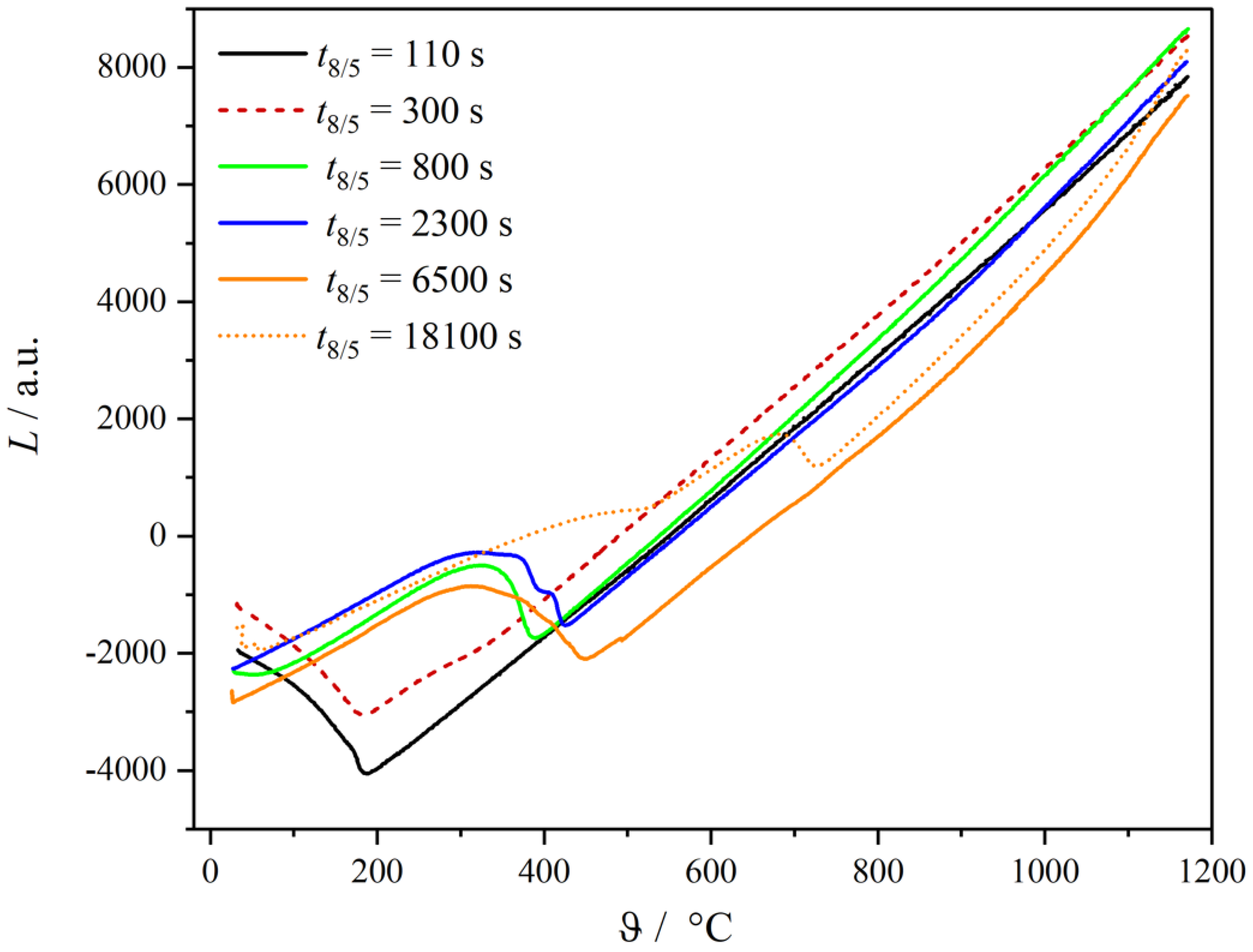
By means of the Rietveld method alone, it is difficult, if not impossible, to distinguish between martensite, bainite, and ferrite in pearlite due to their similar crystallographic structures and only slight variations in carbon content. Complementary methods to distinguish between these phases are the microstructural analysis by LIMI and dilatometric measurements. In the case of the LIMI method, differential etching using picric acid is applied. Different phases are etched to different degrees, and the resulting contrasts become visible during the LIMI investigation. Details about this method can be found in [9]. Dilatometry signals are evaluated on the basis of known thermal expansion coefficients of the face-centered austenite and of all body-centered phases, respectively. After austenitization, the slope of the temperature-dependent dilatometer curve is defined by the thermal expansion coefficient of austenite. Nearly identical coefficients of thermal expansion for the body-centered microstructures martensite, bainite, and ferrite can be assumed. However, martensite, bainite, and ferrite in pearlite are distinguishable due to different temperatures of transformation start and transformation end. This information is provided by the dilatometer experiment, which is evaluated in the form of a Time Temperature Transformation (TTT) diagram to be compared with TTT diagrams from literature. Verification of the presence of a phase is then conducted by LIMI analysis. Thereby, the temperature-dependent phase fractions of retained austenite, martensite, bainite, and ferrite within pearlite are determined. A detailed description and results of the complete phase quantification can be found in [2]. It is shown that the phase fraction determined by both micrographs and dilatometry gives the same results within the error margin. The sum of the volume fractions of martensite, bainite, and pearlite must equal unity. The volume fractions of martensite, bainite, and pearlite, as taken from [2], are presented in Table 3. For improved clarity, the results were obtained solely from etched micrographs. It is worth noting that the output of the micrographs corresponds to areas that align with the volume fractions (see Table 3). The dilatometry results, which present changes in length, are proportional to one-third of the volume changes. For fast cooling (black curve ), martensitic transformation occurs. Already for the second curve (), we see that there is a bainite transformation before the onset of the martensitic transformation. For , more bainite occurs before martensite. Austenite transforms to upper and lower bainite for (blue curve). An increasing amount of pearlite is detected for and 18,000 (orange and orange-dotted curve).
Table 3.
Relative volume fractions of martensite, bainite, and pearlite as a function of cooling time for HS1-5-1-8, including labeling.
The samples (1–10) listed in Table 3 have to be assigned to their classes. The samples with numbers (1–4) belong to class “martensite”, numbers (5–8) belong to class “bainite”, and samples (9–10) belong to “pearlite”. All samples are labeled by the following scheme called the one against all strategy [10]: The material is allocated to its class by the highest volume fraction of martensite or bainite or pearlite. The material gets “1” for this class and “−1” for the other two classes. For example, in sample 5, the volume fraction of bainite, which belongs to the bainite class due to the highest volume fraction of bainite, gets “−1” in the martensite column, “1” in the bainite column, and “−1” in the pearlite column. Each sample can only belong to one class.
The phase fractions determined by dilatometry, see Figure 2, are in good agreement with those obtained from the micrographs. The phase fractions in Table 3 are derived from the different colors of the etched phases. For labeling the data, the phase fractions obtained from LIMI are used.
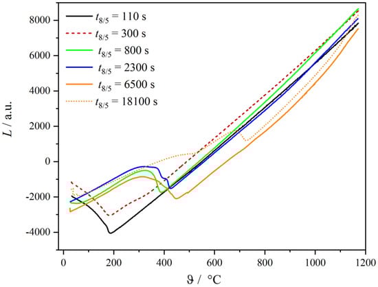
Figure 2.
Representative dilatometer curves depending on the cooling time.
The differentiation of the individual microstructures, martensite, bainite, and pearlite can be done by applying machine learning algorithms on the diffractograms of the differently heat-treated samples, as will be shown in this work. For the sake of simplicity, the focus will be solely on the phase fractions as a distinctive feature.
3. Machine Learning Algorithms
Three main types of machine learning algorithms are commonly used in practical applications: unsupervised learning, supervised learning, and reinforcement learning; details can be found, e.g., in the following textbooks [11,12,13]. In the following, the principles of unsupervised and supervised learning are briefly discussed as these techniques are used in this work:
- Unsupervised learning algorithms do not require labeled data for training. Instead, their objective is to discover patterns and structures within the data by clustering similar data points and identifying relationships between them; details can e.g., be found in [13]. The t-SNE algorithm used is described in Appendix A. Details of the agglomerative hierarchical clustering algorithm are presented in Appendix B.
- Supervised learning algorithms utilize labeled datasets, where each data point is assigned a label standing for a category. These labeled examples consist of input data along with their corresponding desired outputs. Through regression techniques, supervised learning algorithms analyze the labeled data to find the best-fitting model. Once the model is trained, it can be used to classify and assign new data to their categories [13]. Detailed information about the support vector machine can be found in Appendix C. The robustness of the support vector machine results is analyzed through cross-validation. The method is presented in Appendix D.
However, before the machine learning algorithms come into play, the experimental data have to be prepared and preprocessed as described in the next section.
3.1. Data Preparation and Preprocessing
Data preparation plays a crucial role in the analysis of diffractograms by ensuring the suitability of the data for clustering. To this aim, interfering properties such as variations in irradiated specimen surfaces, measurement time per step, and total X-ray tube intensity have to be taken into account.
Various methods are proposed in the literature for data preparation [14,15] with two main steps: normalization and mean subtraction. Some commonly used normalization methods are as follows:
- Min-max scaling [16]: This method rescales the data to a specific range, typically between 0 and 1, by subtracting the minimum value and dividing by the range.
- Z-score standardization [17]: This method transforms the data to have a mean of 0 and a standard deviation of 1. This is achieved by subtracting the mean from the original data. Division of the standard deviation of the subtracted data results in Z-score standardization.
- Power transformation [18]: This method adjusts the data distribution to conform more closely to a desired distribution or meet certain statistical assumptions.
- An alternative method for normalizing diffractograms involves dividing each diffractogram by its average value. In the case of a Principal Component Analysis (PCA) analysis, the mean value is subtracted from the normalized data. This newly introduced area-normalized method is related to the Rietveld method, where the quantitative results are normalized by the overall peak areas [19]. This area-normalized method is particularly recommended when the diffractograms undergo PCA for dimensionality reduction, as will be explained in the next subchapter. This reduces the impact of the mentioned problems, such as different irradiated sample areas, variations in the tube intensity, and different measuring times per step for different diffractograms.
The prepared data can then be used for dimensionality reduction, e.g., by PCA.
3.2. Dimensionality Reduction by PCA
Principal Component Analysis (PCA) is a widely used technique for dimensionality reduction in a dataset X.
In many cases, datasets, e.g., diffractograms, contain highly correlated features (e.g., two very similar austenite peaks). To address this issue and improve computational efficiency, dimensionality reduction methods are applied. Reducing the dimensionality not only enhances computational efficiency but also improves the predictive power of models by eliminating irrelevant features such as noise or background.
Several algorithms are available for computing principal components; frequently, Singular Value Decomposition (SVD) is used to execute PCA [20].
The output of PCA consists of two transformation matrices, namely the coefficient matrix W and the scores matrix U (details can be found in [21]):
- The orthogonal coefficient matrix W, also known as the loading matrix, represents the weights or coefficients that define the principal components in terms of the original variables.
- The orthogonal scores matrix U represents the original data expressed in the new principal component space (the rotated coordinate system).
The diffractogram is transformed by linearly mapping the data vector X via W into the transformation vector T containing the uncorrelated variables.
The transformed data T exhibit the following favorable characteristics:
- The variables become uncorrelated.
- The first few principal components, consisting of data in the rotated coordinate system (scores) and their weights (coefficients or loadings), capture the most crucial information, while the remaining components represent less significant variations or noise. The importance of individual components can be determined by the absolute values of their corresponding eigenvalues. Higher-order principal components can often be disregarded, leading to reduced dimensionality. The lost information corresponds to the sum of the ignored absolute eigenvalues in relation to the sum of all absolute eigenvalues.
- The original dataset can be reconstructed by multiplying T with the inverted matrix .
Only the first L entries of the principal components in the vector T are significant, resulting in the approximation:
where only the first L columns contain non-zero entries.
4. Results and Discussion
4.1. Preprocessing of Diffractogram Data
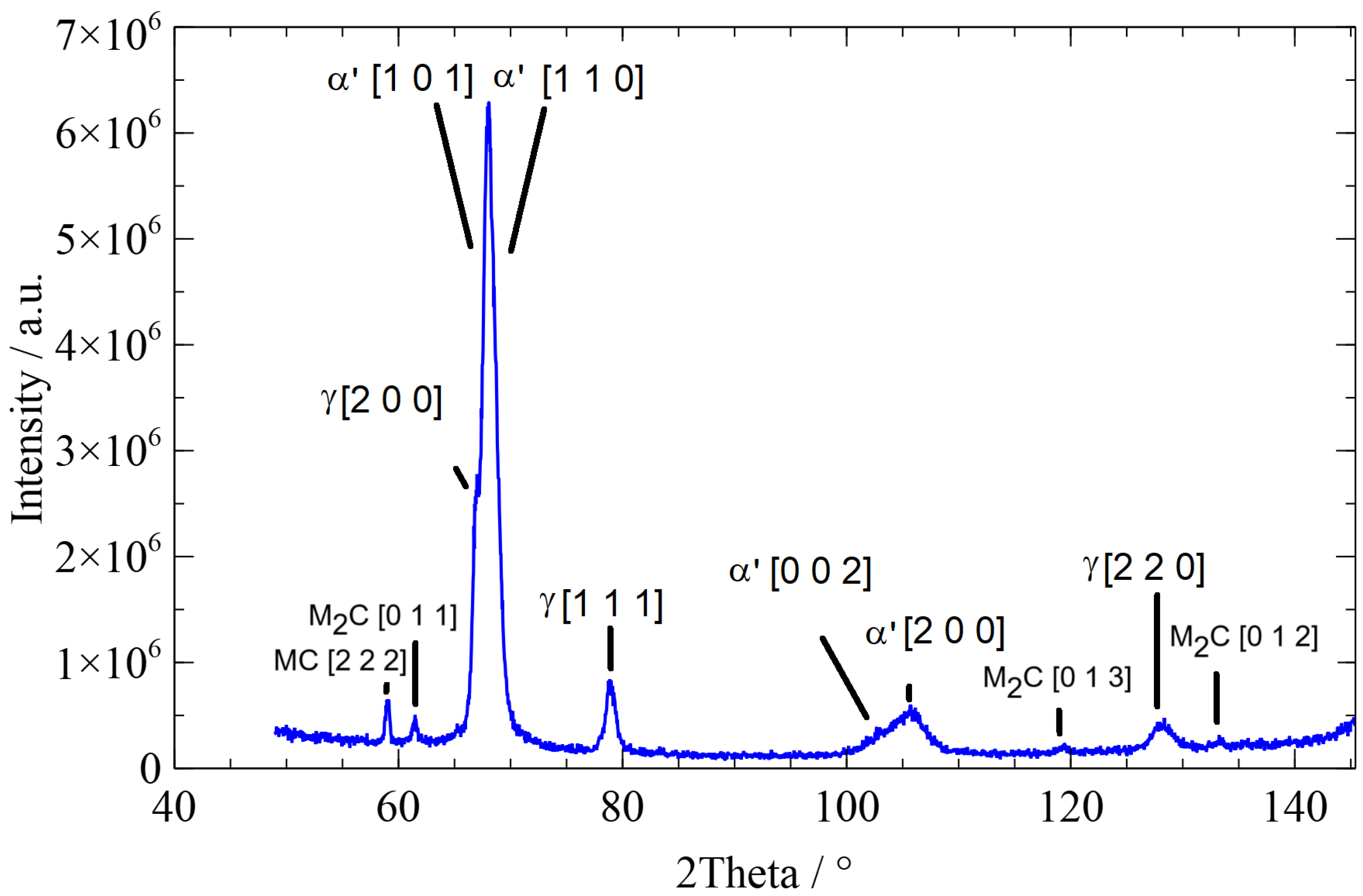
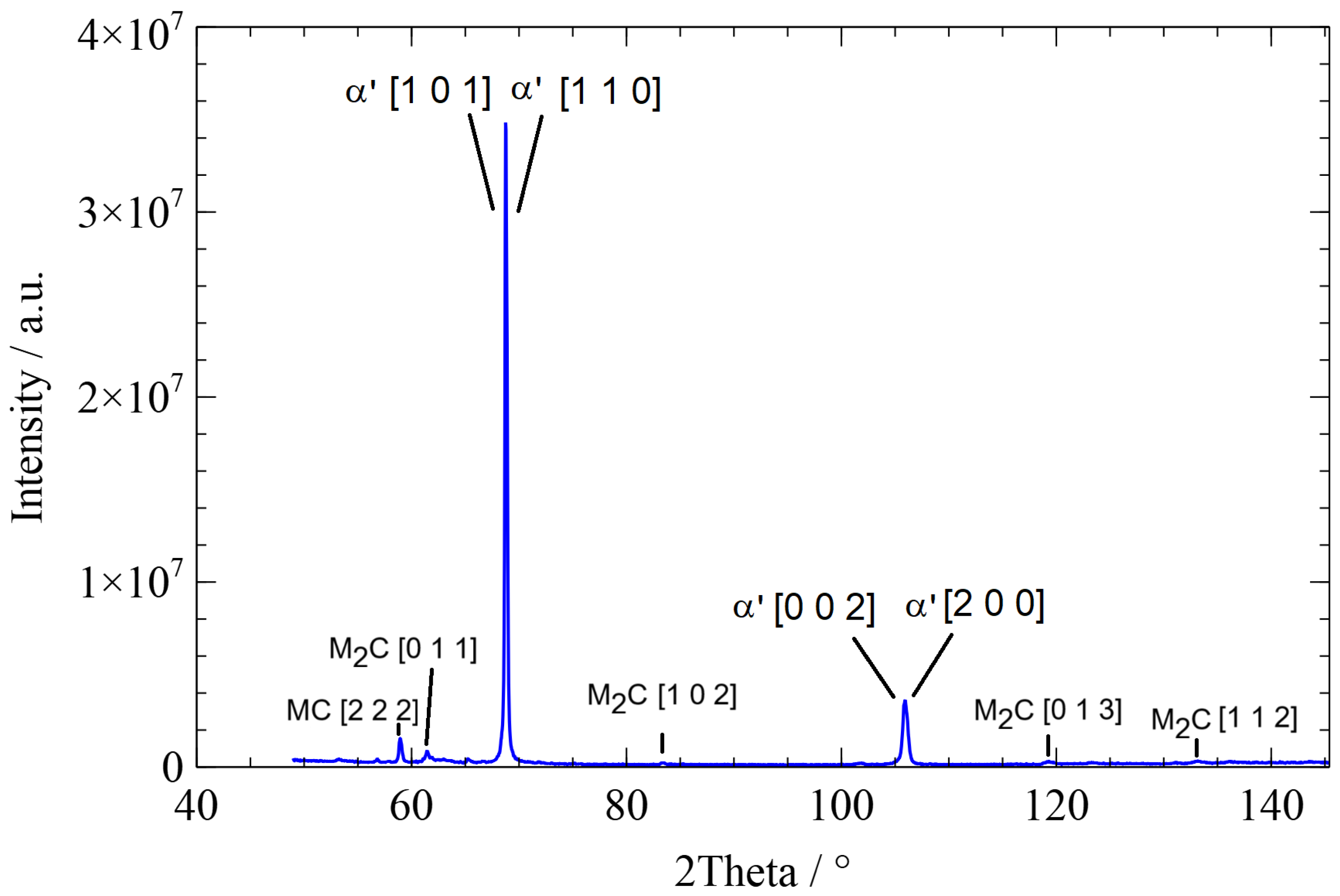
The following figures depict typical diffractograms of the three different microstructures, martensite, bainite, and pearlite. The diffractogram of a martensitic microstructure is presented in Figure 3, the diffractogram of a bainitic microstructure in Figure 4, and the diffractogram of a pearlitic microstructure in Figure 5. The different time characterizes the cooling rate, which is responsible for the evolution of the different microstructures.
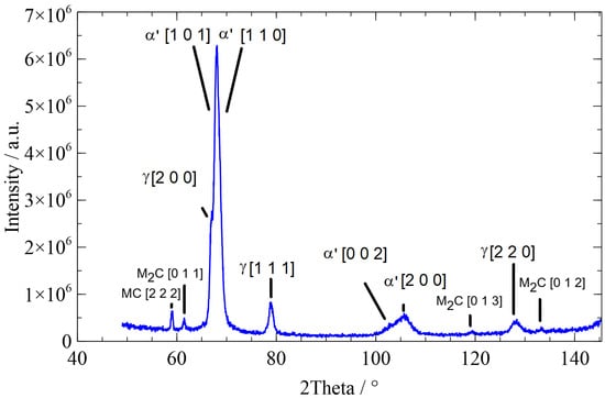
Figure 3.
Diffractogram of a martensitic microstructure with a time of 40 s: ’ …martensite, …austenite.
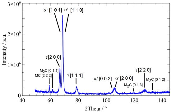
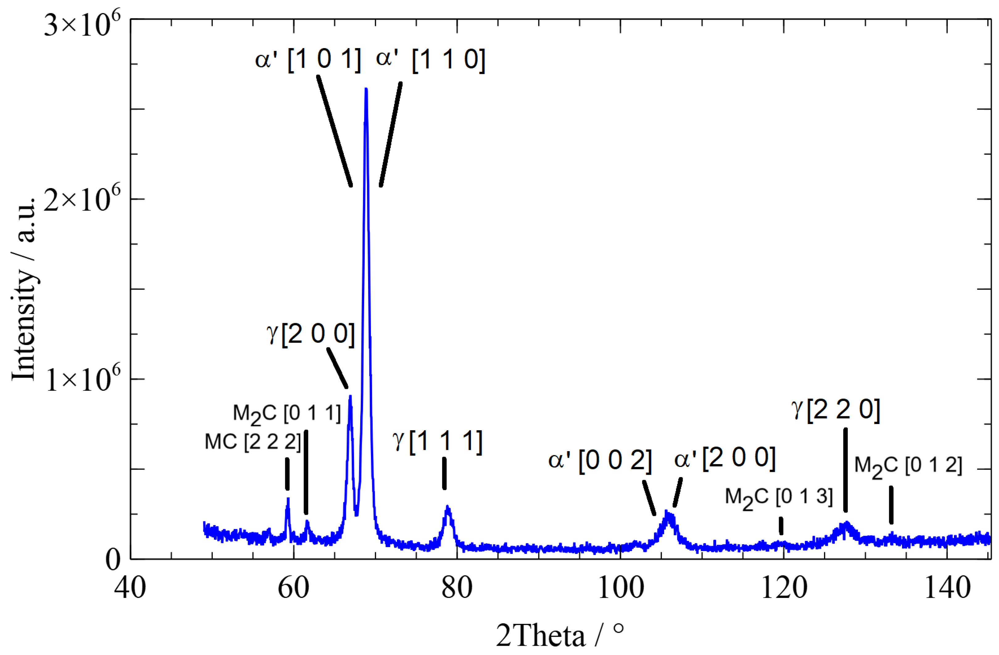
Figure 4.
Diffractogram of a bainitic microstructure with a time of 2300 s: ’ …bainite, …austenite.
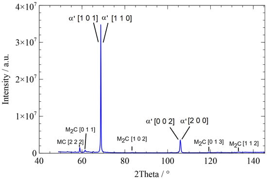
Figure 5.
Diffractogram of a pearlitic microstructure with a time of : ’ …ferrite in pearlite.
The widths of the martensite peaks are determined by the cooling rate-dependent amount of carbon dissolved in tetrahedral sites. In addition, the cooling rate-dependent dislocation density also influences the peak widths. The austenite peaks depend on the interstitially dissolved amount of carbon in austenite. Details can be found in [2,22,23].
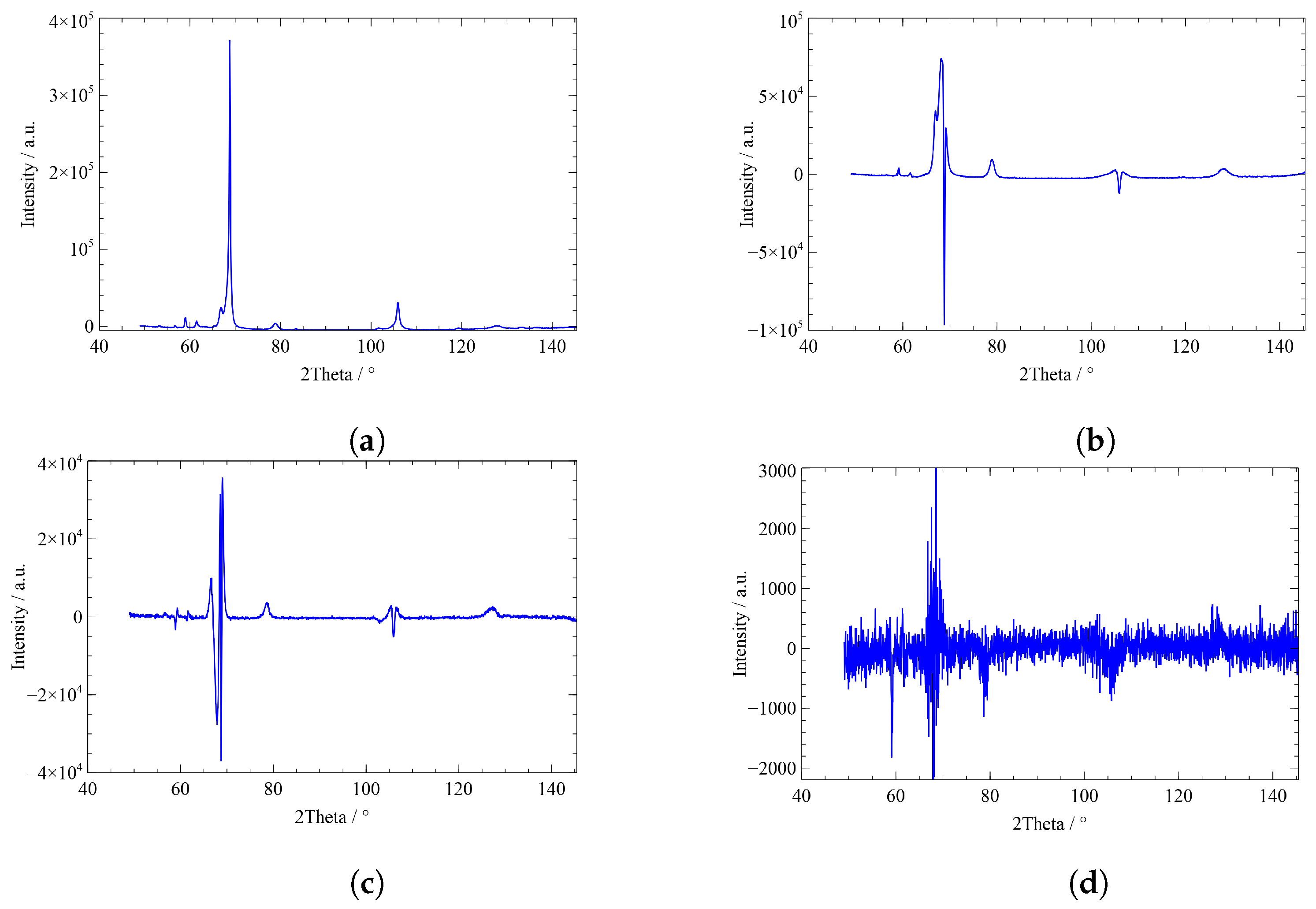
Diffractogram data are normalized by its average intensity value (area-weighted normalization), and the mean value is subtracted. Subsequently, PCA is performed on the normalized data. By means of principal component analysis, a system of transformed diffractograms (coefficients) is generated, from which the existing diffractograms can be reconstructed. The color-coded points indicate how much of each principal component (PCA1 or PCA2 or PCA3) is needed to represent the given diffractogram. The PCA scores (PCA1, PCA2, and PCA3) are prefactors that are multiplied with the coefficients. Figure 6 shows a section of this system. Principal component coefficients, or loadings, are the “weights” of the diffractograms. The first three coefficients (loadings) of PCA and the last coefficient (tenth) of PCA are presented in Figure 6. Whereas the first coefficient plotted versus contains a high amount of information, and the second and third coefficients are also required, the tenth coefficient contains only random noise.
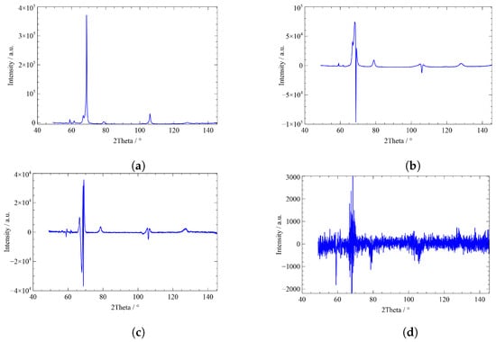
Figure 6.
First three coefficients and last coefficient of the PCA analysis. (a) First coefficient, (b) second coefficient, (c) third coefficient, (d) last (tenth) coefficient.
The scores of the principal component coefficients are listed in Table 4.
Table 4.
First three of the ten scores of the principal component coefficients (PCA1, PCA2, and PCA3) for the 10 diffractograms with increasing time.
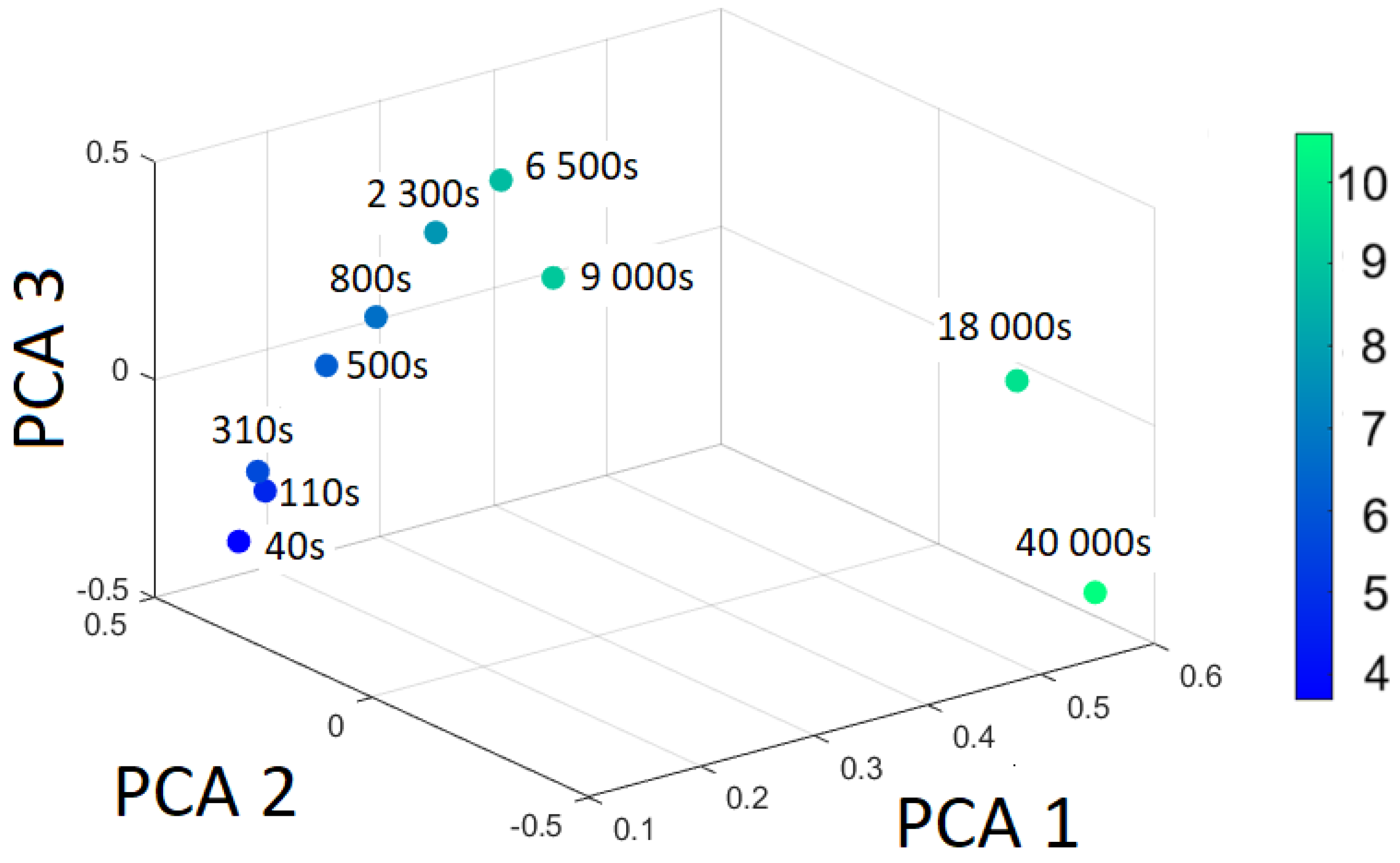
The principal component scores from Table 4 are illustrated in Figure 7. The color-coded points in Figure 7 are scaled by with the color bar shown on the right side.
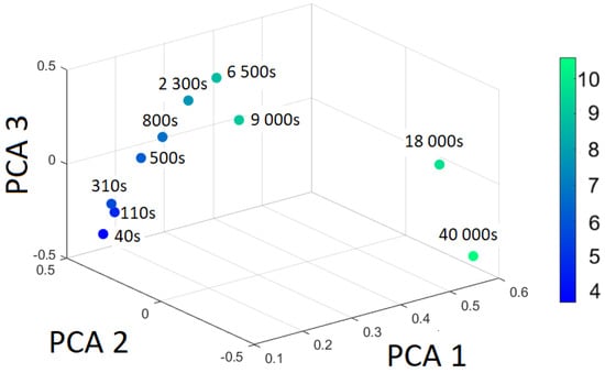
Figure 7.
The first three PCA scores (transformed data) for the different cooling temperatures.
From the eigenvalues follows that the first component accounts for 80.0% of the variance, the second component explains 16.8%, and the third component captures 2.3%.
In other words, the 10-dimensional problem (10 diffractograms are used) can be reduced to 2 or 3. Principal components higher than 3 do not contain useful information. In the next section, the preprocessed data are analyzed by unsupervised (e.g., hierarchical clustering and t-SNE) and supervised machine (e.g., support vector machine) learning algorithms.
4.2. Machine Learning Algorithm Applied to XRD Data
4.2.1. Agglomerative Hierarchical Clustering of XRD Data
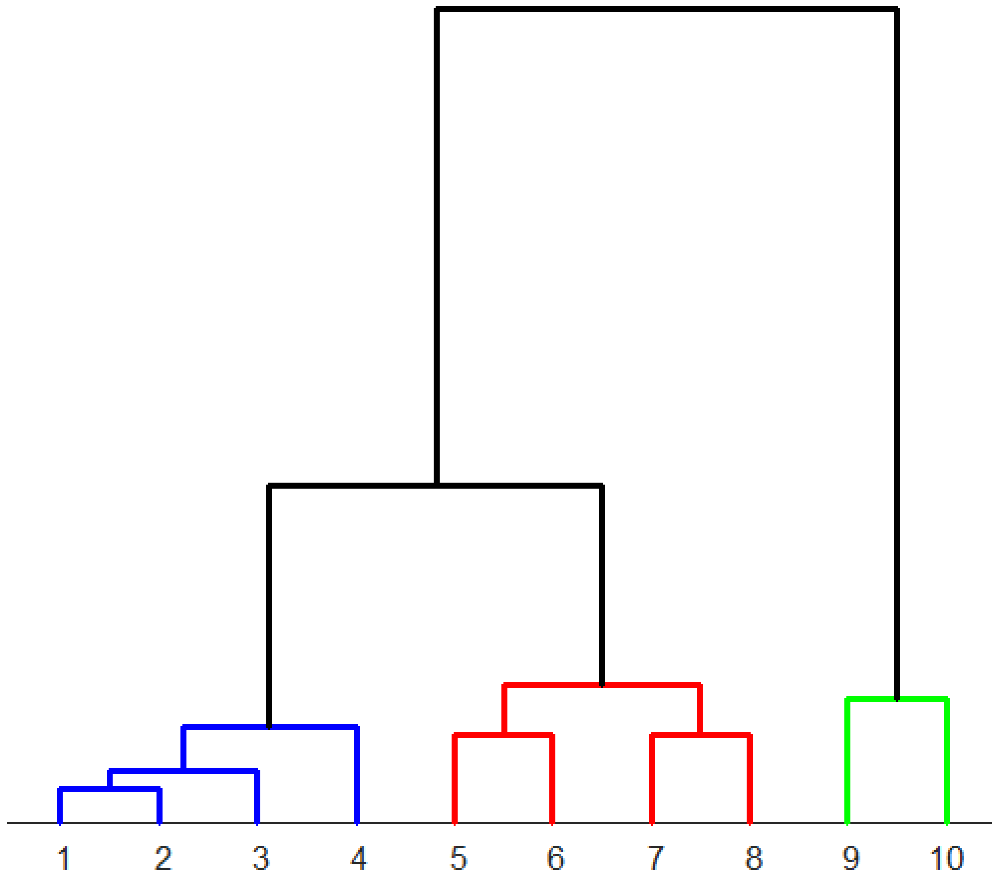
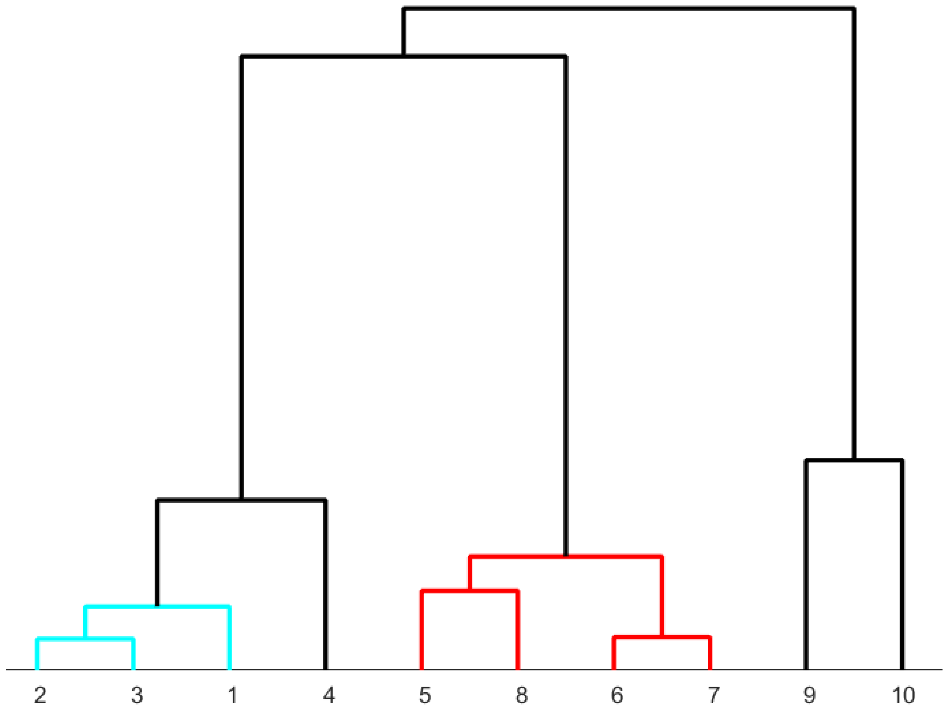
The analysis of the area-normalized diffractograms by hierarchical clustering results in a dendrogram presented in Figure 8. The distance measure is based on the Euclidean norm. Thereby, the dissimilarity of the diffractograms is computed. As a linkage method, the “ward” method [24] is used for choosing the pair of clusters to merge at each step. The linkage is calculated by the recursive Lance–Williams algorithms [25].

Figure 8.
Dendrogram to classify ten differently heat-treated high-speed steels determined from the area-normalized diffractograms. The microstructures assigned to the numbers can be found in Table 3. Colors: blue: predominantly martensite, red: predominantly bainite, green: predominantly pearlite.
According to the dendrogram in Figure 8, the two samples (samples 1 and 2) with fully martensitic composition exhibit the highest similarity. Samples 3 and 4, which are also predominantly martensitic, cluster closely together. The predominantly bainitic samples (samples 5, 6, 7, and 8) are clustered together. The predominantly pearlitic samples (9 and 10) form a distinct class. In summary, the results obtained from the area-normalized diffractograms show a pattern that clustered together similar microstructures.
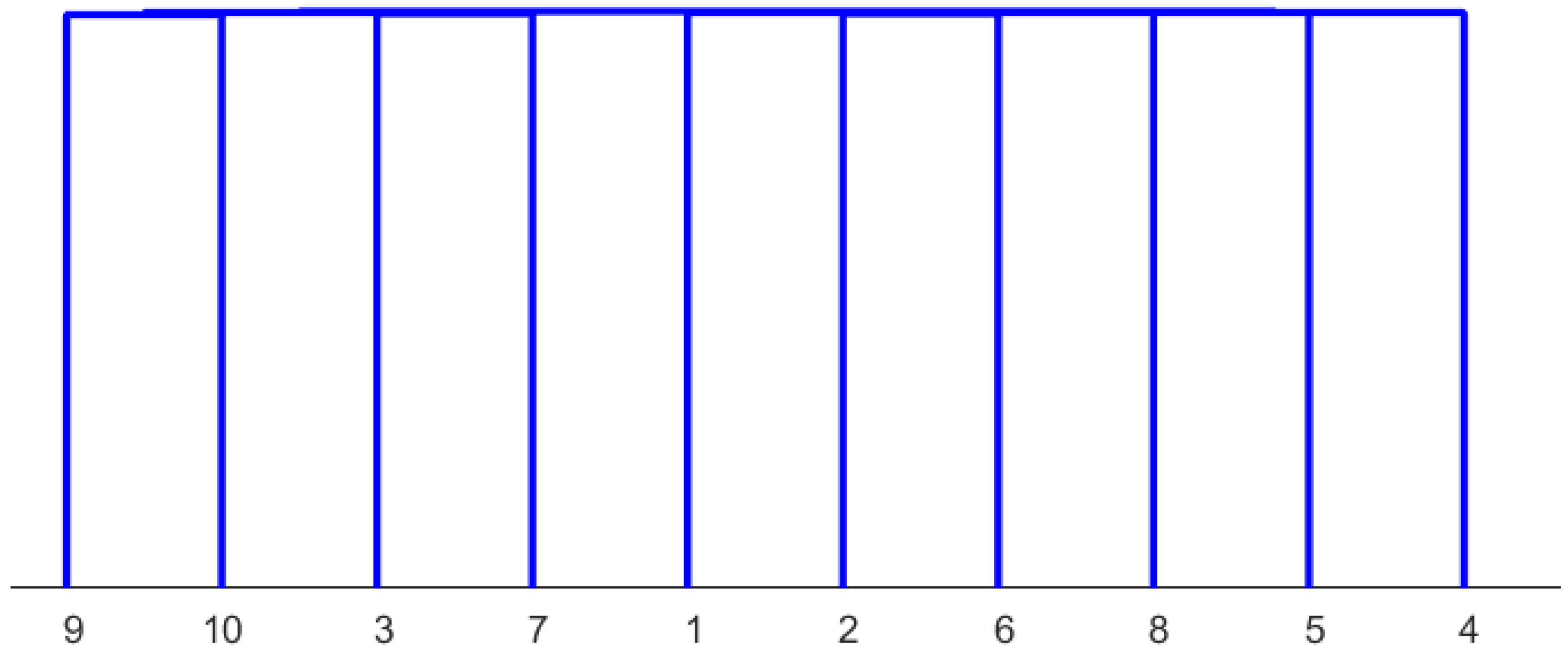
Other normalization methods do not yield satisfactory results. An example using Z-score normalization is shown in Figure 9. It is, e.g., evident that samples 2 and 3 have a more different microstructure than samples 2 and 1, but 2 and 3 are clustered together. Further, samples 5 and 7 as well as 6 and 8 are clustered, where a clustering of 5 with 6 and 7 with 8 would better represent reality.
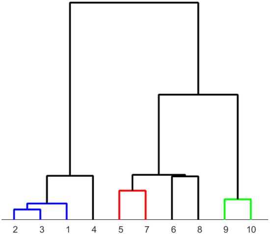
Figure 9.
Dendrogram determined from Z-score normalized diffractogram using the Euclidean norm and “ward” as the linkage method. The microstructures assigned to the numbers can be found in Table 3.
Thus, area normalization is superior to other normalization methods (e.g., Z-score normalization as shown here). The reasons are as follows: Area normalization works since the relative amounts of the phase fractions are considered by this normalization technique. In other words, the areas of the peaks—which are proportional to the phase fractions—are characteristic features of the diffractograms and are not corrupted by this normalization technique. Differences in the diffractograms, including peak widths and peak heights, are analyzed by the Euclidean norm.
In comparing the results of hierarchical clustering using area-normalized data and PCA-transformed data, they are presented in Figure 10. The sorting appears completely random when the complete transformed data are used to construct the dendrogram. In this figure, the algorithm’s challenges with noise become apparent.
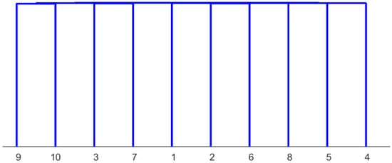
Figure 10.
Dendrogram constructed from all PCA components. These components are computed from the area-normalized diffractogram using the Euclidean norm and the “ward” linkage method. The microstructures assigned to the numbers can be found in Table 3.
An illustrative example involving three factor loadings is presented in Figure 11. As mentioned earlier, the third PCA component contains minimal additional information, representing only 2.3% of the variance. It’s worth noting that this component carries the same weight as the first component, which accounts for 80.0% of the variance. However, the third component also exhibits a significant level of noise, as evident in Figure 6c.

Figure 11.
Dendrogram generated from the first three PCA components. These components are computed from the area-normalized diffractogram using the Euclidean norm and the “ward” linkage method. The microstructures assigned to the numbers can be found in Table 3.
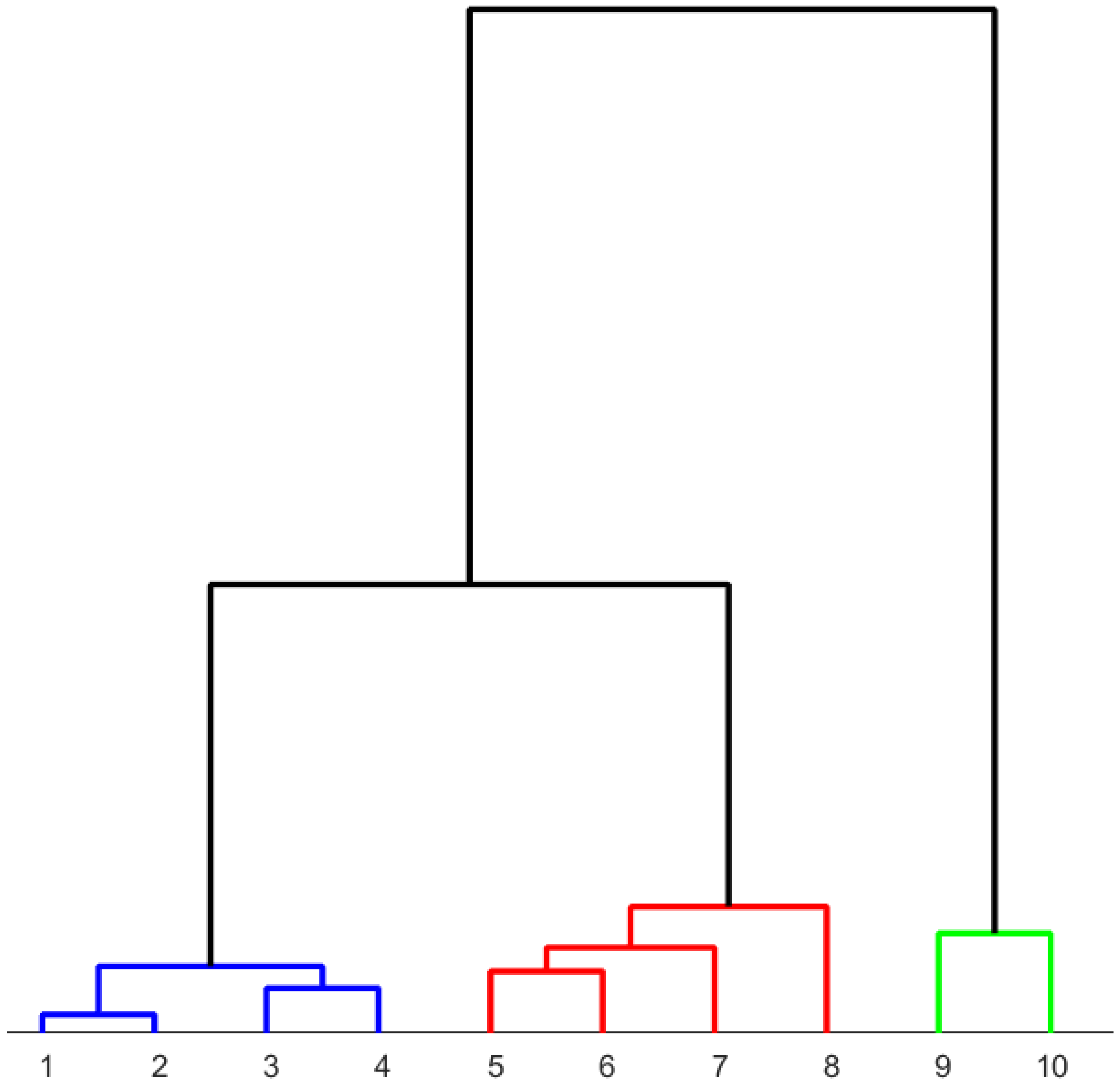
However, when hierarchical clustering is performed using only the first two factor loadings, the resulting dendrogram (Figure 12) is similar to the dendrogram obtained from the normalized XRD data in Figure 8.
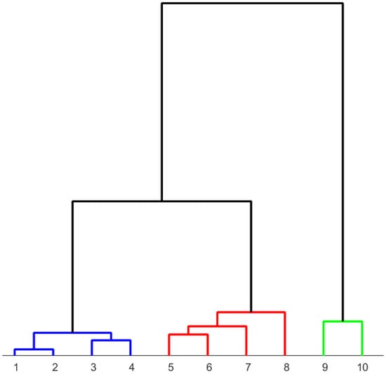
Figure 12.
Dendrogram constructed from the 1st and 2nd PCA components. These components are computed from the area-normalized diffractogram using the Euclidean norm and the “ward” linkage method. The microstructures assigned to the numbers can be found in Table 3. Colors: blue: predominantly martensite, red: predominantly bainite, green: predominantly pearlite.
Increasing the dimensionality in this manner negatively impacts the performance of the hierarchical clustering algorithm. Therefore, it is advisable to perform hierarchical clustering on the normalized diffractograms directly.
In summary, hierarchical clustering yields good results for area-weighted diffractograms, but analyzing PCA data depends significantly on the number of factor loadings considered. As it is difficult to predict how many factor loadings need to be taken into account for a good result, this method is not recommended.
4.2.2. t-SNE Analysis of XRD Data
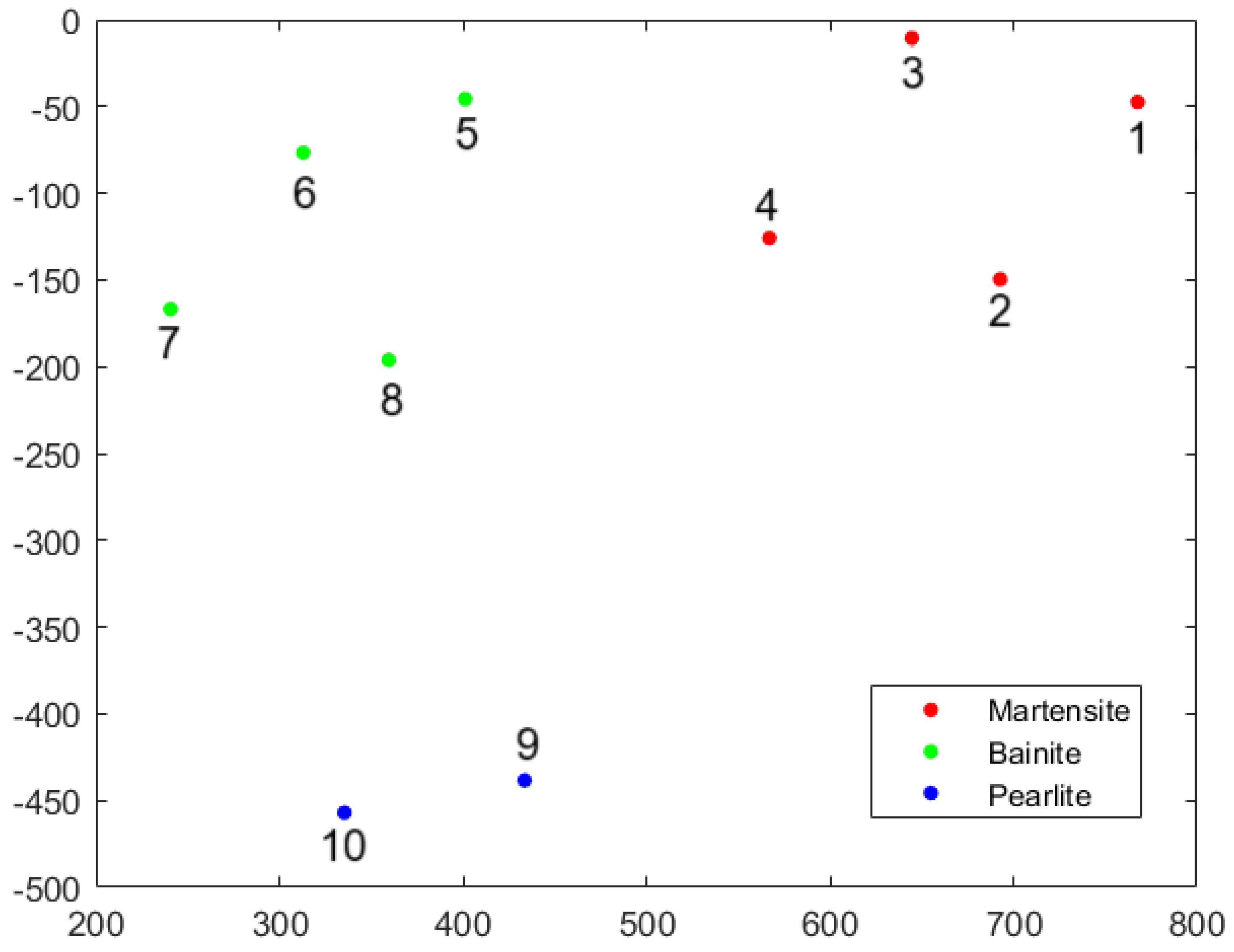
The area-normalized diffractograms are used to visualize similarity data using the t-SNE method. This approach retains the local structure of the data while also revealing significant global structures such as clusters [5].
Any new dataset should be analyzed with corresponding labeled measurements using t-SNE. Depending on where the new dataset is located afterwards, the existing microstructure can be determined from the diffractogram alone. As demonstrated in Figure 13, martensite, bainite, and pearlite are reasonably separated into different clusters. A summary of the labels can also be found in Table 3.
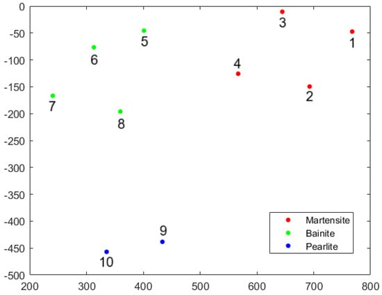
Figure 13.
Visualization of t-SNE analysis from area-normalized diffractograms.
A certain drawback of this method is that with every analysis, the results are slightly different (e.g., the mapping is rotated). However, this will not compromise the principal outcome.
4.2.3. Support Vector Machines to Separate Phases by Hyperplanes
In this subchapter, the application of support vector machines (SVM) to the task of separating phases through hyperplane classification is explored. The hinge loss function serves as the chosen objective function in this maximum-margin SVM. Raw data from the measurements have to be preprocessed, including a PCA transformation as a prerequisite for the SVM model training. The one-against-all strategy enables the classification of samples into their respective classes based on the decision boundaries determined by the SVM model. Here three distinct microstructural conditions (“martensite”, ”bainite”, and “pearlite”) are separated by means of support vector machines (SVM). The classifications (labels) are taken from Table 4.
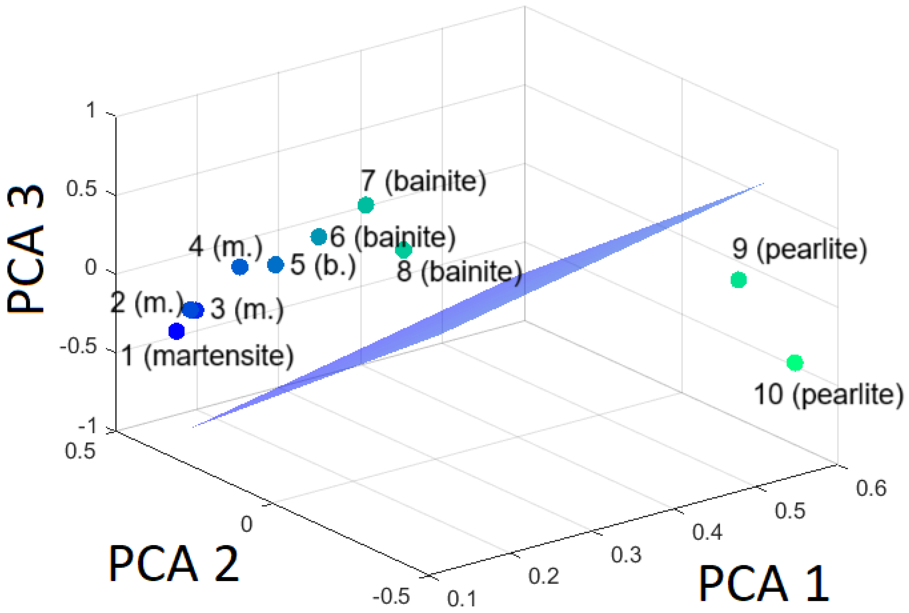
Figure 14, Figure 15 and Figure 16 are presented to visualize the hyperplanes in relation to the three classes, demonstrating the selectivity of the SVM model.
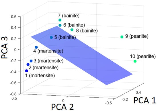
Figure 14.
Hyperplane separating martensite from the rest (bainite and pearlite) based on the first three principal components.
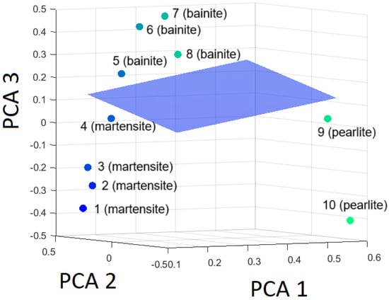
Figure 15.
Hyperplane separating bainite from the rest (martensite and pearlite) based on the first three principal components.
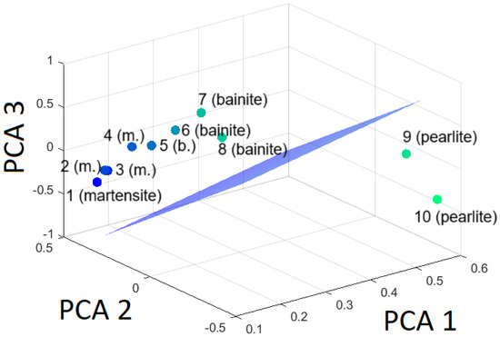
Figure 16.
Hyperplane separating pearlite from the rest (martensite and bainite) based on the first three principal components.
It has been established that separation is achievable without any difficulties.
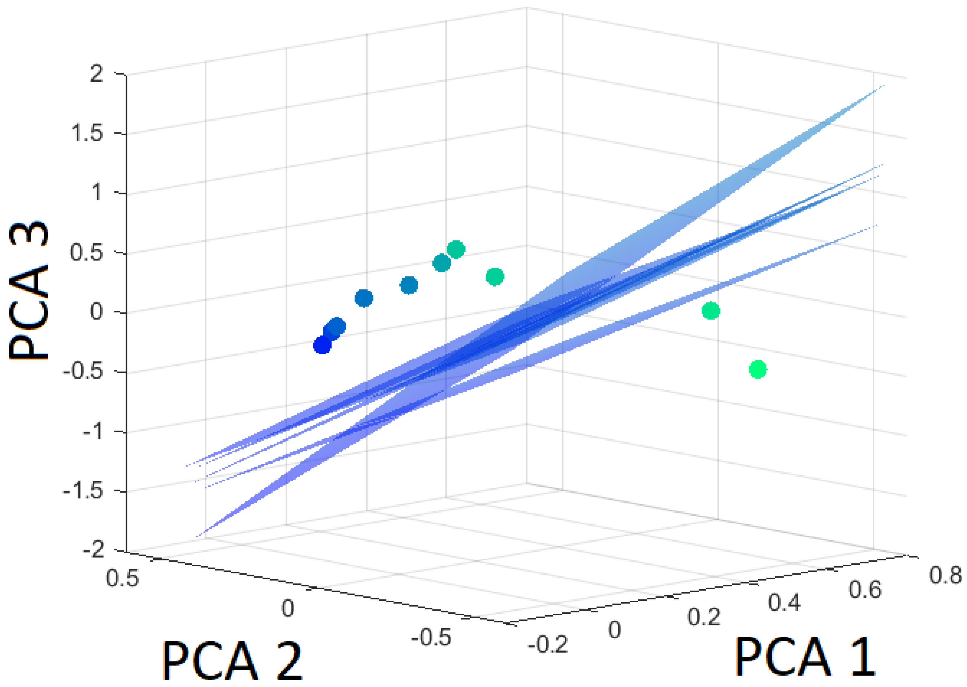
The robustness of the SVM algorithm is determined by the Leave-One-Out Cross-Validation (LOOCV). First, the distances to the hyperplane are computed for all ten datasets. Then, the hyperplane is calculated with one dataset left out. The distance of this altered hyperplane to the left-out dataset is determined. Thereby, a measure for the uncertainty of the hyperplane is computed. The individual altered hyperplanes are presented in Figure 17, Figure 18 and Figure 19.
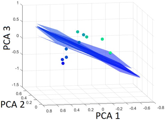
Figure 17.
Hyperplanes separating martensite from the rest (bainite and pearlite) using Leave-One-Out based on the first three principal components.
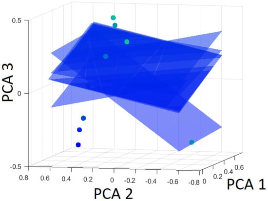
Figure 18.
Hyperplanes separating bainite from the rest (martensite and pearlite) using Leave-One-Out based on the first three principal components.

Figure 19.
Hyperplanes separating pearlite from the rest (martensite and bainite) using Leave-One-Out based on the first three principal components.
When the distance of the dataset to the hyperplane is given with a positive sign, then the dataset belongs to the class that is separated from the other classes by the hyperplane. On the contrary, a negative value indicates it belongs to the rest. The distances to the altered hyperplanes with martensite separated from the rest are presented in Table 5. As evident from Table 5 and Figure 17, the distance of the omitted data point from the hyperplane barely changes, indicating strong robustness.
Table 5.
Calculation distance to hyperplane of martensite to rest by Leave-One-Out Cross-Validation (LOOCV) compared with all data points as a function of cooling time for HS1-5-1-8.
In the following, the hyperplane that separates bainite from the martensite and pearlite is investigated by the LOOCV technique. The altered hyperplanes are presented in Figure 18. Not all datasets are correctly classified after using the LOOCV test. Datasets 4 and 9 are misclassified, as can be seen in Table 6. As evident from Table 6 and Figure 18, the distance of the omitted data point from the hyperplane noticeably changes, indicating weak robustness. The hyperplane is nearly parallel to PCA 3. That means that changes in this hyperplane are changes in PCA 3. As mentioned earlier, PCA 3 only accounts for 2.3% of the variance.
Table 6.
Calculation distance to hyperplane of bainite to rest by Leave-One-Out Cross-Validation (LOOCV) compared with all data points as a function of cooling time for HS1-5-1-8.
The variation of the hyperplane that separates pearlite from the other classes is calculated according to the LOOCV test. The different hyperplanes due to leaving out a distinct dataset are presented in Figure 19.
All datasets are classified correctly for all altered hyperplanes in case pearlite is to be separated from all other classes. The distances of the datasets to the original and to the altered hyperplanes have the same sign for all cases (Table 7). Figure 19 clearly shows that the distance of the omitted dataset from the hyperplane exhibits minimal change, underscoring its strong robustness.
Table 7.
Calculation distance to hyperplane of pearlite to rest by Leave-One-Out Cross-Validation (LOOCV) compared with all data points as a function of cooling time for HS1-5-1-8.
It can be stated that the hyperplanes separating martensite from the rest (bainite and pearlite) and pearlite from the rest (martensite and bainite) have been found to be highly robust during cross-validation. The hyperplane that separates bainite from the rest (martensite and pearlite) appears to be unstable and heavily influenced by individual data points.
5. Conclusions and Outlook
In this study, we conducted a comprehensive analysis of microstructure evolution in high-speed steels by employing materials characterization techniques and machine learning algorithms. Data normalization was crucial to ensure the appropriate application of the machine learning algorithms.
Standard normalization methods such as “Z-Score” or “Min-max” do not provide satisfactory results for the diffraction data analyzed in this work. However, “area normalization”, which is related to data preparation in the Rietveld method, works well.
The main results of this work are summarized as follows:
- After “area-normalization” of the diffraction data, the different material classes “martensite”, “bainite”, and “pearlite” are successfully grouped by agglomerative hierarchical clustering as well as by the t-SNE method.
- PCA is an effective method to eliminate irrelevant information and serves as a prerequisite for the setup of SVMs. Problems occurred using PCA-transformed data in hierarchical clustering because the algorithm is sensitive to noise.
- By means of support vector machines (SVM), different microstructures in steels can be distinguished on the basis of diffractograms only. To maximize SVM effectiveness, the data must be transformed using principal component analysis (PCA).
- LOOCV serves as an appropriate method for assessing the accuracy of the hyperplanes generated by SVM.
The methodology presented in this work appears particularly well suited for in situ observations, where a large number of XRD diffractograms are available. In such cases, the approach can efficiently cluster similar diffractograms.
It is expected that machine learning algorithms investigated in this work on a small scale are applied to monitor the evolution of the microstructure during materials processing in the future.
Author Contributions
Conceptualization, M.W. and E.G.; methodology, M.W. and E.G.; software, M.W.; validation, M.W. and E.G.; formal analysis, M.W. and E.G.; investigation, M.W. and E.G.; resources, M.W. and E.G.; data curation, M.W. and E.G.; writing—original draft preparation, M.W. and E.G.; writing—review and editing, M.W. and E.G.; visualization, M.W. and E.G.; supervision, M.W. and E.G.; project administration, M.W. and E.G. All authors have read and agreed to the published version of the manuscript.
Funding
This research received no external funding.
Data Availability Statement
The measurement data are available on request from the authors.
Conflicts of Interest
Manfred Wiessner was employed by DUAL Analytics. The remaining authors declare that the research was conducted in the absence of any commercial or financial relationships that could be construed as a potential conflict of interest.
Abbreviations
The following abbreviations are used in this manuscript:
| LIMI | Light Microscopy |
| LOOCV | Leave-One-Out Cross-Validation |
| PCA | Principal Component Analysis |
| SVM | Support Vector Machine |
| t-SNE | t-distributed stochastic neighbor embedding |
| TTT | Time-Temperature-Transformation |
| XRD | X-Ray Diffraction |
Appendix A. Dimensionality Reduction with t-Distributed Stochastic Neighbor Embedding (t-SNE)
Stochastic neighbor embedding, originally developed by Geoffrey Hinton and Sam Roweis, is an algorithm to visualize high-dimensional data [4]. Following [4], high-dimensional objects, which are, e.g., the vectors containing the data points of the diffractograms, are placed in a low-dimensional space. This is performed in a way that preserves neighbor identities. Laurens van der Maaten and Geoffrey Hinton proposed the t-distributed variant, as the visualizations produced by t-SNE are significantly better [5] than the original stochastic neighbor embedding algorithm.
However, one limitation of this method is that it does not allow for the straightforward addition of new elements to the existing embedding. Instead, to compare a new element with the other elements, a complete re-evaluation must be performed.
Appendix B. Unsupervised Learning Using Hierarchical Clustering
Hierarchical clustering is a fundamental technique in unsupervised learning that aims to group similar data points together based on their intrinsic characteristics or patterns. The primary goal of clustering is to uncover hidden structures or relationships within the data without relying on any prior knowledge of class labels or target variables. Renowned textbooks by Raschka and Mirjalili [11], Frochte [12], and Brunton et al. [13] provide comprehensive insights into this topic, and numerous clustering algorithms are available. Agglomerative hierarchical clustering was demonstrated for XRD data in the pioneering work by Barr et al. [26]. The clustering process involves several steps, including feature extraction and preprocessing, selecting a distance metric to measure similarity, and performing the actual clustering. Various metrics are presented and discussed in [27]. It is a goal of our work to apply the most suitable metric to the X-ray diffractograms and determine its impact on the results. It is worth noting that the choice of metrics strongly depends on the problem in general and the measurement data in particular. In this study, we specifically focus on the application of agglomerative hierarchical clustering using Euclidean distance. The agglomerative hierarchical clustering algorithm can be described as follows:
- First, the similarity matrix is computed, which quantifies the similarity between all pairs of data points. This is achieved using a distance metric, such as the Euclidean distance, which measures the dissimilarity between two data points based on their feature values. A known problem of the Euclidean metric is its sensitivity to outliers due to the quadratic norm.
- Initially, singleton clusters are created, i.e., treating each data point as a separate cluster.
- In the next step, a similarity matrix is computed between all singleton clusters using the Euclidean metric.
- The different clusters are grouped in a cluster tree by using an iterative linkage process. The linkage function accesses the similarity matrix to determine the ordering in the hierarchical cluster tree. The similarity between clusters can be defined in different ways, such as single linkage. Alternative linkage methods include complete linkage, average linkage, and centroid linkage, each offering different approaches to assess the similarity between clusters. Detailed information on these linkage methods can be found in [11,12,13].
It is an advantage of hierarchical clustering compared with other clustering methods that hierarchical relationships within the data are discovered. Furthermore, the result of the hierarchical clustering can be presented in a dendrogram, which provides a clear visualization of the relationships between data points.
While hierarchical clustering offers several advantages, this technique also comes along with drawbacks. Firstly, it exhibits computational complexity, particularly when dealing with large datasets. In such cases, alternative clustering algorithms like k-means or Density-Based Spatial Clustering of Applications with Noise (DBSCAN) [28], specifically designed for handling larger datasets and providing improved scalability, may be more suitable choices. Another limitation of hierarchical clustering is its sensitivity to noise and outliers. The presence of noisy data points and outliers can disrupt the clustering structure and potentially lead to inaccurate results. To address this issue, preprocessing techniques such as outlier detection and data transformation have to be applied to the raw data. These techniques may mitigate the impact of outliers on the clustering process, meaning that the overall robustness of the results is improved. An alternative approach involves the use of distance metrics that are robust to outliers, such as the well-known Huber loss function [29].
In the following paragraph, supervised machine learning tools are introduced, since they will also be applied to analyze and categorize the diffractograms.
Appendix C. Supervised Learning with a Support Vector Machine (SVM)
Data need to be prepared and transformed by techniques like PCA for dimensionality reduction before the SVM algorithm can be used properly. This transformation by PCA not only improves computational efficiency but also helps to mitigate the risk of overfitting.
Subsequently, the SVM is applied to this transformed dataset. In addition, an appropriate kernel function is used to transform the data for SVM.
No existing kernel function seems a priori suitable for XRD data. Consequently, the decision was made not to further pursue this approach. After applying PCA to transform the XRD data, a classical Euclidean distance metric is used to separate the different diffractograms.
The SVM algorithm’s core task is to determine the optimal hyperplane that effectively separates the data into desired classes. This is achieved by solving an optimization problem that maximizes the margin between classes while minimizing misclassifications. The SVM’s objective function is designed to balance these competing goals. Different regression algorithms are applied to machine learning problems. Details can be found in [11,12,13].
Three types of algorithms are presented, which all maximize the margin between the classes but handle misclassifications and error tolerance differently. It depends on the problem set which regression method should be used. In the following, the three algorithms (hard-margin SVM, soft-margin SVM, and maximum-margin SVM using the “Hinge Loss Function”) are shortly introduced:
- Hard-margin SVM [30]: When two classes of examples can be separated by a hyperplane (i.e., they are linearly separable), there are typically infinitely many hyperplanes that can separate the two classes. The hard-margin SVM selects the hyperplane with the maximum margin among all possible separating hyperplanes. The formulae and definitions used here follow the textbook [11], and slight variations in definitions may appear in different literature. In this reference, it is shown that the margin can be expressed aswhere represents the normal vector of the hyperplane, and denotes the Euclidean norm of this vector. It does not have unit length in this formulation, according to [11], and is referred to as the “weight vector”. This is equivalent to solving the following minimization problem by optimization of and the bias term b:At the same time, all data points must satisfy the condition for correct classification:where is the x-coordinate of the position vector of data point i. corresponds to the class labels of the training data; in the direction of in the opposite direction to , b stands for the bias term, and signifies the Euclidean norm (length) of the weight vector.The objective of this optimization problem is to minimize the Euclidean norm of the weight vector , which maximizes the margin between the hyperplane and the support vectors. The inequality is the constraint in order to ensure that the training samples are correctly classified. Thus, each training sample must satisfy the condition that the product of its class label and its signed distance from the hyperplane is greater than or equal to 1. Since it requires all data points to be perfectly separable without violating this margin, it performs poorly during the following instances:
- (a)
- Data are not perfectly separable: In real-world datasets, perfect linear separability is rare, especially in the presence of overlapping classes or mislabeled data. Hard-margin SVM fails in such scenarios as it cannot accommodate errors.
- (b)
- Outliers significantly affect the decision boundary: Even a single outlier can drastically influence the hyperplane, leading to a poorly generalized model. Hard-margin SVM does not tolerate violations of the margin, which makes it unsuitable for noisy datasets.
Therefore, in the case of not perfectly separable data, a better approach is the soft-margin SVM. - Soft-margin SVM [31]:The soft-margin SVM allows for a certain degree of misclassification. In this scenario, additional slack variables are introduced into the optimization problem, and a penalty parameter C controls the trade-off between maximizing the margin and tolerating misclassifications.The mathematical formulation for the soft-margin SVM, as indicated by Raschka (2019) [11] and Frochte (2020) [12], is as follows:subject toHere, represents the slack variables accommodating misclassifications, while C serves as the penalty parameter that balances achieving a wider margin with permitting misclassifications.In practice, hard-margin and soft-margin SVMs are commonly employed choices. However, the central finding of the analysis by Rosasco (2004) [32] reveals that, particularly for classification purposes, the hinge loss emerges as the preferred loss function. This is attributed to the hinge loss function’s ability to yield better convergence compared with the conventional squared loss mentioned in hard-margin and soft-margin SVM.
- Maximum-margin SVM using the hinge loss function [32]:In supervised learning, the hinge loss function is a frequently chosen objective function. The hinge loss function, denoted as , for the data point i is defined by Equation (A7):In the hinge loss function, represents the labeled outcome, taking +1 if it belongs to the class and −1 if it does not. Further, the output of the classifier , computed as:The hinge loss function measures the difference between the predicted score () and the expected output (), taking the maximum between 0 and this difference. In case the class is correctly predicted, and have the same sign, and becomes zero due to the constraint, Equation (A3). Incorrect predictions lead to a non-zero loss when the predicted score and the expected output have opposite signs; see Equation (A7).The gradient of the hinge loss function is crucial for optimization. For optimizers, including those based on derivatives, the gradient with respect to the weight vector and the bias b must be calculated.The gradients are as follows:andFor multiple data points, the total loss function results inwhere is the total number of data points.
The maximum-margin SVM is performed by means of the hinge loss function in this work.
The SVM algorithm can be extended to handle multiclass classification problems using various approaches. In this work, the one-vs-all strategy (also known as one-vs-rest) is used. In this strategy, a separate binary SVM classifier is trained for each class, treating the samples of that class as positive and the samples from all other classes as negative.
After training the SVM model, it is prepared to make predictions on new data . This prediction process includes two crucial steps. Firstly, it involves calculating the predicted classifier score with Equation (A8). The sign of the resulting value determines the class label assigned to the test data; this enables precise classification. For multiclass classification, the class with the highest SVM score, , Equation (A8), is then assigned as the final output.
Appendix D. Testing the Robustness of Support Vector Machines by Cross Validation
Assessing a machine learning model’s robustness and generalization performance is essential to ensure its accuracy on unseen data. For support vector machines (SVMs), a widely adopted evaluation technique is cross-validation. Among its various forms, Leave-One-Out Cross-Validation (LOOCV) is particularly useful when working with limited datasets. Details can be found in [33]. Compared with other cross-validation techniques, data loss is minimized by LOOCV as nearly all available data are used for training. One data point is removed from the dataset for each new fold. This excluded data point serves as the “left-out” element. The SVM model is then trained on the remaining data, excluding the left-out element, which enables the model to discern patterns and relationships within the dataset. Subsequently, the trained SVM is used to predict the class label or outcome for the left-out data point. The predicted class label is compared with the actual label for the left-out data point, providing valuable insights into how effectively the model generalizes its learning to new, previously unseen data points. This process is repeated for each data point in the dataset. Each data point plays the role of the left-out element once. Finally, the performance metrics collected during each iteration, such as accuracy or error rates, are aggregated to assess the overall performance of the SVM model. LOOCV provides a robust evaluation of a model’s predictive capabilities and its ability to handle new data.
References
- Grzesik, W. Advanced Machining Processes of Metallic Materials: Theory, Modelling and Applications; Elsevier: Amsterdam, The Netherlands, 2008. [Google Scholar]
- Wießner, M. Hochtemperatur-Phasenanalyse am Beispiel Martensitischer Edelstähle; epubli: Berlin, Germany, 2010. [Google Scholar]
- Li, Y.; Colnaghi, T.; Gong, Y.; Zhang, H.; Yu, Y.; Wei, Y.; Gan, B.; Song, M.; Marek, A.; Rampp, M.; et al. Machine learning-enabled tomographic imaging of chemical short-range atomic ordering. Adv. Mater. 2024, 36, 2407564. [Google Scholar] [CrossRef]
- Hinton, G.E.; Roweis, S. Stochastic neighbor embedding. Adv. Neural Inf. Process. Syst. 2002, 15. Available online: https://papers.nips.cc/paper_files/paper/2002/hash/6150ccc6069bea6b5716254057a194ef-Abstract.html (accessed on 1 July 2024).
- Van der Maaten, L.; Hinton, G. Visualizing data using t-SNE. J. Mach. Learn. Res. 2008, 9, 2579–2605. [Google Scholar]
- Wiessner, M.; Gamsjäger, E.; van der Zwaag, S.; Angerer, P. Effect of reverted austenite on tensile and impact strength in a martensitic stainless steel- An in-situ X-ray diffraction study. Mater. Sci. Eng. A 2017, 682, 117–125. [Google Scholar] [CrossRef]
- Diffrac Plus, TOPAS/TOPAS R/TOPAS P, Version 3.0, User’s Manual; Bruker AXS GmbH: Karlsruhe, Germany, 2005.
- Balzar, D. Voigt-function model in diffraction line-broadening analysis. Int. Union Crystallogr. Monogr. Crystallogr. 1999, 10, 94–126. [Google Scholar]
- Baldinger, P.; Posch, G.; Kneissl, A. Pikrinsäureätzung zur Austenitkorncharakterisierung mikrolegierter Stähle/Revealing Austenitic Grains in Micro-Alloyed Steels by Picric Acid Etching. Pract. Metallogr. 1994, 31, 252–261. [Google Scholar] [CrossRef]
- Murphy, K.P. Machine Learning: A Probabilistic Perspective; MIT Press: Cambridge, MA, USA, 2012. [Google Scholar]
- Raschka, S.; Mirjalili, V. Python Machine Learning: Machine Learning and Deep Learning with Python, Scikit-Learn and TensorFlow 2, 3rd ed.; Packt Publishing: Birmingham, UK, 2019. [Google Scholar]
- Frochte, J. Maschinelles Lernen—Grundlagen und Algorithmen in Python; Hanser Verlag: Munich, Germany, 2020. [Google Scholar]
- Brunton, S.L.; Kutz, J.N. Data-Driven Science and Engineering: Machine Learning, Dynamical Systems, and Control; Cambridge University Press: Cambridge, UK, 2022. [Google Scholar]
- James, G.; Witten, D.; Hastie, T.; Tibshirani, R. An Introduction to Statistical Learning; Springer: Berlin/Heidelberg, Germany, 2013; Volume 112. [Google Scholar]
- García, S.; Luengo, J.; Herrera, F. Data Preprocessing in Data Mining; Springer: Berlin/Heidelberg, Germany, 2015; Volume 72. [Google Scholar]
- Han, J.; Pei, J.; Tong, H. Data Mining: Concepts and Techniques; Morgan Kaufmann: Burlington, MA, USA, 2022. [Google Scholar]
- Iglewicz, B.; Hoaglin, D.C. Volume 16: How to Detect and Handle Outliers; Quality Press: Welshpool, Australia, 1993. [Google Scholar]
- Hossain, M.Z. The use of Box-Cox transformation technique in economic and statistical analyses. J. Emerg. Trends Econ. Manag. Sci. 2011, 2, 32–39. [Google Scholar]
- Bish, D.L.; Howard, S. Quantitative phase analysis using the Rietveld method. J. Appl. Crystallogr. 1988, 21, 86–91. [Google Scholar] [CrossRef]
- Jolliffe, I.T. Principal Component Analysis for Special Types of Data; Springer: Berlin/Heidelberg, Germany, 2002. [Google Scholar]
- Lohninger, H. Fundamentals of Statistics. Available online: http://www.statistics4u.info/fundstat_eng/copyright.html (accessed on 1 December 2024).
- Wiessner, M.; Angerer, P.; Prevedel, P.; Skalnik, K.; Marsoner, S.; Ebner, R. Advanced X-ray diffraction techniques for quantitative phase content and lattice defect characterization during heat treatment of high speed steels. BHM-Berg- und Hüttenmännnische Monatshefte 2014, 9, 390–393. [Google Scholar] [CrossRef]
- Novák, P.; Bellezze, T.; Cabibbo, M.; Gamsjäger, E.; Wiessner, M.; Rajnovic, D.; Jaworska, L.; Hanus, P.; Shishkin, A.; Goel, G.; et al. Solutions of Critical Raw Materials Issues Regarding Iron-Based Alloys. Materials 2021, 14, 899. [Google Scholar] [CrossRef] [PubMed]
- Ward, J.H., Jr. Hierarchical grouping to optimize an objective function. J. Am. Stat. Assoc. 1963, 58, 236–244. [Google Scholar] [CrossRef]
- Lance, G.N.; Williams, W.T. A general theory of classificatory sorting strategies: 1. Hierarchical systems. Comput. J. 1967, 9, 373–380. [Google Scholar] [CrossRef]
- Barr, G.; Dong, W.; Gilmore, C.J. High-throughput powder diffraction. II. Applications of clustering methods and multivariate data analysis. J. Appl. Crystallogr. 2004, 37, 243–252. [Google Scholar] [CrossRef]
- Iwasaki, Y.; Kusne, A.G.; Takeuchi, I. Comparison of dissimilarity measures for cluster analysis of X-ray diffraction data from combinatorial libraries. npj Comput. Mater. 2017, 3, 4. [Google Scholar] [CrossRef]
- Ester, M.; Kriegel, H.P.; Sander, J.; Xu, X. A density-based algorithm for discovering clusters in large spatial databases with noise. In kdd; University of Munich: München, Germany, 1996; Volume 96, pp. 226–231. [Google Scholar]
- Huber, P.J. Robust estimation of a location parameter. Ann. Math. Statist. 1964, 35, 73–101. [Google Scholar] [CrossRef]
- Vapnik, V. The Nature of Statistical Learning Theory; Springer Science & Business Media: Berlin/Heidelberg, Germany, 2013. [Google Scholar]
- Cortes, C.; Vapnik, V. Support-Vector Networks. Mach. Learn. 1995, 20, 273–297. [Google Scholar] [CrossRef]
- Rosasco, L.; De Vito, E.; Caponnetto, A.; Piana, M.; Verri, A. Are loss functions all the same? Neural Comput. 2004, 16, 1063–1076. [Google Scholar] [CrossRef] [PubMed]
- Brownlee, J. Machine Learning Mastery with Python: Understand Your Data, Create Accurate Models, and Work Projects End-to-End; Machine Learning Mastery: San Juan, PR, USA, 2021. [Google Scholar]


Disclaimer/Publisher’s Note: The statements, opinions and data contained in all publications are solely those of the individual author(s) and contributor(s) and not of MDPI and/or the editor(s). MDPI and/or the editor(s) disclaim responsibility for any injury to people or property resulting from any ideas, methods, instructions or products referred to in the content. |
© 2025 by the authors. Licensee MDPI, Basel, Switzerland. This article is an open access article distributed under the terms and conditions of the Creative Commons Attribution (CC BY) license (https://creativecommons.org/licenses/by/4.0/).