Abstract
Effective thermal management is essential in welding processes to maintain structural integrity and material quality, especially in high-precision industrial applications. This study examines the thermal behavior of an AISI 1080 steel plate containing 100 blind holes filled using robotic electric arc welding. Temperature measurements, recorded with eight strategically positioned thermocouples, monitored the thermal evolution throughout the robotic welding process. The experimental results validated a computational heat transfer model developed with ANSYS Fluent software to simulate and predict temperature distribution achieving a mean absolute percentage error (MAPE) below 4.53%. A feedforward neural network was trained with simulation-generated data to optimize welding sequences. The optimization focuses on minimizing the area under the thermal history curves, reducing temperature gradients, and mitigating overheating risks. Integrating CFD simulations and neural networks introduces a hybrid methodology combining precise numerical modeling with advanced predictive capabilities. The hybrid CFD-FNN results reached a determination coefficient () of 0.93 and an MAPE of 3.5% highlighting the potential of this approach to predict the thermal behavior in multipoint welding processes. This model generated optimized welding trajectories improving the uniformity of the temperature field, reducing thermal gradients and minimizing temperature peaks, thus aiding in preventing overheating. This framework represents a significant advancement in welding technologies, demonstrating the effective application of deep learning techniques in optimizing complex industrial processes.
1. Introduction
Significant wear commonly occurs on surfaces in direct contact with raw materials in large-scale industrial machinery, such as the teeth of rock crushers. This wear significantly shortens component service life by degrading functional surfaces. In crushers, however, the extent of surface wear is relatively minor compared to the overall size of the plates.
These components are typically fabricated through casting specialized materials, followed by post-casting heat treatments to achieve the required mechanical strength and surface friction properties. Given their large dimensions, replacing worn components is often prohibitively expensive. An alternative approach involves repairing worn surfaces or fabricating components from cost-effective materials and applying a high-quality surface layer. Hard-facing techniques through layered welding, followed by grinding and stress-relief heat treatment, are commonly used to achieve these objectives [1].
Welding is applied uniformly across worn surfaces or specific points for component reconstruction, typically by moving a heat source along a joint, with or without adding filler material [2]. When filler material is used, selecting one with superior mechanical properties enhances the weld coating’s resistance to abrasion, erosion, corrosion, or combinations thereof.
Electric arc welding is widely employed in industrial applications requiring high-strength and high-quality joints. The quality of the weld depends on factors such as the chemical composition of the filler material, the heat source, and the arc’s position [2]. Properly applied welding techniques aim to minimize the transient thermal field’s effects. However, the intense, localized heat generated by electric arcs poses challenges in maintaining structural integrity. Improper management may lead to distortions, residual stresses, weld defects, and adverse microstructural changes [3].
Thermal and mechanical properties evolve with heating, inducing stresses and deformations that could result in defects such as cracks, porosity, or lack of fusion. These issues can significantly compromise a component’s mechanical properties, fatigue resistance, and service life. Understanding and controlling thermal field evolution during welding is crucial for ensuring structural integrity [4]. Achieving a uniform and controlled temperature distribution reduces thermal gradients, minimizing residual stresses and distortion [5].
Artificial neural networks (ANNs) effectively predict key welding process variables, including distortion and residual stresses, based on parameters such as current, voltage, welding speed, and sequence [5,6]. ANNs facilitate real-time control by dynamically adjusting process parameters to maintain quality and reduce distortion [6,7]. These networks excel at modeling complex, nonlinear relationships from experimental or numerical data [5] and adapt to different materials and geometries, making them versatile for diverse applications.
Genetic algorithms (GAs) excel at optimizing process parameters and welding sequences. They explore global solutions to minimize distortion or maximize quality, showing robustness against noise and data uncertainty [5,8,9]. In complex multipass welding scenarios, GAs effectively sequence operations [5,10].
Combining ANNs and GAs leverage their respective strengths. ANNs predict distortion for a given sequence, while GAs optimize the sequence using ANN predictions as an objective function [5,8].
Monitoring temperature during welding allows dynamic adjustments to parameters such as welding speed or heat input. This control maintains temperatures within an optimal range, minimizing deformation [6,7]. Accurate temperature data support controlled cooling strategies, reducing residual stresses further. These practices improve quality and mechanical properties by reducing distortion.
Modeling and analyzing welding processes involve calculating the temperature field as a function of time and position. Due to the high energy density of the heat source, numerical models are commonly developed to predict and optimize the temperature distribution in the material deposition zone. Several studies have highlighted the importance of modeling thermal phenomena during welding [11,12]. Approaches such as finite element analysis and heat source modeling have been widely explored [13,14].
Improved welding process control has been achieved by optimizing parameters and trajectory selection [15]. A key distinction between heat source models lies in their formulation, such as the Gaussian bell [16], double ellipsoid [17], or point heat source models [18].
The selection of an optimal welding sequence must consider the spatial distribution of weld beads, the component’s overall thermal history, bead interactions, localized heating, and the material’s thermal sensitivity [19]. The welding trajectory and geometric application influence the evolution of thermal fields during welding, impacting residual stresses and thermally induced deformations [20,21].
Recent advancements highlight the potential of hybrid methodologies that combine computational fluid dynamics (CFD) simulations with deep learning models, such as fully connected neural networks (FNNs), to optimize welding processes. These approaches overcome the limitations of traditional modeling methods, particularly in multipoint welding scenarios, where the operation sequence plays a critical role in thermal management and defect prevention [22]. Zhou et al. proposed using machine learning to optimize computational efficiency in welding processes by predicting thermal fields in additive manufacturing processes, thus reducing computational time [19].
Determining the optimal welding sequence from many possibilities is a complex optimization problem. This can be addressed using heuristic and metaheuristic algorithms or machine learning techniques, such as artificial neural networks, to analyze numerical simulation results and identify optimal sequences [19]. Neural networks, capable of learning complex patterns from large datasets, have been applied in additive manufacturing to predict thermal fields [19] and minimize deformation using reinforcement learning [9].
Despite advancements, challenges remain in developing an integrated approach combining experimentation, modeling, and optimization to improve thermal management in complex welding applications [14].
Other studies focus on a smaller number of welding sites, resulting in fewer possible scenarios. For example, such as [5,23,24] examine configurations with eight sites. In contrast, this study tackles the optimization of thermal gradients in significantly more complex configurations by combining advanced methodologies. A matrix of 100 blind holes introduces a combinatorial challenge with possible welding sequences, demonstrating the scale and complexity of this research.
The methodology introduces several innovations: (1) The use of a three-layer neural network trained with CFD-generated data to predict and optimize areas under thermal curves, minimizing temperature gradients. (2) Parallel processing to accelerate training data generation and simulation, achieving effective integration between CFD models and deep learning. (3) The methodology proposed in this work could be easily adapted to manufacturing processes involving multisite welding or additive manufacturing processes using multilayer welding techniques, opening new possibilities for optimizing thermal efficiency and improving final quality.
This study investigates thermal field evolution during arc welding using an integrated experimentation, modeling, and optimization approach to improve thermal management to reduce the heat-affected zone (HAZ) where the microstructural impacts, thermal stresses, and deformations affect the base materials. Welding was applied to fill blind holes, forming a matrix of weld material embedded in the base material. Experimental validation involved filling 100 blind holes on a 25.4 cm AISI 1018 steel square plate equipped with thermocouples at eight locations.
Simulations employed the same welding trajectory as the experiment to validate thermal field models. Subsequently, neural networks were proposed to optimize thermal performance and reduce temperature gradients by generating diverse welding trajectories using arc welding with a covered electrode.
2. Simulation Model
2.1. Physical Model
A square AISI 1018 steel plate measuring 25.4 cm in length and 1.27 cm in thickness was used to analyze the temperature fields generated by electric arc welding. The plate featured 100 blind holes, each with a diameter of 1.27 cm and a depth of 0.635 cm, arranged in a uniform 10 × 10 grid with a center-to-center spacing of 2.54 cm.
The measurement of deformation is complex and expensive compared to temperature measurements, thus, in this investigation the temperature distribution was measured to evaluate the optimum welding sequence. An OMBDAQ3000 data acquisition system (OMB Industries, Inc., Irvine, CA, USA), coupled with eight type-K thermocouples, was utilized to record temperature evolution. The thermocouples were installed on the underside of the plate and inserted into holes measuring 0.0625 cm in diameter and 0.635 cm in depth. Data acquisition was performed at a sampling rate of 10 data points per second. Figure 1 illustrates the plate configuration, thermocouple placement (indicated by green crosses at the end of the wire), and connection to the data acquisition.
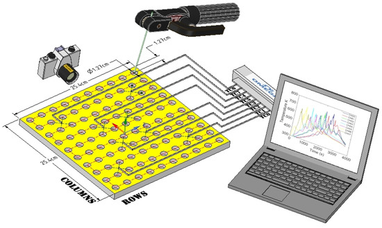
Figure 1.
Plate arrangement with blind holes, thermocouple distribution, and data acquisition.
The welding material was deposited into the blind holes, starting at the initial electrode position (see Figure 1). This position was designated as column 1, row 1 (C1, R1). From this point, the process followed the red line marking the trajectory, creating a zigzag pattern across the plate.
The welding procedure was carried out using a UR10 Universal Robot (Universal Robots A/S, Odense, Denmark) programmed with the precise coordinates of the 100 welding points. This configuration allowed precise control over welding duration and electrode positioning. Each hole was welded for 15 s, followed by a 15 s rest. The total welding process lasted 3000 s, and material deposition began 50 s after the data acquisition system was activated. The thermal histories recorded by the thermocouples extended up to 3750 s.
The welding machine operated at a constant current of 240 A, using a 2.4 mm diameter flux-cored wire that deposits a high chrome carbide alloyed weld metal with excellent abrasion and moderate impact resistance.
In addition to localized temperature measurements taken with thermocouples, global thermal analyses were performed using a Fluke Ti-32 thermal imaging camera (Fluke Corporation, Everett, WA, USA), capable of measuring temperatures between 285 and 900 K at various process stages.
2.2. General Transport Equations
This study models the transient heat transfer in a solid plate induced by welding. The analysis is limited to conduction within the plate material, natural convection, and radiation to the surroundings, excluding other transport mechanisms such as mass transfer.
To model heat transfer involving these three mechanisms, Fluent CFD (Ansys, Inc., Canonsburg, PA, USA, Version 2023 R1) a computational fluid dynamics software was employed to numerically solve the general energy equation (Equation (1)):
where E is the total specific energy, is the density, k is the thermal conductivity, T is the temperature, p is the pressure, is the flow velocity, and is the heat source term associated with the welding process.
The relationship for E is given by
where h is the enthalpy. A user-defined function (UDF) is utilized to compute the heat loss at the walls, based on Equation (3):
where is the total heat transfer coefficient, is the convection heat transfer coefficient, and is the radiation heat transfer coefficient.
Heat loss due to free convection is modeled using the coefficients proposed by W. H. McAdams [25] for atmospheric conditions, assuming a hot upper surface and a cold lower surface. To determine the flow regime, the Rayleigh number is calculated as
where is the Grashof number, and is the Prandtl number.
The film temperature is calculated as
where is the wall temperature, and is the ambient temperature.
For laminar flow, when , the convection heat transfer coefficient is given by
For turbulent flow, when , the convection heat transfer coefficient is
The heat loss coefficient due to radiation is calculated using Equation (6). According to [26,27], this coefficient becomes significant when radiation heat transfer is dominant, particularly in high-temperature scenarios. At elevated temperatures, radiation heat transfer becomes the primary heat dissipation mode and must be accounted for to achieve accurate thermal calculations.
where is the Stefan–Boltzmann constant. A macro is employed to calculate the convection and radiation coefficients, which measure the temperature of the faces of each cell in the mesh at the wall.
2.3. Heat Source Model
The heat source used in the welding process was modeled using a user-defined function (UDF), as shown in Figure 2. This function simulates heat generation within a uniform cylindrical volume, similar to the approaches presented in [28,29,30,31]. The cylindrical volume corresponds to the size of the hole, providing an accurate representation of the heat generated and distributed within this virtual volume. This approach enables a realistic heat transfer simulation in this geometry’s welding processes.
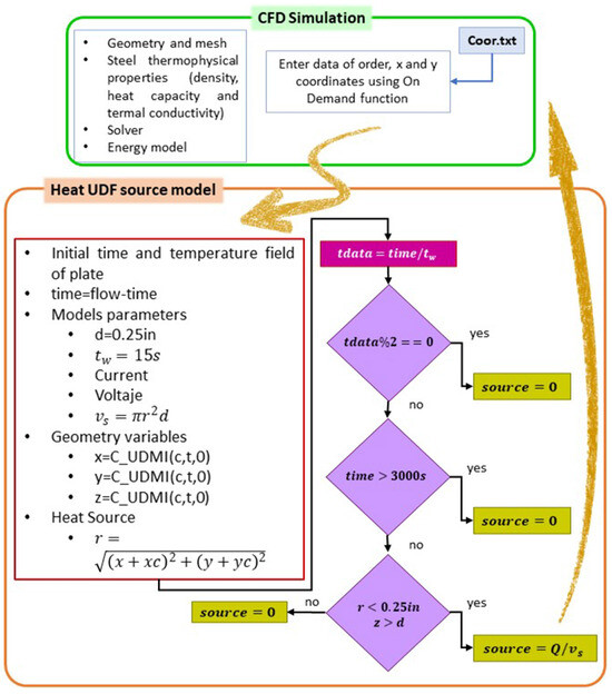
Figure 2.
Heat transfer simulation of the welding process.
The model assumes that the heat generated in the welding zone is uniformly distributed within the cylindrical volume. This approach is particularly suitable for simulating thermal behavior in deep welding processes. The cylindrical model is especially advantageous when volumetric heat sources are required, rather than surface distributions, as discussed in [32]. Equation (7) models the heat generated per unit volume, offering a detailed representation of heat transfer in these processes.
represents the heat generated by the electric arc, calculated using the welding equipment power multiplied by the process thermal efficiency, typically ranging from 70% to 85% as per [33]. For this analysis, an efficiency value of 80% is assumed. , on the other hand, represents the volume of the circular heat source and is expressed as , where r and d are the radius and depth of the blind hole, respectively.
A UDF in C language is employed to model the welding heat source, integrated with the ANSYS CFD software to implement the algorithm shown in Figure 2. This code defines key parameters such as welding, resting, and welding power. The process begins by defining the energy transport equation and a custom function to calculate , the mesh model, and material properties.
The welding position and order, arranged in descending order, are obtained by reading a file containing the coordinates x and y using the On Demand function. The volumetric heat generation term is applied individually at each site, following a sequential order of 100 points defined in the Coor.txt file. For each welding point, 15 s of welding and 15 s of rest are applied, with the condition that the total simulation time is at most 3000 s. The coordinates x and y represent the welding positions and are sorted for implementation.
The volume of the heat source is defined by the domain delimitation, using the information provided by the variables x, y, and z, which describe the mesh geometry.
2.4. FNN Model Design
This section explains the design of the feedforward neural network (FNN) model used to predict the area under the temperature curve in the welding process. It covers the network architecture, selected hyperparameters, and the training process based on data from CFD simulations. The model’s performance relies on key quantitative indicators, including mean squared error (MSE), mean absolute percentage error (MAPE), and the coefficient of determination (). The neural network improves prediction accuracy by adjusting weights through an optimization process that minimizes error. This section also details the hyperparameters used to configure the FNN and the criteria used to assess model performance.
In general, the architecture used in this work consists of an FNN with an input layer of 100 neurons, corresponding to the values of the 100 coordinates representing the positions of the welding trajectory. The network has three hidden layers: the first with 256 neurons, the second with 128 neurons, and the third with 64 neurons. The output layer has a single neuron that predicts the area calculated under the temperature curve. The hyperparameters used in the model implementation are as follows:
- Activation function: ReLU (Rectified Linear Unit) in all hidden layers. Expressed as
- Identity activation function in the output layer, represented as
- The model trains using the Adam optimizer (Adaptive Moment Estimation), which combines momentum optimization and RMSProp (Root Mean Square Propagation), making it suitable for deep neural networks. The mathematical equations involved with the Adam optimizer arewhere and are the decay factors of the moments (typically and ), and is the gradient of the loss function concerning the parameters.Next, the parameters correct the bias of the moments and using the following corrections:Finally, update the parameters using the following rule:where is the learning rate, and is a small constant value (typically ) to avoid division by zero.This work used this method to adjust the model weights during training with a learning rate of and momentum parameters (, ).
- L2 regularization (with a value of 0.001) was applied to prevent overfitting.
- The Dropout (0.2) indicates that, during training, 20% of the neurons will be randomly deactivated at each step, which helps the model to better generalize.
- Early stopping with patience set to 10 epochs was used to halt training when validation loss stopped improving.
- Number of training epochs: 200.
- Percentage of data for training: 80%, with the remaining 20% used for validation and testing.
The model trains using data generated by CFD simulations. During training, the model adjusts the neurons’ weights to minimize the mean squared error (MSE) between the network’s predictions and the actual values obtained from the simulations. The data generation process with the CFD simulation runs in parallel, taking advantage of multiple CPU cores to reduce computation time. When the CFD data generation is completed, the trapezoidal rule calculates the area under the temperature curves, ensuring an accurate estimation of the integral of the temperature curve over time.
Early Stopping is a regularization technique used to prevent overfitting during training. It promotes the model’s generalization to new, unseen data. Early Stopping was used to monitor the validation loss with a patience value of 20 epochs.
The quality criteria adopted to evaluate the trained FNNs include three key quantitative metrics: the mean absolute percentage error (MAPE), the mean squared error (MSE), and the coefficient of determination (). These are detailed below:
- 1.
- Mean absolute percentage error (MAPE) measures the model’s accuracy in relative terms, showing the average difference between predicted and actual values as a percentage.where is the actual value, is the predicted value, and n is the total number of data points.
- 2.
- Mean squared error(MSE) is another metric used to evaluate the difference between predicted and actual values, penalizing larger errors more significantly, and allowing assessment of the global fit of the model.where is the actual value, is the predicted value, and n is the total number of data points.
- 3.
- R-squared () evaluates the degree of fit of the model, indicating the proportion of variance in the data explained by the model. A value of close to 1 suggests that the model explains the data well.where is the actual value, is the predicted value, is the mean of the actual values, and n is the total number of data points.
Using these three metrics allowed a comprehensive evaluation of the model’s performance.
Table 1 presents a comparative analysis of the performance of different neural network architectures with one, two, and three hidden layers, varying the number of neurons in each layer. The metrics MSE, , and MAPE analyze the training and validation sets.

Table 1.
Metrics of different neural network architectures.
The models with a single hidden layer showed relatively high values of MSE and MAPE, as well as lower coefficients in validation, indicating lower generalization capacity. On the other hand, networks with three hidden layers achieved the best results, particularly the 256–128–64 configuration, with the lowest MSE in validation (0.0186) and the highest (0.8430), suggesting greater accuracy and stability in predictions. The training MAPE (3.6280%) and validation MAPE (4.2830%) values indicate no overfitting.
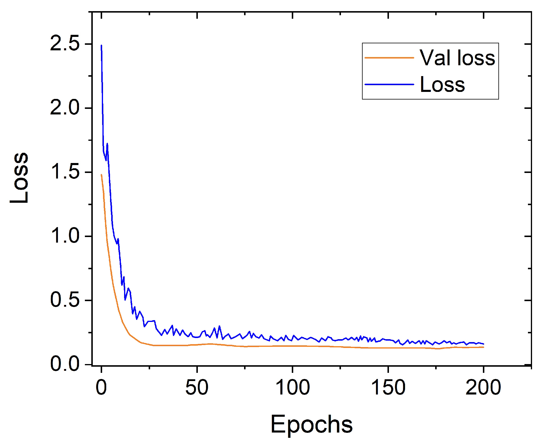
Figure 3 shows the evolution of the loss function (Loss) and validation loss (Val Loss) across the epochs. Both curves decrease quickly at the beginning and stabilize as the training progresses.
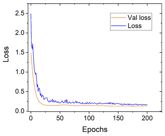
Figure 3.
Evolution of the loss during training (corregir val por val loss).
Early Stopping indicated that, in all cases, training stopped near 200 epochs, which represents optimal convergence for the model. Stopping at 200 epochs prevents overfitting and ensures the model generalizes well.
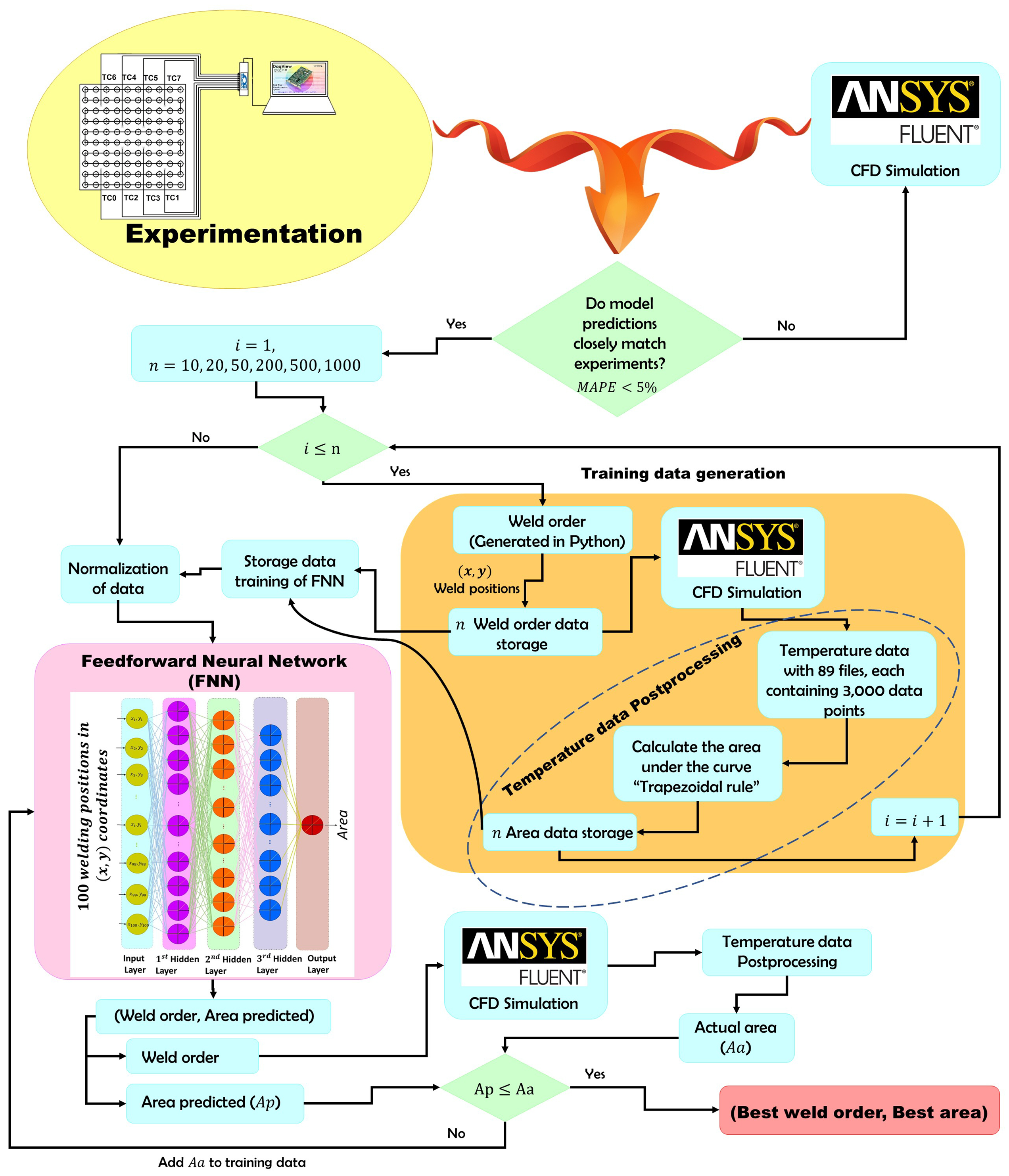
2.5. Hybrid Model CFD-FNN
The hybrid model in Figure 4 executes a series of computational simulations to optimize heat transfer during welding, leveraging computational fluid dynamics (CFD) simulations and neural networks.
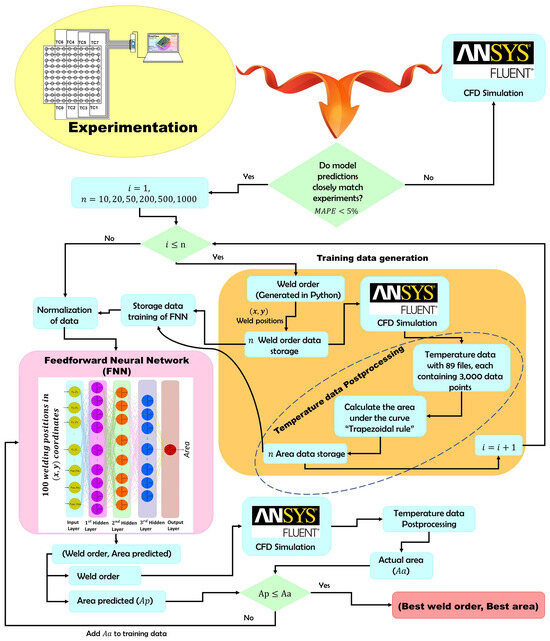
Figure 4.
Hybrid model CFD-FNN used to optimize heat transfer during welding.
The objective function was to minimize the area under the temperature history curves at multiple welding sites, enhancing thermal management and preventing overheating.
The hybrid model begins by generating random welding order coordinates for the welding application at different sites. It then uses these sequences to make a CFD welding process simulation to obtain temperature evolution data for 89 sites.
A welding sequence is generated for n simulations, and a PowerShell script runs each Fluent CFD simulation in different directories in parallel to accelerate the modeling process. The script retrieves temperature data from multiple output files generated during the simulation and calculates the area under the curve using a numerical integration method. It takes the maximum temperature at each time across all curves and applies the trapezoidal rule. These n areas are used for training the network.
Next, the training data are normalized to ensure that all input values are on a similar scale, improving the neural network’s performance and convergence speed. Then, a deep FNN model trains using Keras, specifically through the Sequential class, to predict the area under the curve for new sequences. The model uses 80% of the data for training and 20% for validation and testing. The training data consist of welding orders and their corresponding areas generated from multiple CFD simulations. The model follows a sequential architecture with fully connected layers, featuring 100 inputs corresponding to the 100 values of the welding application order. It has three hidden layers: the first with 256 neurons, the second with 128 neurons, and the third with 64 neurons.
The network produces a single output, predicting the area calculated as a regression task. ReLU functions in each hidden network layer, while the output layer requires an identity activation function. The learning procedure starts at the input layer, propagating the training data through the network to generate an output. The system calculates the mean squared error (between the predicted and calculated areas) from the output, and the Adam optimizer minimizes this error. Forward propagation computes the output after repeating the procedure for 200 epochs and learning the weights.
After training, the model proposes a new welding order and calculates the predicted area. The system compares the predicted area with the actual area calculated from an additional CFD simulation. If the predicted area is less than or equal to the actual area, it is considered the best-performing welding order. Otherwise, the system feeds the actual area into the network and validates it with a new simulation.
2.6. Consideration of the Model
The simulation model incorporates the geometric dimensions of the welding plate to ensure dimensional accuracy between the experiment and the simulation. The boundary conditions account for heat dissipation through natural convection with air and heat transfer by radiation to the surrounding environment across all domain walls. The initial temperature for both the plate and the surrounding medium equals 283.15 K.
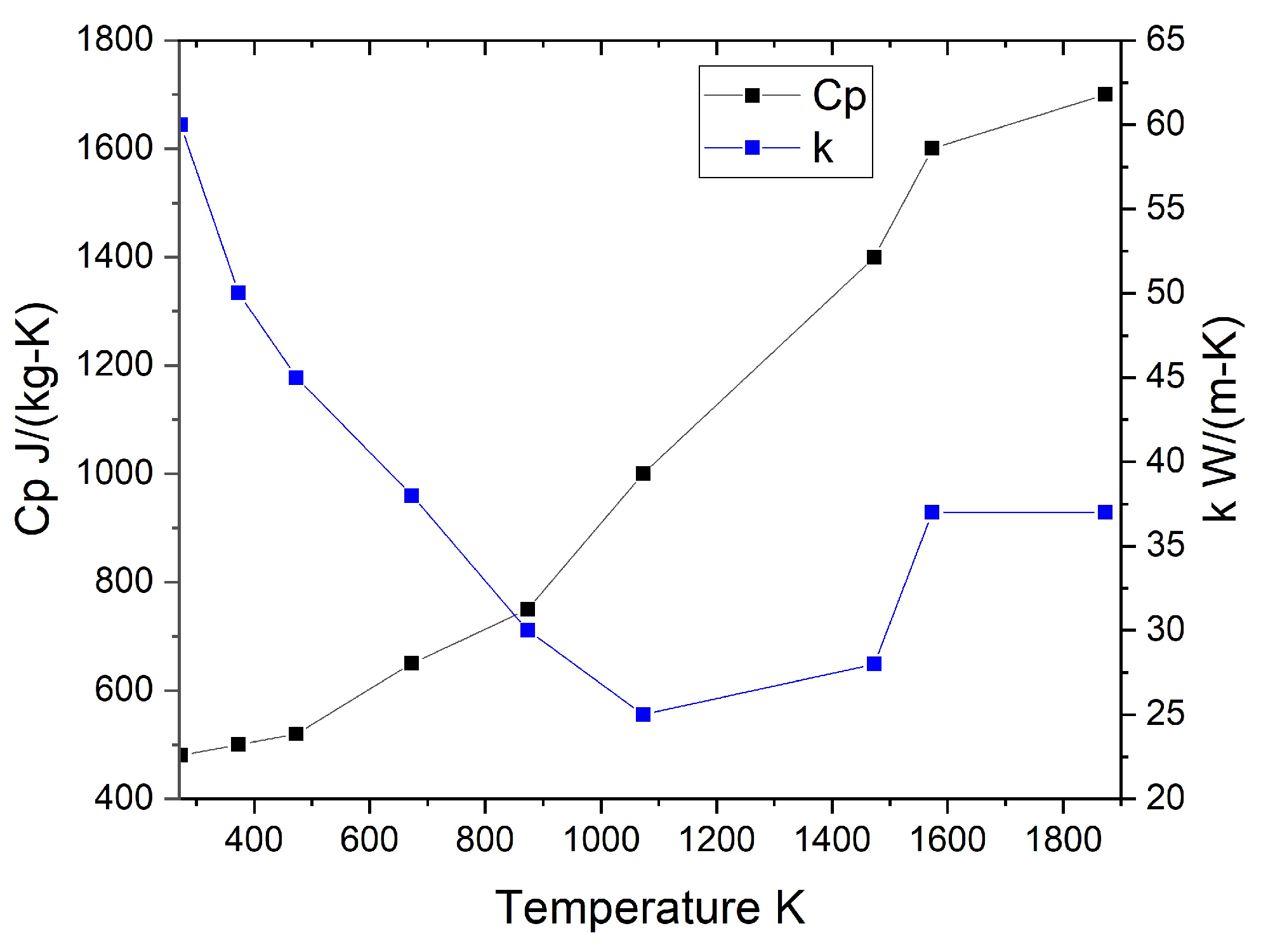
Thermophysical properties, such as specific heat and thermal conductivity of AISI 1018 carbon steel, come from the works of Jeyakumar et al. [34] and Nadimi et al. [35]; see Figure 5. Density is set to a constant value of 7850 , and an emissivity of 0.8 is applied, as recommended by De et al. [36].
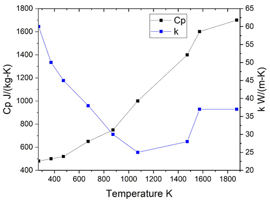
Figure 5.
Temperature-dependent properties of AISI 1018 carbon steel.
The modeled computational domain excludes the drilled blind holes and considers a simplified flat plate geometry. The mesh used for discretizing the domain contains 25,000 cells, providing sufficient resolution to capture the plate’s thermal behavior during the welding process. The energy equation is solved with second-order upwind spatial discretization, applying an absolute convergence criterion of 1e-6 and a time step of 0.01 s.
In the simulation, thermocouples placed between each blind hole covered 89 sites, generating 89 files that stored the temporal evolution of the temperature. These files were used to calculate the area under the curve, constructed by using the highest temperature value at each time step. The number of simulations considered were 10, 20, 50, 200, 500, and 1000. This approach enabled the observation of improvements in the thermal management of the welding process, providing a detailed analysis of heat distribution and evolution based on the number of simulations, ultimately contributing to process optimization.
Two workstations ran the hybrid model: one with a 16-core 3.2 GHz CPU and 64 GB of RAM and another with a 20-core 2.4 GHz CPU and 32 GB of RAM. Once the neural network was validated, the calculations and simulations took approximately 78 days to complete.
3. Experimental and Numerical Results
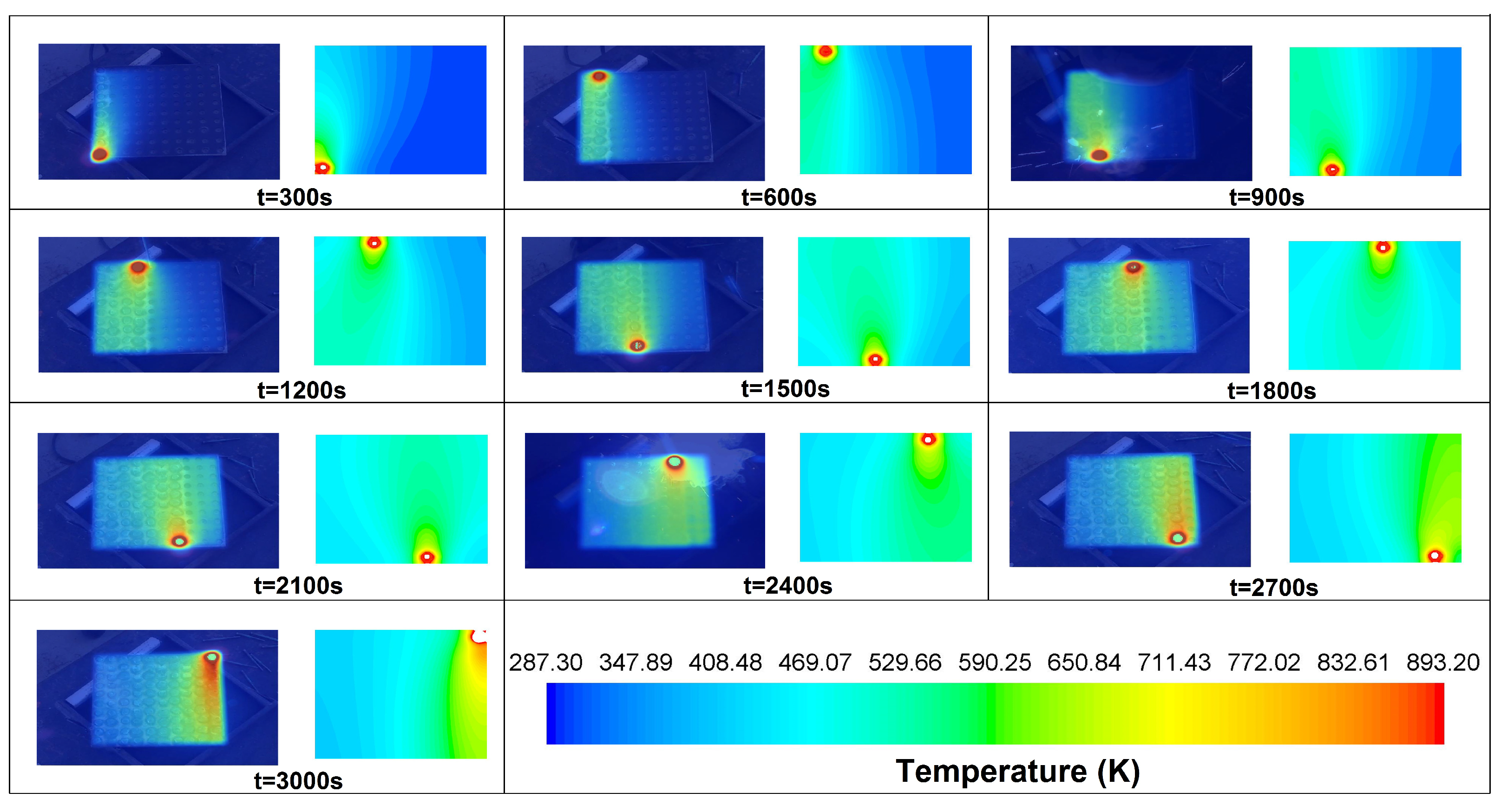
Figure 6 shows a general comparison of the temperature fields obtained. The images on the left display thermographic measurements taken during the experiments, while the images on the right show results from the simulation, with temperature values adjusted within the measurement range handled by the thermographic camera. The notable similarities between the experimental and simulated results validate the numerical model used in this study. Both methodologies accurately capture the main characteristics of heat propagation during the welding process.
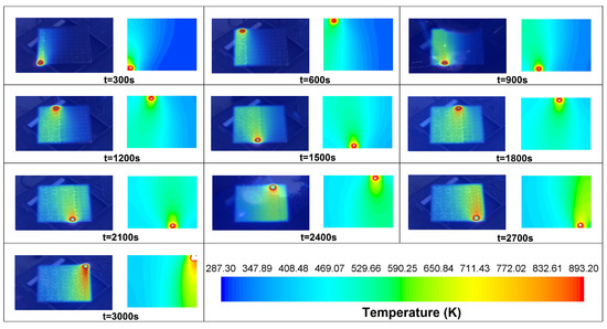
Figure 6.
Comparison of simulation results and thermography at different times.
The agreement in the spatial distribution of heat and the maximum and minimum temperatures demonstrates a good correspondence between the experimental and simulated results. Additionally, the thermal response times between both methods show remarkable consistency, reinforcing the reliability of the numerical model and its ability to predict thermal behavior accurately.
The simulation reproduces the thermal concentration zones and the heat dissipation paths, highlighting the robustness of the numerical approach in predicting thermal evolution. However, slight deviations appear in areas with high temperatures. Several factors may explain these differences, including simplifications of the physical model, numerical averaging, and the inherent dissipation in the algorithms, which may smooth finer details found in the experimental data [37].
Additionally, the absence of experimental noise in the simulation results in smoother thermal transitions compared to the thermographic captures. Despite these variations, the model’s overall accuracy remains intact, as thermal trends and the spatial distribution of heat stay consistent in both approaches. This suggests that the numerical simulation effectively predicts thermal behavior in welding processes, providing valuable information for optimization.
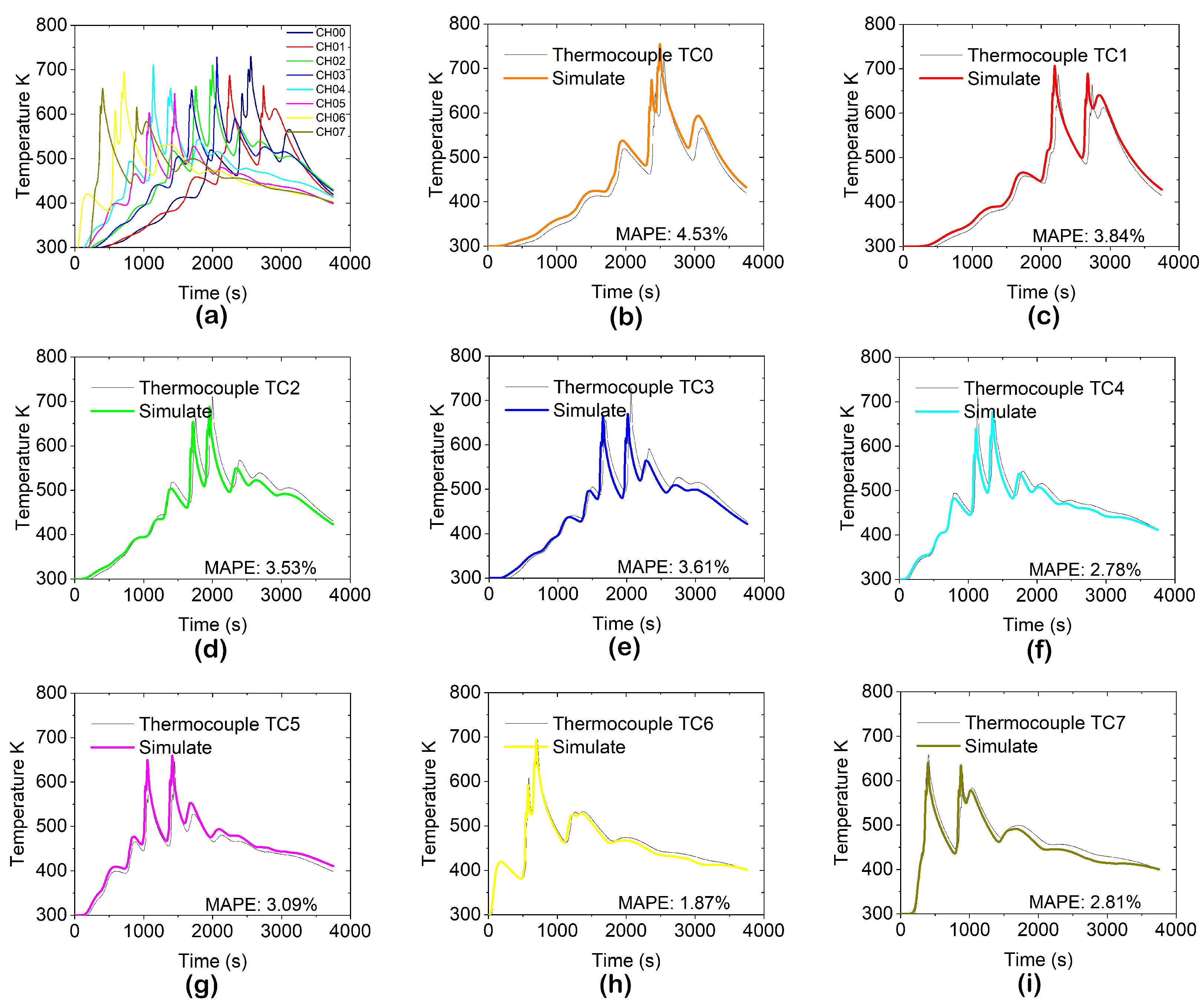
Figure 7 compares the experimental measurements and simulation results for the thermal history at eight different sites of the welding process, measured by the thermocouples TC0 to TC7. The results show significant similarities in the trends and magnitudes of the temperatures. For all thermocouples, the simulation captures the formation of the primary peaks and valleys observed in the experimental data, especially during the heating and cooling phases of the welding process.
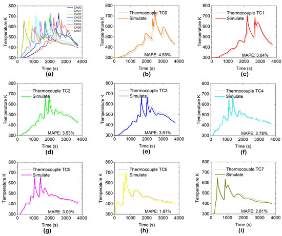
Figure 7.
Temperature evolution at different thermocouple locations. Subfigures (a–i) compare simulated and experimental temperature data for thermocouples TC0–TC7. The mean absolute percentage error (MAPE) quantifies the simulation’s accuracy in predicting thermal behavior.
Although some sites show slight delays or minor differences in peak size, particularly during abrupt temperature changes, factors such as numerical averaging, geometric or temporal discretization, and inherent smoothing in the simulations likely explain these variations. These peaks typically exhibit more pronounced variations in the experimental data, as mentioned in [37].
Despite these differences, the overall trend agreement validates the model’s predictive ability. The observed variations do not affect the model’s performance but emphasize the typical trade-offs in computational simulations, such as simplified physics and numerical dissipation, which tend to smooth sharp and localized temperature changes. Furthermore, the calculation of the MAPE errors for each monitor ranges from 1.87% to 4.53% (see Figure 7).
Real-world sensors capture these changes more accurately but may need to be more evident in the simulations. However, both datasets are recorded at the same frequency, with one data point per second.
Ultimately, the overall agreement between the two methods demonstrates the simulation’s strength in replicating experimental conditions. This result becomes especially significant when considering the limitations and approximations inherent in numerical modeling and the experimental setup.
After selecting the optimal neural network architecture with a structure of 256–128–64 neurons in its respective hidden layers, various tests were conducted by varying the training set size. These experiments aimed to evaluate the model’s performance in terms of mean squared error (MSE), coefficient of determination (), and mean absolute percentage error (MAPE) in both the training and validation phases.
Table 2 shows the validation results for different training set sizes. The MSE decreases in training and validation phases as the training size increases, indicating higher prediction accuracy. Similarly, the coefficient improves, suggesting a better ability to explain data variability. Moreover, the MAPE tends to decrease, reflecting a more precise relative prediction error. However, while improvements continue as dataset size increases, the additional benefits become less significant beyond . Although the model performs best with 1000 training points, the additional gains in validation metrics are marginal considering the time and computational cost of the additional simulations. A training size between 200 and 500 data points offers an optimal trade-off between predictive accuracy and computational efficiency.
Table 2.
Metrics of neural network models with different training set sizes (MSE, , and MAPE).
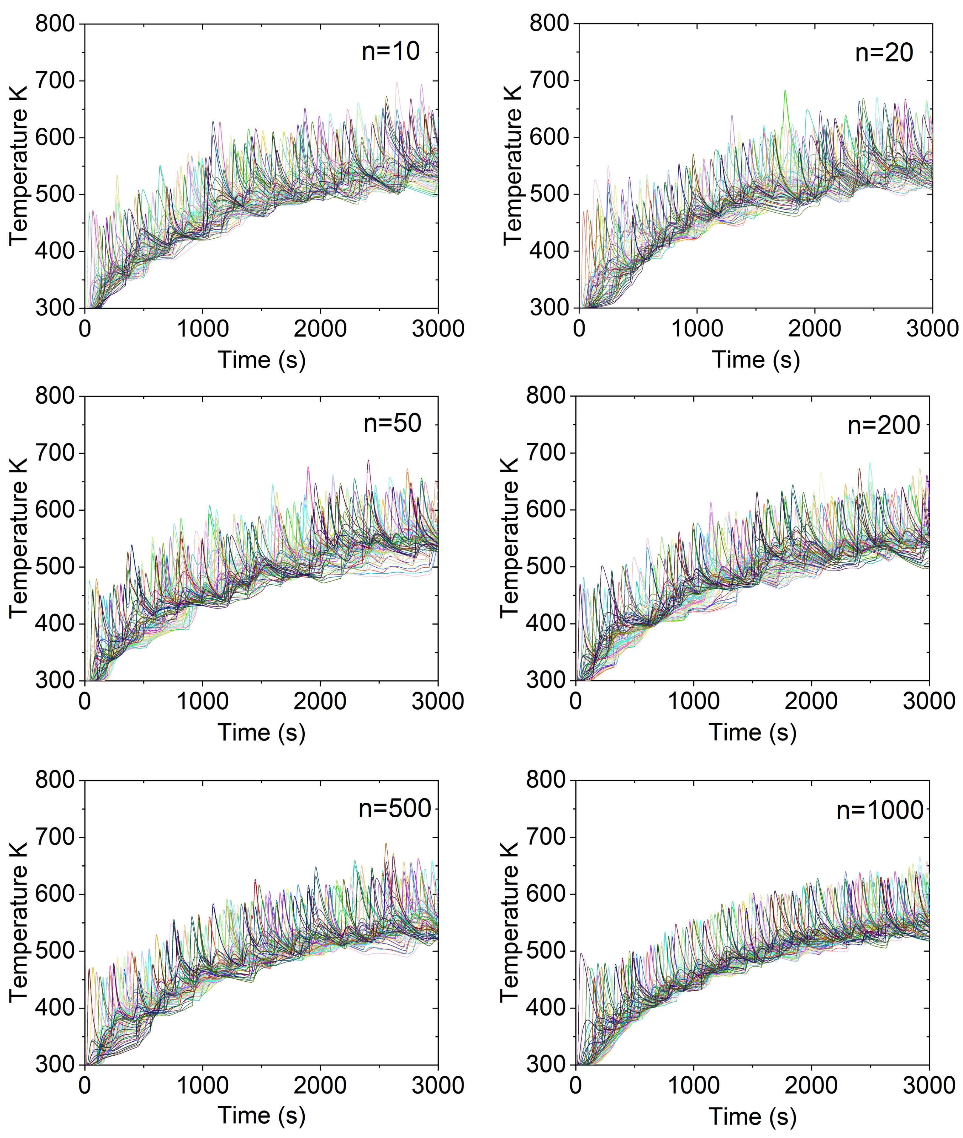
Figure 8 compares the thermal management results of training a neural network with different numbers of training data in the optimization process. The figure illustrates the temperature evolution during welding for n dataset sizes: 10, 20, 50, 200, 500, and 1000 simulations. The training dataset used the area under the curve generated by each simulation. As the number of data increases, the neural network model becomes more accurate in optimizing thermal distribution.
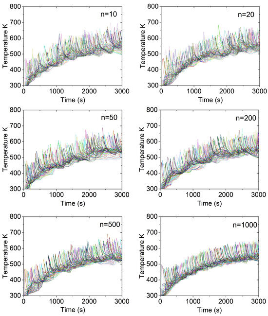
Figure 8.
Comparison of thermal management for neural network training with different dataset sizes.
The temperature curves show more scattering and higher variability in cases with fewer data points ( and ). This suggests that the model needs help to capture the complex heat transfer dynamics, resulting in suboptimal optimization outcomes. With a limited number of training data, the neural network cannot properly learn the thermal patterns of the welding process, which leads to steeper thermal gradients and a higher likelihood of overheating or thermal concentration.
As the training dataset size increases ( 50, 200, 500, 1000), the neural network progressively refines its ability to optimize the thermal coupling between welding points. This results in more uniform thermal gradients and improved heat distribution control. Larger datasets allow the model to learn more complex patterns in the thermal distribution, leading to smoother temperature variations and reduced excessive heat accumulation. Notably, cases with and 1000 show significant improvements in temperature control, suggesting that even larger datasets further enhance model performance.
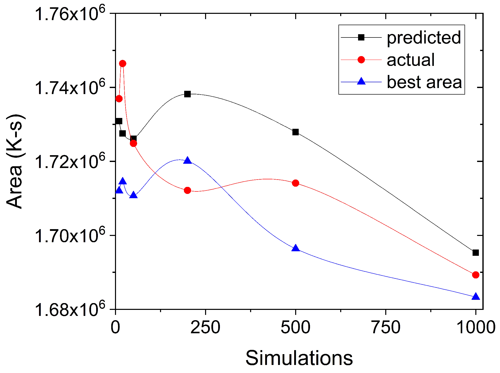
Figure 9 shows the evolution of the three types of area (the predicted area from the neural network, the actual area in the CFD model, and the optimal or best area) as the number of simulations increases.
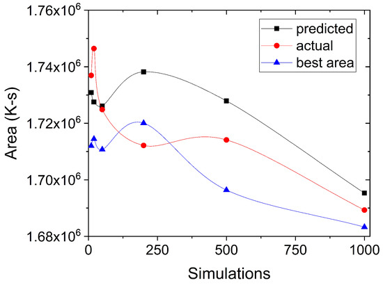
Figure 9.
Training dataset.
As the simulation size increases, the three areas decrease, suggesting a progressive improvement in the model’s ability to optimize the thermal distribution.
In particular, the Best Area curve shows how the neural network finds more optimal solutions as it receives more data, reflecting a convergence towards better thermal management. The differences between the predicted and actual areas at the beginning indicate the need for a larger dataset to improve the model’s accuracy.
As the simulation increases, the model stabilizes, progressively bringing the prediction closer to the actual area. This demonstrates the neural network’s effectiveness in optimizing the thermal distribution of the welding process.
4. Conclusions
Combining CFD simulations with deep neural networks offers an innovative and practical approach to solving complex thermal management challenges in industrial welding processes. This study introduces a hybrid model that integrates computational fluid dynamics simulations with deep neural networks to optimize welding processes.
The comparison between experimental and simulated data revealed good agreement, confirming the CFD model’s accuracy and highlighting its potential for future research in thermal management. The CFD simulation model maintained high stability and accuracy, achieving a mean absolute percentage error (MAPE) below 4.53% when comparing experimental and CFD simulation data.
The hybrid CFD-FNN model achieved a determination coefficient () of up to 0.93 in validation datasets and an MAPE of 3.5%, demonstrating its ability to predict areas under thermal curves in multisite welding processes.
The thermal optimization with neural networks trained with over 500 data points generated trajectories, which reduced thermal variability and improved heat distribution uniformity compared to initial trajectories. This approach lowered peak temperatures, minimized overheating, and ensured a more uniform thermal energy distribution, which could help prevent structural damage to the base material. The results show significant improvements, such as reducing thermal gradients and minimizing the affected thermal zone. The improved temperature field presumably reduces the zone of the detrimental thermal effects such as deformations, stresses, and microstructure; however, more research is needed to quantify them.
The hybrid model predicts the welding process thermal evolution at a reasonable computational cost and suggests an optimal execution sequence to reduce thermal gradients. The presented methodology allows adaptation (with the respective modifications) to other industrial processes involving multipoint welding, welding beads, or additive manufacturing, significantly expanding its applicability in scenarios that require precise thermal management.
Author Contributions
Conceptualization, A.R.M.-G. and S.A.A.-V.; methodology, A.R.M.-G. and S.A.A.-V.; software, A.R.M.-G. and S.A.A.-V.; validation, A.P.-A., A.R.M.-G. and S.A.A.-V.; formal analysis, A.R.M.-G. and S.A.A.-V.; investigation, I.C.-R., A.P.-A. A.R.M.-G., and S.A.A.-V.; resources, R.S.-C. and H.J.V.-H.; data curation, A.R.M.-G. and S.A.A.-V.; writing—original draft preparation, A.R.M.-G. and S.A.A.-V.; writing—review and editing, I.C.-R., A.P.-A., A.R.M.-G. and S.A.A.-V.; visualization, I.C.-R., A.P.-A., A.R.M.-G. and S.A.A.-V.; supervision, R.S.-C. and H.J.V.-H.; project administration, R.S.-C. and H.J.V.-H. All authors have read and agreed to the published version of the manuscript.
Funding
This research received no external funding.
Data Availability Statement
The original contributions presented in this study are included in the article material. Further inquiries can be directed to the corresponding author.
Acknowledgments
The authors thank Dirección de Investigación y Posgrado from UAdeC for their continuous support of the Mechanical Engineering Department. The authors thank the National Laboratory SEDEAM-CONAHCYT. The authors thank CONAHCYT and PRODEP for their continuous support to the Mechanical Engineering Department.
Conflicts of Interest
The authors declare no conflicts of interest.
References
- De Soldadura, M. Recuperacion de un Molino Vertical Atox 32.5 para Molienda de Caliza. Sci. Tech. 2007, 13, 625–630. [Google Scholar]
- Goldak, J.; Bibby, M.; Moore, J.; House, R.; Patel, B. Computer modeling of heat flow in welds. Metall. Trans. 1986, 17, 587–600. [Google Scholar] [CrossRef]
- Cohal, V. Some considerations regarding the thermal field at welded joints. In Proceedings of the IOP Conference Series: Materials Science and Engineering; IOP Publishing: Bristol, UK, 2018; Volume 400, p. 042011. [Google Scholar]
- Brust, F.; Kim, D. Mitigating welding residual stress and distortion. In Processes and Mechanisms of Welding Residual Stress and Distortion; Elsevier: Amsterdam, The Netherlands, 2005; pp. 264–294. [Google Scholar]
- Wu, C.; Wang, C.; Kim, J.W. Welding sequence optimization to reduce welding distortion based on coupled artificial neural network and swarm intelligence algorithm. Eng. Appl. Artif. Intell. 2022, 114, 105142. [Google Scholar] [CrossRef]
- Girón-Cruz, J.A.; Pinto-Lopera, J.E.; Alfaro, S.C. Weld bead geometry real-time control in gas metal arc welding processes using intelligent systems. Int. J. Adv. Manuf. Technol. 2022, 123, 3871–3884. [Google Scholar] [CrossRef]
- Zhang, Y.; Wang, Q.; Liu, Y. Adaptive intelligent welding manufacturing. Weld. J. 2021, 100, 63–83. [Google Scholar] [CrossRef]
- Aguado, A.; Gómez, A.; del Pozo, A. Controlador predictivo neuro-genético. Rev. Iberoam. Autom. Inform. Ind. RIAI 2007, 4, 94–108. [Google Scholar] [CrossRef]
- Waheed, R.; Saeed, H.; Butt, S.; Anjum, B. Framework for Mitigation of Welding Induced Distortion through Response Surface Method and Reinforcement Learning. Coatings 2021, 11, 1227. [Google Scholar] [CrossRef]
- Yang, H.; Shao, H. Distortion-oriented welding path optimization based on elastic net method and genetic algorithm. J. Mater. Process. Technol. 2009, 209, 4407–4412. [Google Scholar] [CrossRef]
- Zhang, H.; Li, R.; Yang, S.; Liu, Z.; Xiong, M.; Wang, B.; Zhang, J. Experimental and Simulation Study on Welding Characteristics and Parameters of Gas Metal Arc Welding for Q345qD Thick-Plate Steel. Materials 2023, 16, 5944. [Google Scholar] [CrossRef]
- Arora, H.; Singh, R.; Brar, G.S. Thermal and structural modelling of arc welding processes: A literature review. Meas. Control. 2019, 52, 955–969. [Google Scholar] [CrossRef]
- Mohanty, U.K.; Sharma, A.; Abe, Y.; Fujimoto, T.; Nakatani, M.; Kitagawa, A.; Tanaka, M.; Suga, T. Thermal modelling of alternating current square waveform arc welding. Case Stud. Therm. Eng. 2021, 25, 100885. [Google Scholar] [CrossRef]
- Mohan, A.; Ceglarek, D.; Auinger, M. Numerical modelling of thermal quantities for improving remote laser welding process capability space with consideration to beam oscillation. Int. J. Adv. Manuf. Technol. 2022, 123, 761–782. [Google Scholar] [CrossRef]
- Chen, F.F.; Xiang, J.; Thomas, D.G.; Murphy, A.B. Model-based parameter optimization for arc welding process simulation. Appl. Math. Model. 2020, 81, 386–400. [Google Scholar] [CrossRef]
- Eagar, T.; Tsai, N. Temperature fields produced by traveling distributed heat sources. Weld. J. 1983, 62, 346–355. [Google Scholar]
- Goldak, J.; Chakravarti, A.; Bibby, M. A new finite element model for welding heat sources. Metall. Trans. B 1984, 15, 299–305. [Google Scholar] [CrossRef]
- Van Elsen, M.; Baelmans, M.; Mercelis, P.; Kruth, J.P. Solutions for modelling moving heat sources in a semi-infinite medium and applications to laser material processing. Int. J. Heat Mass Transf. 2007, 50, 4872–4882. [Google Scholar] [CrossRef]
- Zhou, Z.; Shen, H.; Liu, B.; Du, W.; Jin, J. Thermal field prediction for welding paths in multi-layer gas metal arc welding-based additive manufacturing: A machine learning approach. J. Manuf. Process. 2021, 64, 960–971. [Google Scholar] [CrossRef]
- Ren, K.; Chew, Y.; Zhang, Y.; Bi, G.; Fuh, J. Thermal analyses for optimal scanning pattern evaluation in laser aided additive manufacturing. J. Mater. Process. Technol. 2019, 271, 178–188. [Google Scholar] [CrossRef]
- Mughal, M.; Fawad, H.; Mufti, R. Finite element prediction of thermal stresses and deformations in layered manufacturing of metallic parts. Acta Mech. 2006, 183, 61–79. [Google Scholar] [CrossRef]
- Kasilingam, S.; Yang, R.; Singh, S.K.; Farahani, M.A.; Rai, R.; Wuest, T. Physics-based and data-driven hybrid modeling in manufacturing: A review. Prod. Manuf. Res. 2024, 12, 2305358. [Google Scholar] [CrossRef]
- Romero-Hdz, J.; Aranda, S.; Toledo-Ramirez, G.; Segura, J.; Saha, B. An Elitism Based Genetic Algorithm for Welding Sequence Optimization to Reduce Deformation. Res. Comput. Sci. 2016, 121, 17–36. [Google Scholar] [CrossRef]
- Yuan, M.; Liu, S.; Gao, Y.; Sun, H.; Liu, C.; Shen, Y. Immune Optimization of Welding Sequence for Arc Weld Seams in Ship Medium-Small Assemblies. Coatings 2022, 12, 703. [Google Scholar] [CrossRef]
- McAdams, W.H. Heat Transmission; McGraw-Hill Book Company: New York, NY, USA, 1954. [Google Scholar]
- López-Cornejo, M.S.; Vergara-Hernández, H.J.; Arreola-Villa, S.A.; Vázquez-Gómez, O.; Herrejón-Escutia, M. Numerical Simulation of Wire Rod Cooling in Eutectoid Steel under Forced-Convection. Metals 2021, 11, 224. [Google Scholar] [CrossRef]
- López-Martínez, E.; Hernández-Morales, J.; Solorio-Díaz, G.; Vergara-Hernández, H.; Vázquez-Gómez, O.; Garnica-González, P. Predicción del perfil de dureza en probetas jominy de aceros de medio y bajo carbono. Rev. Mex. Ing. Quím. 2013, 12, 609–619. [Google Scholar]
- Jia, L.; Zou, Y.; Zou, Z.D.; Zhao, Y.S.; Yao, Q.S. Research and application status of arc welding heat source model for T-joint numerical simulation. Adv. Mater. Res. 2011, 154, 1423–1426. [Google Scholar] [CrossRef]
- Belhadj, A.; Bessrour, J.; Masse, J.E.; Bouhafs, M.; Barrallier, L. Finite element simulation of magnesium alloys laser beam welding. J. Mater. Process. Technol. 2010, 210, 1131–1137. [Google Scholar] [CrossRef]
- Doshi, S.; Jani, D.; Gohil, A.; Patel, C. Investigations of heat source models in transient thermal simulation of pulsed MIG welding of AA6061-T6 thin sheet. In Proceedings of the IOP Conference Series: Materials Science and Engineering; IOP Publishing: Bristol, UK, 2021; Volume 1146, p. 012015. [Google Scholar]
- Kim, C.H.; Zhang, W.; DebRoy, T. Modeling of temperature field and solidified surface profile during gas–metal arc fillet welding. J. Appl. Phys. 2003, 94, 2667–2679. [Google Scholar] [CrossRef]
- Nascimento, E.J.; dos Santos Magalhães, E.; dos Santos Paes, L.E. A literature review in heat source thermal modeling applied to welding and similar processes. Int. J. Adv. Manuf. Technol. 2023, 126, 2917–2957. [Google Scholar] [CrossRef]
- Goldak, J.A.; Akhlaghi, M. Computational Welding Mechanics; Springer Science & Business Media: Cham, Switzerland, 2005. [Google Scholar]
- Jeyakumar, M.; Christopher, T. Influence of residual stresses on failure pressure of cylindrical pressure vessels. Chin. J. Aeronaut. 2013, 26, 1415–1421. [Google Scholar] [CrossRef]
- Nadimi, S.; Khoushehmehr, R.; Rohani, B.; Mostafapour, A. Investigation and analysis of weld induced residual stresses in two dissimilar pipes by finite element modeling. J. Appl. Sci. 2008, 8, 1014–1020. [Google Scholar] [CrossRef]
- de Freitas Teixeira, P.R.; de Araújo, D.B.; da Cunha, L.A.B. Study of the Gaussian distribution heat source model applied to numerical thermal simulations of tig welding processes. Cienc. Eng. Sci. Eng. J. 2014, 23, 115–122. [Google Scholar]
- Oberkampf, W.L.; Roy, C.J. Verification and Validation in Scientific Computing; Cambridge University Press: Cambridge, UK, 2010. [Google Scholar]


Disclaimer/Publisher’s Note: The statements, opinions and data contained in all publications are solely those of the individual author(s) and contributor(s) and not of MDPI and/or the editor(s). MDPI and/or the editor(s) disclaim responsibility for any injury to people or property resulting from any ideas, methods, instructions or products referred to in the content. |
© 2025 by the authors. Licensee MDPI, Basel, Switzerland. This article is an open access article distributed under the terms and conditions of the Creative Commons Attribution (CC BY) license (https://creativecommons.org/licenses/by/4.0/).